A fully coupled Mediterranean regional climate system model: design and evaluation of the ocean component for the 1980–2012 period

Abstract

A fully coupled regional climate system model (CNRM-RCSM4) dedicated to the Mediterranean region is described and evaluated using a multidecadal hindcast simulation (1980–2012) driven by global atmosphere and ocean reanalysis. CNRM-RCSM4 includes the regional representation of the atmosphere (ALADIN-Climate model), land surface (ISBA model), rivers (TRIP model) and the ocean (NEMOMED8 model), with a daily coupling by the OASIS coupler. This model aims to reproduce the regional climate system with as few constraints as possible: there is no surface salinity, temperature relaxation, or flux correction; the Black Sea budget is parameterised and river runoffs (except for the Nile) are fully coupled. The atmospheric component of CNRM-RCSM4 is evaluated in a companion paper; here, we focus on the air–sea fluxes, river discharges, surface ocean characteristics, deep water formation phenomena and the Mediterranean thermohaline circulation. Long-term stability, mean seasonal cycle, interannual variability and decadal trends are evaluated using basin-scale climatologies and in-situ measurements when available. We demonstrate that the simulation shows overall good behaviour in agreement with state-of-the-art Mediterranean RCSMs. An overestimation of the shortwave radiation and latent heat loss as well as a cold Sea Surface Temperature (SST) bias and a slight trend in the bottom layers are the primary current deficiencies. Further, CNRM-RCSM4 shows high skill in reproducing the interannual to decadal variability for air–sea fluxes, river runoffs, sea surface temperature and salinity as well as open-sea deep convection, including a realistic simulation of the Eastern Mediterranean Transient. We conclude that CNRM-RCSM4 is a mature modelling tool allowing the climate variability of the Mediterranean regional climate system to be studied and understood. It is used in hindcast and scenario modes in the HyMeX and Med-CORDEX programs.

• Mediterranean Sea
• regional climate system model
• air-sea fluxes
• hindcast simulation
• interannual variability

1. Introduction

The Mediterranean region is a perfect case study for climate regionalisation. The local climate is defined by a complex topography channelling regional winds (Mistral, Tramontane, Bora, Meltem, Sirocco), many small islands limit the low-level air flow and the coastline is particularly complex. Additional regional characteristics including a strong land–sea contrast, land–atmosphere feedback, intense air–sea coupling and aerosol–radiation interactions must also be taken into account when dealing with Mediterranean climate modelling. Like the Mediterranean climate, the Mediterranean Sea shows a complex bathymetry including narrow and shallow straits, coastal currents, strong eddy activity and various distinct and interacting water masses involved in a deep thermohaline circulation. Rivers also play a key role in the hydrological cycle.

For these reasons, the Mediterranean area is often chosen to test new regional climate modelling tools called regional climate system models (RCSMs), which include a high-resolution and fully coupled representation of most of the physical components of the regional climate system: atmosphere, land surface, vegetation, hydrology, rivers and ocean. These RCSMs belong to the same family as the global earth system models (ESM) used in the CMIP5 experiment. Note that RCSMs have also been developed in other semi-enclosed seas such as the Baltic Sea and the Arctic Sea. For the Mediterranean area, this modelling effort started with daily coupled Atmosphere–Ocean Regional Climate Models (AORCMs) with typical horizontal resolutions of 30–50 km in the atmosphere and 10–20 km in the ocean (Somot et al., 2008; Artale et al., 2010; Herrmann et al., 2011; Krzic et al., 2011; Drobinski et al., 2012; L'Hévéder et al., 2013). More recently, river coupling was added in order to attain the status of RCSMs (Dell'Aquila et al., 2012). Other Mediterranean modelling groups are currently preparing the addition of interactive lakes, vegetation, city, ocean biogeochemistry and aerosols.

The coordination of the Mediterranean regional climate system modelling community started within the European project CIRCE (Gualdi et al., 2013a), through which five AORCMs or RCSMs were intercompared (Dubois et al., 2012; Gualdi et al., 2013b). Nowadays, 11 modelling centres including groups from Italy (ENEA, CMCC), Spain (UCLM/UPM, UAH), France (CNRM, LMD, IPSL), Germany (MPI, GUF), Tunisia (INSTM) and Serbia (Univ. of Belgrade) are coordinated through the Med-CORDEX initiative (Ruti et al., 2014; www.medcordex.eu). Med-CORDEX is both the regional climate modelling taskforce of the HyMeX program (www.hymex.org) and the Mediterranean domain of the international CORDEX program.

As in previous versions [see Somot et al. (2008) for version 1; Somot et al. (2009) and Dubois et al. (2012) for version 2 and Herrmann et al. (2011) for version 3], CNRM-RCSM4 is based on the ARPEGE-ALADIN atmosphere model, the ISBA land-surface model and the OPA-NEMO ocean model to which we added the TRIP river model. CNRM-RCSM4 is a fully coupled model without any constraint at the interfaces between the different components of the system. Thus, the regional climate system evolves with a large degree of freedom. The main drivers are at its lateral boundary conditions, for which we prescribed global atmosphere and ocean reanalyses – that is to say, our best knowledge of the current global climate. The previous RCSMs, as described in the literature, had more constraints than CNRM-RCSM4. The PROTHEUS system (Artale et al., 2010; Carillo et al., 2012; Dell'Aquila et al., 2012) kept the Levitus climatology in the Atlantic part of the model. This is a weak point in studying the system's sensitivity to the Atlantic Multidecadal Oscillation [AMO, Marullo et al. (2011)], as underlined by Mariotti and Dell'Aquila (2012). Moreover, the Black Sea runoff was corrected to match the monthly climatology presented by Stanev and Peneva (2002). L'Hévéder et al. (2013) and Drobinski et al. (2012) used a climatology in the Atlantic part of the system, and observed river runoffs; as did Krzic et al. (2011), whose ocean domain does not include any Atlantic part.

The goal of this paper is to evaluate and analyse the CNRM-RCSM4 simulation for the ERA-Interim period (1979–2012). From the surface fluxes to the deep ocean, from the daily to the climatic scale, we demonstrate the model's ability to reproduce the key Mediterranean processes [regional winds over the sea, strong air–sea fluxes, ocean deep convection, strait dynamics, decadal variability such as Eastern Mediterranean Transient (EMT) and long-term trends]. We also give an overview of the model's performance in simulating the behaviour of the Mediterranean Sea. In this way, we prepare forthcoming scientific studies of Mediterranean climate variability and encourage intercomparisons with other models – for example, in the Med-CORDEX framework.

First, in Section 2, we describe the individual models used for the coupled system (RCSM4 in the following) as well as the coupling. Then, in Section 3, we present the model's lateral boundary conditions and the experimental set-up. The evaluation is presented in Section 4: we focus on the Mediterranean Sea and its forcings (Atlantic, rivers, air–sea fluxes) and compare the model results to observations and gridded products. The atmospheric component of RCSM4 is evaluated in a companion paper (Nabat et al., 2014b). Long-term stability, mean seasonal cycle, interannual variability and decadal trends are analysed. A comparison with state-of-the-art RCSMs, the current limitations of RCSM4, and the evaluation and understanding of trends will be discussed in Section 5. Conclusions and ideas for future improvements are given in Section 6.

2. Model description

2.1. The atmospheric regional model ALADIN-Climate

The ALADIN-Climate model (Radu et al., 2008; Colin et al., 2010; Herrmann et al., 2011) is a bi-spectral regional climate model (RCM) with a semi-implicit semi-Lagrangian advection scheme. Horizontal diffusion, semi-implicit corrections and horizontal derivatives are computed using a finite family of analytical functions. In the case of ALADIN, a 2-D bi-Fourier decomposition is used (Haugen and Machenhauer, 1993). In contrast to the globe, the domain is not periodic, so a bi-periodisation is achieved in grid-point space by adding a so-called extension zone, used only in Fourier transforms. The non-linear contributions to the equations are performed in grid-point space. In this configuration, ALADIN-Climate includes an 11-point wide bi-periodisation zone in addition to the more classical eight-point relaxation zone using the Davies technique. More details can be found in Radu et al. (2008) and Farda et al. (2010). The main physical parameterisations of ALADIN-Climate version 5 are the convection scheme, a mass-flux scheme with convergence of humidity closure based on Bougeault (1985), the cloud scheme based on the Ricard and Royer (1993) statistical scheme and the large-scale precipitation as described by Smith (1990). The radiative scheme is derived from Morcrette (1989) and from the IFS model of the ECMWF. It includes greenhouse gases (CO₂, CH₄, N₂O and CFC) in addition to water vapour and ozone. The scheme also takes into account five classes of aerosols (sulphate, black carbon, organic carbon, desert dust and sea salt). The climatology used comes from Tegen et al. (1997). The aerosols are not transported, they are used by the radiative scheme to diffuse and absorb shortwave and longwave radiations (LW). Nabat et al. (2013) proposed a new climatology of aerosols which is used in Nabat et al. (2014b), with the same CNRM-RCSM4 model. The planetary boundary layer turbulence physics including the computation of the turbulent air–sea fluxes is based on Louis (1979), and the interpolation of the wind speed from the first layer of the model (about 30 m) to the 10 m height follows Geleyn (1988). In the current study, we use a Lambert conformal projection for the pan-Mediterranean domain at an horizontal resolution of 50 km centred at 14°E, 43°N with 128 longitude grid-points in x and 90 latitude grid-points in y including the bi-periodisation (11 grid-points) and the relaxation zone (2×8 grid-points). The ISBA model [Interaction between Soil Biosphere and Atmosphere, Noilhan and Planton (1989), Noilhan and Mahfouf (1996)] is the land-surface scheme interfaced with the atmospheric model. This version of the model has 31 vertical levels. The time step used is 1800 s. The model domain (Figs. 1 and 2) corresponds to the definition of the Med-CORDEX domain (www.medcordex.eu).

Fig. 1 ALADIN-Climate grid in grey, TRIP 0.5° in red, Black Sea drainage area in blue.

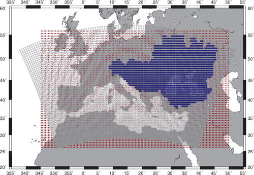
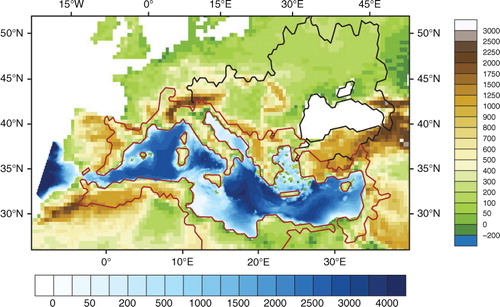
Fig. 2 ALADIN-Climate land–sea mask and orography (in m) for the Med-CORDEX domain, and NEMOMED8 bathymetry (in m). The drainage areas of the Black Sea (in black) and of the Mediterranean Sea (in red, cut North of 26°N, without the Nile basin) are contoured.

2.2. The ocean regional model NEMOMED8

The NEMOMED8 regional model (Beuvier et al., 2010) is a regional Mediterranean Sea version of the NEMO-V2.3 ocean model (Madec, 2008). NEMOMED8 covers the Mediterranean Sea plus a buffer zone including a nearby part of the Atlantic Ocean, where a 3D damping is performed to a temperature and salinity state, so that the circulation through the strait is simulated with realistic Atlantic Waters (AW). The model does not include the Black Sea. The 1/8°×1/8° cos(lat) grid is tilted and stretched at the Gibraltar Strait to follow the SW–NE axis of the strait better and to increase the local resolution up to 6 km. Elsewhere the resolution varies from 9 to 12 km from North to South. The grid has 43 vertical levels, with layer thickness increasing from 6 to 200 m. The partial steps definition of the bottom layer is used, with a no-slip lateral boundary condition on the velocity and the surface is parameterised with the free surface configuration and with the filtered formulation. The bathymetry is depicted in Fig. 2. The time step used is 1200 s.

A new feature, the relaxation of the sea surface height (SSH) in the Atlantic buffer zone, has been added to the model. This method was first implemented in NEMOMED12 (Beuvier et al., 2012). It was similarly added to NEMOMED8 (Soto-Navarro et al., 2014), with the following formula:1

where ssh is the SSH of the model, ssh_comb is the monthly value of the reference, and relax is the relaxation term which spatially varies along the longitudes. Relax is equal to 1/1.7 s from the western limit of the domain to 7.5°W; it decreases linearly to 1/90 d from 7.5°W to 6°W and is equal to zero for the rest of the domain.

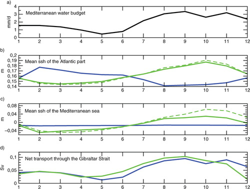
The prescribed SSH on the Atlantic side of the Gibraltar Strait will impose a signal containing the effect of steric and mass variations at global scales, allowing the volume conservation, which is not imposed in the regional model: in the previous experiments, the evaporated water of the Mediterranean basin was introduced into the Atlantic buffer zone, leading to spurious sea-level variations. Figure 3 shows the added value of the SSH relaxation by comparing two simulations with NEMOMED8 in a stand-alone mode for the 2003–2008 period, with the same set-up as in Soto-Navarro et al. (2014), except for the addition in the simulation represented in green of an SSH relaxation to the NEMOVAR-COMBINE reanalysis (Balmaseda et al., 2010) in the Atlantic part. With the relaxation, the model improves the representation of the seasonal cycle of the SSH in the Mediterranean Sea considerably, bring it close to that of the NEMOVAR-COMBINE reanalysis used as a reference. Further, the net transport through the Gibraltar Strait is better simulated, as shown by Soto-Navarro et al. (2014), especially the seasonal cycle of the inflow (not shown). It is worth noting that the mass variations at the global scale will be introduced only if they are included in the imposed SSH; that is, if the large-scale model assimilates observed SSH or contains the melting of continental ice.

Fig. 3 Seasonal cycle of (a) the Mediterranean water budget, (b) the SSH of the Atlantic part, (c) the SSH of the Mediterranean and (d) the net water transport through the Gibraltar Strait, for two NEMOMED8 2003–2008 simulations, without SSH relaxation (blue), and with SSH relaxation (solid green). The reference NEMOVAR-COMBINE is in dashed green.

The coupled version of NEMOMED8 has already been used in previous publications (Herrmann et al., 2011; Dubois et al., 2012; L'Hévéder et al., 2013; Gualdi et al., 2013a), but without the coupling of rivers. Here, the river runoffs are fully coupled from the atmospheric model to the river routing model and then to the oceanic model. All the rivers of the Mediterranean and the Black Sea drainage area are included in that way, except for the Nile river, as we will see later. There is one ocean grid-point which receives the runoffs flowing into the Black Sea added to the Evaporation minus Precipitation budget of the Black Sea. Two grid-points, Damietta and Rosetta, are used for the Nile Delta, and 230 other mouths receiving the river runoffs from the TRIP model.

2.3. The TRIP river routing model

The TRIP river routing model was developed by Oki and Sud (1998) at the University of Tokyo. It is used at Météo-France to convert the runoff simulated by the ISBA land-surface scheme into river discharge using a global river channel network at 1° or 0.5° resolutions (0.5° in this RCSM4 version) (Decharme et al., 2010; Szczypta et al., 2012; Voldoire et al., 2013). TRIP is based on a single prognostic reservoir whose discharge ( in kg/s) is linearly related to the river mass (S in kg), using a uniform and constant flow velocity (ν in m/s), equal to 0.5 m/s:2

(kg/s) represents the sum of the surface runoff from ISBA within the grid cell and the water inflow from the adjacent upstream neighbouring grid cells, (kg/s) is the deep drainage from ISBA, and L (m) the river length, which considers a meandering ratio of 1.4 as proposed by Oki and Sud (1998).

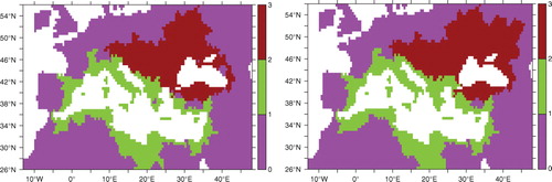
The 0.5° grid is cut on a domain that covers the whole drainage area of the Mediterranean and the Black Sea (Figs. 1 and 2), except for the Nile river basin, whose runoff is prescribed by a 12-month climatology [RivDis database, Vörosmarty et al. (1996)]. This is due to the very large size of the Nile river catchment area, which extends south of the Victoria lake, with many dams, and the fact that its current runoff is very small in comparison with the water collected all over the drainage area (Dubois et al., 2012). Ultimately, the dimensions of the domain are 122×60, with longitudes from 12.75°W to 47.75°E, and latitudes from 26.25°N to 55.75°N.

Following Ludwig et al. (2009) and Dubois et al. (2012), the TRIP 0.5° description of the flow directions has also been modified on the French and Adriatic Eastern coasts as it appeared to be unrealistic (Fig. 4), sending, for example, the Tet river on the French Roussillon coast to the Garonne drainage basin, and thus to the Atlantic Ocean instead of the Mediterranean Sea.

Fig. 4 Mediterranean (green) and Black Sea (dark red) drainage areas on the TRIP 0.5° grid, before (left) and after (right) the modifications.

2.4. The OASIS3 coupler and the coupling fields

We use the OASIS3 coupler (Valcke, 2013) with a daily coupling frequency. The wind stresses, solar and non-solar heat fluxes, and evaporation minus precipitation (E – P) budget are sent by the atmospheric model to the ocean model.

The river runoffs computed by the ISBA scheme are sent to the TRIP model, and the river discharges at the river mouths are sent by TRIP to the ocean model. Only the TRIP cells included in the Mediterranean and Black Sea drainage area are considered. The river discharges of the Black Sea drainage area (58 river mouths in the TRIP 0.5° grid) are summed with the E–P budget over the Black Sea and sent to the same ocean grid-point.

The SST field of the ocean model is sent to the atmospheric model. The ERA-Interim SST values are used for the sea points of the atmospheric model grid that are not present in the ocean grid.

3. Spin-up, initial and boundary conditions

3.1. Initial conditions and spin-up

The initial conditions of the NEMOMED8 model are set by the month of August of the 1960 year of the 10-yr filtered Rixen dataset (Rixen et al., 2005), completed with the Reynaud climatology (Reynaud et al., 1998) in the Atlantic part of the domain. We insist on the fact that this initial condition does not include any pattern which would result from the interannual variability of the Mediterranean Sea of the end of the 20th century. First, a 5-yr spin-up was computed with the NEMOMED8 model in a forced mode, with a 3D damping to the initial condition, to create the current structure without altering the water mass. Next, 21 yr of spin-up of the RCSM4 were performed with the same conditions as for the hindcast, using the 1980–1986 period in a three-time loop. The goal is to reach an ocean state representative of the beginning of the 1980s with the constraint of an ERA-Interim dataset starting in 1979. The ALADIN-Climate simulation starts from an ERA-Interim initial state for the 3D prognostic variables of the model (atmosphere, land surface). The first 2 yr are considered spin-up, allowing the land water content to reach its equilibrium. However, it is worth noting that this land-surface spin-up is negligible with respect to the coupled model spin-up.

3.2. Atmospheric lateral boundary conditions

Reanalyses of multidecadal series of past observations are used, among other things, to provide boundary conditions in the framework of long-term oceanic and atmospheric numerical hindcast simulations. The ERA-Interim reanalysis (Berrisford et al., 2009) covers the period from 1979 up to today. The ERA-Interim data assimilation system uses a 2006 release of the Integrated Forecasting System developed jointly by ECMWF and Météo-France, which contains many improvements, both in the forecasting model and in the analysis methodology relative to ERA40 (Simmons and Gibson, 2000), particularly in the resolution (T255, 80 km, http://www.ecmwf.int/research/era/do/get/era-interim). Outputs were produced every 6 hours. In the current study, ALADIN-Climate uses the full-resolution ERA-Interim 3D reanalysis as atmospheric lateral boundary conditions every 6 hours after a vertical and horizontal interpolation onto the ALADIN-Climate model grid. Land-surface parameters and aerosols concentrations are updated every month following a climatological seasonal cycle derived from observations. The sea surface temperatures are those of the ocean model over the coupled area and are updated every month outside the Mediterranean Sea with a monthly variability following ERA-Interim SSTs. In addition to lateral boundary forcings, we used the spectral nudging technique. Complete details concerning this technique can be found in Radu et al. (2008) and Colin et al. (2010). This technique allows a better constraint of the large-scales of a limited-area model that is usually driven only at its lateral boundaries. In the spectral space, a relaxation towards the driving model (here, the reanalysis) is applied to the large-scales of some of the prognostic variables. In ALADIN-Climate, the following parameters are tuneable: the choice of the nudged variables, the strength of the nudging (which depends on the variable and the altitude) and the threshold of the large-scales to be nudged. In the current study we nudged the following prognostic variables: temperature, specific humidity, wind vorticity, wind divergence and the logarithm of the surface pressure. The maximum e-folding time depends on the variables (6 hours for the vorticity, 24 hours for the logarithm of the surface pressure, the specific humidity and the temperature, 48 hours for the divergence) following the setting of Guldberg et al. (2005). The maximum e-folding time is reached above 700 hPa and for scales larger than 1280 km. The nudging decreases linearly between 700 and 850 hPa and between 1280 and 640 km for the horizontal scales. Therefore, the atmospheric boundary layer and the scales not represented in ERA-Interim are not nudged. All of this set-up is in agreement with the CORDEX recommendations for the evaluation runs except for the use of the spectral nudging technique which is not specified. A non-coupled ALADIN twin simulation forced by ERA-Interim SST, hereafter referred to as ARCM, for Atmosphere RCM, was also performed and will be used for comparison.

3.3. Oceanic lateral boundary conditions

The NEMOVAR-COMBINE reanalysis is used for the 3D damping in temperature and salinity in the Atlantic part of the domain. A reanalysis like NEMOVAR-COMBINE provides temperature and salinity conditions, and thus fluxes through the Gibraltar Strait, with an interannual variability, as opposed to a climatology such as Reynaud's. The coefficients of relaxation evolve from 3 d at the western limit of the domain to 100 d at the 7.5°W latitude, and monthly means are used from 1980 to 2008. Then, from 2009 to 2012, the year 2008 is maintained, as NEMOVAR-COMBINE is not available after 2008.

The anomalies of the SSH from the same source are used for the SSH relaxation: monthly fields are prepared as anomalies to the average SSH of a previous experiment performed without any SSH relaxation. While the NEMOVAR-COMBINE reanalysis does not include any SSH assimilation, it shows a monthly variability which is relatively realistic, though underestimated (not shown) compared to the GLORYS1V1 reanalysis (Ferry et al., 2010) which assimilates the AVISO Sea Level Anomaly (SSALTO/DUACS User Handbook, 2013).

4. Results

4.1. Air–sea fluxes evaluation

The atmospheric heat fluxes over the Mediterranean Sea represent the energy that the ocean surface receives from the atmosphere. A comparison of the different components of the heat budget is performed with different datasets. The datasets used for the evaluation are derived from the best estimates of different in-situ and/or satellite reconstructions. A selection was made from the numerous available datasets based on the following criteria: no spurious behaviour in time and space over the Mediterranean Sea, a clear land–sea mask, a 20-yr minimum common period and respect of the Gibraltar Strait long-term closure hypothesis (balance between the net heat transport through the Gibraltar Strait, the surface heat flux over the Mediterranean Sea and the heat content trend). Ultimately, only five datasets were kept. SRB-GEWEX data is produced by the NASA Global Energy and Water-cycle Experiment (GEWEX) SRB project (version 3.0), as well as SRB-QC (Quality Check), providing surface radiation at 1°×1° resolution (Stackhouse et al., 2000). The ISCCP data are part of the World Climate Research Program collecting weather satellite radiance measurements (Zhang et al., 2004; Zerefos et al., 2009). The data are global with a spatial resolution of 2.5°×2.5°. The NOCS products are based on Voluntary Observing Ships observations from the international Comprehensive Ocean–Atmosphere Data Set (Woodruff et al., 1998; Berry and Kent, 2009). We use here a NOCS version adapted to the Mediterranean Sea (Sanchez-Gomez et al. 2011; S. Josey, personal communication). The data are at 1°×1° horizontal resolution. The OAFLUX products integrate satellite observations with surface moorings, ships reports and atmospheric model reanalysed surface meteorology Yu et al., 2008), with a 1°×1° horizontal resolution. The combinations obtained by the shortwave from SRB-QC, ISCCP or NOCS, the longwave from NOCS or SRB-GEWEX, the sensible heat flux from OAFLUX or NOCS and the latent heat flux from OAFLUX or NOCS, providing that they agree with the Gibraltar Heat Transport (Béthoux, 1979; Bunker et al., 1982; Macdonald et al., 1994; Criado-Aldeanueva et al., 2012) give a range for the total heat budget of −10 to 0 W/m² over the 20-yr period from 1985 to 2004. The values of the individual components are in agreement with Pettenuzzo et al. (2010) and the HB3 estimation in Sanchez-Gomez et al. (2011).

Figure 5 and Table 1 show the annual and interannual variability for the four different terms of the heat budget in comparison with the observations. The uncertainty in the observations is represented by the spread of the average curves. The standard deviation of each dataset is not included to build an error bar, as the observations and the model cover the same period. Results of RCSM4 and the stand-alone ALADIN-Climate simulation (ARCM forced by ERA-Interim SST) are compared.

Fig. 5 Time series of yearly averaged heat fluxes in W/m² (shortwave, longwave, latent, sensible, top), their seasonal cycle (middle); total heat flux and seasonal cycle (bottom); RCSM4 in red, ARCM in blue, observations in grey; the seasonal cycles are computed over the 1985–2004 period.

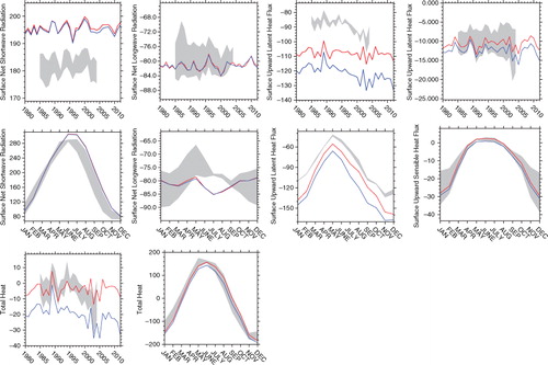
Table 1. Mean values for the shortwave, longwave, latent, sensible and total heat fluxes over the Mediterranean Sea for the 1985–2004 period in W/m²

SW	LW	Lat	Sens	Total
[178; 185]	[−84; –75]	[−90; –88]	[−14; –6]	[−10; 0]
OBS	SRB-QC, ISCCP, NOCS	NOCS, SRB-GEWEX	NOCS, OAFLUX	OAFLUX, NOCS	Combination
RCSM4	196	−81	−108	−11	−4
ARCM	196	−82	−120	−12	−19

The RCSM4 net shortwave radiation has a mean value of 196 W/m² over the 1985–2004 period, with a strong bias of more than 10 W/m² above the observations, particularly in summer. The best estimate from the observations is 178–185 W/m² on average over the 1985–2004 period using the reconstruction from SRB-QC, ISCCP and NOCS. This positive bias is similar in ARCM. The bias is higher along the African coast and in the western basin (Fig. 6a), particularly in summer. The interannual variability is well represented, with interannual correlations equal to 0.87 (0.70 and 0.60, respectively) between RCSM4 and ISCCP (resp. SRB-QC and NOCS). The net shortwave of ISCCP and SRB-QC is computed as follows:3

Fig. 6 Winter (DJF, left) and summer (JJA, right) difference (in W/m²) between RCSM4 and different observations for the 1984–2007 period.

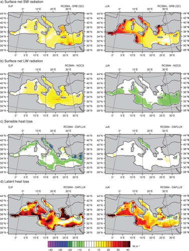
where alb is the albedo monthly values of an ocean point from ISCCP, with a mean value of 0.065, and SWdown is the downward shortwave.

For the net LW, the mean value is −81 W/m² for the 1985–2004 period for RCSM4 and −82 W/m² for ARCM simulations. These values are found to be in the range of the observations (SRB-GEWEX and NOCS). For SRB-GEWEX, the net longwave is computed as follows:4

where is the surface emissivity equal to 0.97, LWdown the downward flux, σ the Stefan-Boltzmann constant (equal to 5.67 10⁻⁸ J/s/m²/K⁴) and T the sea surface temperature (in °K) taken from Marullo et al. (2011). It is difficult to interpret the seasonality of the model bias in LW. Indeed, the amplitude and phase of the seasonal cycle of the Mediterranean surface LW are very uncertain in the various observation-based datasets that show inconsistencies like the models [Fig. 5 using SRB-GEWEX and NOCS, Sanchez-Gomez et al. (2011) and Dubois et al. (2012)]. In Sanchez-Gomez et al. (2011), the seasonal cycles of NOCS and ERA40 are very different, as are those from the 12 ARCMs analysed, showing that the seasonal cycle of the LW is still an open issue. The model seasonal cycle shows two maxima in May and December and a minimum in July/August. Those peaks are found not in the observations, but in some of the ARCMs analysed in Sanchez-Gomez et al. (2011). Fig. 6b presents a positive and relatively uniform bias in winter, and a negative bias in summer in the southern Mediterranean. The summer underestimation of LW radiation is partly explained by the dust aerosols (Nabat et al., 2014b).

For the latent heat loss, the mean value is 108 W/m² for the RCSM4 simulation and 120 W/m² for the ARCM simulation over the period 1985–2004. This value is nearly 20 W/m² greater than in the observations. Here, RCSM4 shows an added value compared to ARCM, due to a better consistency between the SST and the atmospheric fluxes. The interannual variability is captured well, but the trend observed in recent years in the observations (OAFLUX and NOCS) is not. This point as well as the strong bias will be discussed in Section 5. Note that the ARCM simulation reproduces the latent heat trend. The seasonal cycle peaks in November/ December, with a mean value of 150 W/m² associated with strong, cold and dry winds during this period; a minimum is found in May/June with a value as low as 60 W/m².

For the sensible heat flux, the mean value is the weakest term of the heat budget and is equal to 11 W/m² for the RCSM4 simulation and 12 W/m² for the ARCM simulation over the 1985–2004 period. It is found to be in the range of the observations (OAFLUX: 14 W/m² and NOCS: 6 W/m²).

Those four different terms compose the total heat budget at the ocean surface. This total net heat flux is negative (the Mediterranean Sea loses heat through the surface in average) to balance out the heat gain through the strait of Gibraltar. For the period 1985–2004, it is about −4 W/m² for the RCSM4 simulation and −19 W/m² for the ARCM simulation. The coupled simulation is of the order of magnitude of the different combinations obtained with the different datasets and in agreement with the Gibraltar Strait heat transport; this is not the case for the ARCM simulation, mainly due to the overestimated latent heat flux. The interannual variability shows heat gains in some years (e.g. 1989) and strong heat losses in others (e.g. 2005), and is very well captured by RCSM4, with the exception of the trend due to the latent heat loss, which is simulated only by ARCM.

4.2. Water, heat and salt budgets

Table 2 gives the water, heat and salt budgets of the CNRM-RCSM4 model averaged over the 1980–2012 period. The aim of this table is both to compare the input and output of water, heat and salt fluxes of RCSM4 to the observations, and to check the ability of the ocean model to close these budgets.

Table 2. Water, heat and salt budgets of the Mediterranean given by the coupled simulation and the observations

Parameter	1980–2012 mean	Observations
Water inflow at Gibraltar	0.85 Sv	0.81 (Soto-Navarro et al. 2014)
Water outflow at Gibraltar	−0.80 Sv	−0.78 Sv (ibid)
Net water flux at Gibraltar	0.05 Sv	0.04–0.10 Sv (see text)
Water flux through the surface	−0.67 m/yr or 0.05 Sv	−0.43 to – 0.66 m/yr (Sanchez-Gomez et al., 2011)
Heat flux through the surface	−5.1 W/m^2	−3 to–10 W/m^2 (see text)
Heat flux at Gibraltar	6.8 W/m^2
Heat content change	0.007°K/yr or 1.4 W/m^2
Salt transport at Gibraltar	1.10^16 g/yr or 0.003 psu/yr
Mediterranean salt content change	1.10^16 g/yr or 0.003 psu/yr
Evaporation RCSM4	1.39 m/yr	1.09 to 1.13 m/yr (Sanchez-Gomez et al., 2011)
Evaporation ARCM	1.53 m/yr
Precipitation RCSM4	0.51 m/yr	0.26 to 0.59 m/yr (ibid)
Precipitation ARCM	0.58 m/yr
E – P RCSM4	0.89 m/yr	0.50 to 0.88 m/yr (ibid)
E – P ARCM	0.95 m/yr
Runoff	0.13 m/yr
Runoff (1980–2000)	0.13 m/yr	0.13 m/yr (Ludwig et al., 2009)
Black Sea	0.09 m/yr
Black Sea (1980–1997)	0.10 m/yr	0.11 m/yr (Stanev and Peneva, 2002)

The inflow, outflow and net water transport at the Gibraltar Strait are in agreement with all the estimations found in the literature and in Beuvier et al. (2010), giving a net inflow between 0.04 and 0.10 Sv. The net water flux E–P–R–B (R for runoff and B for Black Sea) of −0.67 m/yr is at the upper limit of the observations gathered by Sanchez-Gomez et al. (2011). It is fully balanced with the net water transport at the Gibraltar Strait. Given that the observations are not on exactly the same period as the RCSM4 simulation, Table 2 shows that, when the E and P terms that comprise the E–P budget are compared with observations, the E–P budget of RCSM4 is nearly in agreement with the observations, while that of ARCM is overestimated.

The heat flux through the surface in Table 2 contains the loss due to the evaporation of surface water at the sea surface temperature with the following formula:5

where SHF is the surface heat flux (in W/m²), Q is the surface heat flux (in W/m²) received from the ALADIN-Climate model, ρ ₀ is the volumic mass of reference, equal to 1020 kg/m³ in NEMOMED8, Cp is the ocean specific heat, equal to 4000 J/kg°C, and E-P-R-B are the various terms of the water budget (in m/s). Note that the second term of the equation is computed online at each time step of the model and is an approximation of the vertical flux of heat through the surface linked with the free surface movement in NEMO. The changes in the heat and salt content are computed as the difference between the final and initial instantaneous files of the model, divided by the time between the two dates. We use these terms to characterise the heat and salt budget closure of the model, considering that the change should compensate for the difference between the surface fluxes and the Gibraltar transports. We find that the heat budget is nearly closed, with a 0.3 W/m² mismatch (Table 2). The salt transported through the Gibraltar Strait is fully balanced by the salt content change.

4.3. Comparison to buoys

Buoy datasets are key in-situ observations for validating ocean–atmosphere coupled systems. The AZUR (7.87°E, 43.42°N) and LION (4.68°E, 42.06°N) buoys from Météo-France, available since 1999 and 2002, respectively, provide long-term measurements of meteorological parameters: 2-m temperature (T2m in °C), 2-m specific humidity (Q2m in g/kg), 10-m wind speed (FF10 in m/s) and Mean Sea Level Pressure (MSLP in hPa). As for the oceanic parameter, the SST is recorded at the locations of the buoy (see Section 4.5.1). The comparison of the simulation to these two buoy datasets can only serve as an indication for the validation of the atmosphere model, because we compare a 50×50 km grid mesh to a single position. Besides, as the coupling between ALADIN-Climate and NEMOMED8 has a frequency of 1 d, there is no diurnal cycle of the surface fluxes nor, consequently, of the ocean surface layer. Therefore, we cannot compare the diurnal cycles of the parameters, only the daily means. Table 3 shows the RCSM4's ability to capture the meteorological variations well. Indeed, correlation values of 0.96 or 0.97 are found for daily MSLP, and 0.74 and 0.84 for daily air temperature, once the seasonal cycle is removed. The wind speed variations are better reproduced over the LION buoy (cor=0.9) than over the AZUR buoy (cor=0.81), and the biases for the wind speed are weak (±0.17 m/s). The weakest correlation values are found for the 2-m specific humidity (0.52 over the AZUR buoy and 0.61 over the LION buoy).

Table 3. Correlation and bias of the daily atmospheric and oceanic parameters available from the AZUR and LION buoys with the outputs of RCSM4

T2m	T2m (°C)	MSLP	MSLP (hPa)	FF10	FF10 (m/s)	Q2m	Q2m (g/kg)	SST	SST (°C)
Corr.	Bias	Corr.	Bias	Corr.	Bias	Corr.	Bias	Corr.	Bias
AZUR	0.74	0.21	0.96	0.61	0.81	0.17	0.52	3.3	0.63	0.14
LION	0.84	−0.11	0.97	0.30	0.90	−0.17	0.61	2.1	0.75	−0.52

For the correlations the seasonal cycle has been removed.

4.4. River runoffs

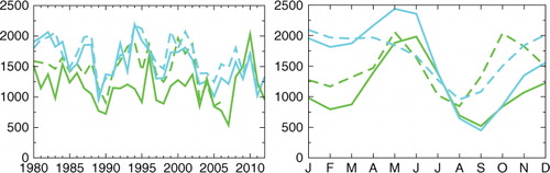
The annual runoff of the rivers in the Mediterranean Sea is highly correlated to the observations of Ludwig et al. (2009) and Stanev and Peneva (2002), with a correlation equal to 0.94, and a weak bias of 0.01 m/yr for the total inflow of freshwater during the common 1980–1997 period, due to the Black Sea, as shown in Fig. 7 and Table 2. When examining the river runoffs in greater detail, we can compare the river discharges of the TRIP model to the observations. The yearly mean of the Rhône discharge is quite accurately represented by the model (Fig. 8), with a 1980–2011 mean of 1572 m³/s, while the observations give 1680 m³/s, with a correlation equal to 0.90. However, the seasonal cycle shown in Fig. 8 is overestimated, which can be explained by the absence of dams and the representation of ground-water in the ISBA and TRIP models. The underestimation is more obvious for the Po river, with a 1980–2006 mean of 1137 m³/s compared to 1457 m³/s for the observations, but the correlation is still high, equal to 0.73. As for the Rhône river, the minimum and maximum values of the seasonal cycle are delayed by 1 month, and the underestimation of the winter season is greater than for the other seasons. These comparisons show that the model is able to simulate a realistic input of fresh water at the Mediterranean Sea scale, especially in terms of interannual variations, but performs less well at the individual river scale.

Fig. 7 Annual mean of the river runoff in the Mediterranean Sea without the Black Sea (top, mm/day) compared to the Ludwig database, of the E–P–R budget of the Black Sea (middle, mm/day) compared to the Stanev and Peneva data, and of the total inflow of freshwater (bottom, mm/day) compared to the addition of Ludwig and Stanev data.

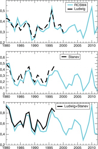
Fig. 8 Time series of the yearly river discharge (left) and mean seasonal cycle (right) in m³/s of the Rhône (blue, 1980–2011) and the Po (green, 1980–2006), observations in dashed lines.

4.5. Surface ocean characteristics

4.5.1 Sea surface temperature.

Three types of datasets are available for the evaluation of the SST: Marullo et al. (2007) provide gridded 1985–2005 fields from satellite infrared AVHRR; Ingleby and Huddleston (2007) perform a 1-degree monthly objective analysis from ocean temperature and salinity profiles called EN3; Rixen et al. (2005) offer estimations of the temperature and salinity variability from the MEDAR set of data. Here we will use the 1-yr surface average. The mean 1980–2012 RCSM4 SST field and the 1985–2007 difference with the Marullo average are presented for winter (JFM) and summer (JAS) in Fig. 9, showing a cold bias of the simulation which is more significant in the Eastern part, especially in summer. This cold bias, averaged over the whole Mediterranean basin, increases from 0.3° in 1985 to 0.8° in 2007, as shown in Fig. 10. This increase is seen only in comparison to the Marullo climatology, not with the EN3 climatology nor the Rixen dataset, for which the difference of mean Mediterranean SST of the simulation is constant. An inconsistency between the model SST and the satellite (Marullo) SST may appear, given that the latter gives night-time values (which are also corrected from skin effect). Nevertheless, the yearly mean SST of the simulation is highly correlated with the Marullo, EN3 and ERA-Interim datasets. The mean values, standard deviations and correlations computed over the relevant periods are presented in Table 4. The standard deviations are close, but slightly underestimated in RCSM4.

Fig. 9 RCSM4 SST in winter (JFM, top left), and summer (JAS, top right), averaged over the 1980–2012 period; difference between the RCSM4 SST mean and the Marullo mean climatology in winter (JFM, bottom left), and summer (JAS, bottom right), for the 1985–2007 period; SST in °C.

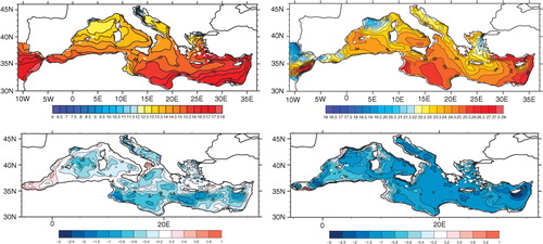
Fig. 10 Time series of the yearly mean SSS (psu, top) and SST (°C, bottom) averaged over the Mediterranean basin of RCSM4 (blue) compared to the EN3 (black dashed), Rixen (brown dashed), Marullo (red) and ERA-Interim (green) climatologies.

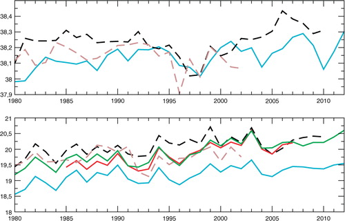
Table 4. Mean and standard deviation of the Mediterranean Sea averaged SST and SSS on the indicated periods

RCSM4	EN3	RCSM4	Rixen	RCSM4	Marullo	RCSM4	ERAI
MED basin	1980–2010	1980–2010	1980–2002	1980–2002	1985–2007	1985–2007	1980–2012	1980–2012
SST °C (std. dev.)	19.18 (0.27)	20.10 (0.30)	19.11 (0.27)	19.74 (0.26)	19.23 (0.22)	19.83 (0.35)	19.20 (0.27)	19.90 (0.38)
Correlation	0.86	0.56	0.85	0.93
SSS (psu) (std. dev.)	38.14 (0.08)	38.24 (0.09)	38.12 (0.07)	38.14 (0.08)
Correlation	0.45	0.23

The correlation is computed on the yearly means between RCSM4 and the observations.

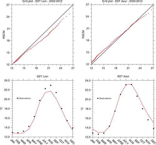
When comparing the daily SST of the ocean model grid-point corresponding to the position of the LION buoy, Fig. 11 shows a model cold bias already seen in Fig. 9 with the comparison to Marullo, equal to −0.52°C on the complete series (Table 3). This discrepancy is greater than the 0.2°C exactitude of the measurement over the period studied and is due to the underestimation of SST maxima in summer. For the AZUR position, the model tends to overestimate the SST, with a 0.14°C bias, showing an underestimation of the surface cooling in winter (Fig. 11). Once the seasonal cycle is removed, the correlations of the daily SST series are equal to 0.63 for the AZUR buoy and 0.75 for the LION buoy. For both buoy positions, the seasonal cycle amplitude of the model is slightly underestimated.

Fig. 11 Q–Q plot of the daily SST (°C) at the locations of the LION buoy (top left) and AZUR buoy (top right); seasonal cycle of the SST (bottom); observed values (dots) stand for the buoys.

4.5.2 Sea surface salinity.

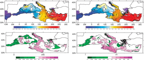
The mean 1980–2012 sea surface salinity (SSS) is presented in Fig. 12. The river mouths appear as minima of salinity, lower than on the EN3 climatology, as can be seen in the difference computed over 1980–2010 (Fig. 12). This is particularly apparent in the Aegean Sea, as the Black Sea is treated as a river in the model. Explaining the SSS bias near the river mouths is a complex issue. For one thing, the EN3 climatology has a low spatial resolution and probably suffers from sub-sampling close to the coast line. Further, the two reference datasets (EN3 and Rixen) are quite different, with a correlation equal to 0.5, and the evolution of the yearly mean of RCSM4 (Fig. 10) is also not very close. The mean values and the correlation computed on the relevant periods are presented in Table 4. There is no bias compared to Rixen, and only a small bias compared to EN3. The standard deviations are similar for the three datasets, demonstrating the coupled model's ability to represent the SSS interannual variability. As for the correlations, they are much lower than for the SST, but the observations are also less reliable, due to sampling difficulties (see Section 5).

Fig. 12 RCSM4 SSS (psu) in winter (JFM, top left), and summer (JAS, top right), averaged over the 1980–2012 period; difference between the RCSM4 SSS mean and the EN3 mean climatology in winter (JFM, bottom left), and summer (JAS, bottom right), for the 1980–2010 period.

4.5.3 SSH and circulation.

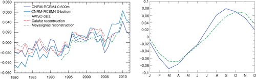
The SSH presents a particular challenge for ocean models, especially with the Boussinesq approximation as used in NEMO: the main hypothesis is the conservation of volume rather than mass. In the Mediterranean Sea, there is also the possibility of salt mass change, through the Gibraltar Strait. Jordà and Gomis (2013) show that it might induce a change of SSH of a magnitude range which compensates the SSH change related to the halosteric contribution. A first approximation for properly comparing the SSH of the model to the AVISO Sea Level Anomaly (SSALTO/DUACS, 2013) is to add only the thermosteric contribution (as a constant resulting from the average over the whole basin) to the dynamic SSH of the model. The mean dynamic SSH and circulation, and the interannual variability of the mean Mediterranean dynamic SSH plus the thermosteric contribution are plotted in Figs. 13 and 14. We also choose to compute the 0–600 m thermosteric contribution, in order to avoid a trend due to the trend in temperature in deep water (see Fig. 16). Two reconstructions of the sea level are also represented (Calafat and Jordà, 2011; Meyssignac et al., 2011). The correlation of the RCSM4 series (0–bottom) to AVISO for the 1993–2011 period is equal to 0.86 (0.68 for the detrended series). The amplitude of the mean seasonal cycle is equal to 16.9 cm for the simulation, and 14 cm for AVISO (Fig. 14). Thus, the model is able to reproduce a variability which is realistic over the years, and in terms of seasonal cycle.

Fig. 13 1980–2012 dynamic SSH (in cm) and currents at 25 m (in m/s).

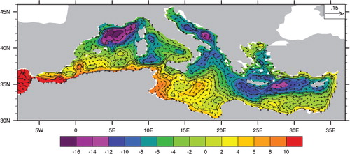
Fig. 14 Time series of mean sea-level anomalies centred on the mean of the reference period for each dataset (left, in m). For the model data, the dynamic SSH is added to the thermosteric term, which is computed over the full water column (CNRM-RCSM4 0–bottom) or the 0–600 m layer (CNRM-RCSM4 0–600 m). Model data are compared to observations (AVISO) and reconstructions (Calafat and Jordà 2011; Meyssignac et al. 2011). The model seasonal cycle is compared to AVISO data (right).

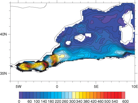
The mesoscale activity of the ocean can be characterised by Eddy Kinetic Energy (EKE). This diagnosis is particularly adapted to identifying the regions of eddies, current meanders, fronts and their variability. Pascual et al. (2014) performed a detailed analysis of the EKE of a long-term hindcast simulation performed with NEMOMED8 in a stand-alone mode over the same period of time as RCSM4. It is computed here as in Pascual et al. (2014), from the daily SSH, the anomalies with respect to the average over the whole period, and the geostrophic assumption (Fig. 15). The western basin is represented, for comparison with Fig. 3 in Pascual et al. (2014). The two Alboran Gyres are represented, with a maximum value of 520 cm²/s² over the 1993–2007 period (not shown), thus stronger than the value of 250 cm²/s² given by Pascual et al. (2014) over the same period. The Almeria Oran Front is also stronger (410 cm²/s² vs. 200 cm²/s²), as is the Northern Current (70 cm²/s² vs. 50 cm²/s²), while the Algerian Current is of the same order (up to 250 cm²/s²).

Fig. 15 Geostrophic Eddy Kinetic Energy (cm²/s²) computed from the daily SSH for the 1980–2012 period.

4.6. Ocean temperature and salinity characteristics

The yearly means of potential temperature and salinity are computed for the layers 0–150 m, 150–600 m, 600 m–bottom and the whole column (top–bottom) for the Mediterranean basin (Med), the Western and the Eastern basins (Fig. 16, without any correction of bias or trend). The temperatures and salinities of the bottom layer are plotted even though we are aware that the observations are less reliable in deep areas. As for the salinity the observation profiles are more sparse than for the temperature. For the Med basin, the correlations between the model and the EN3 climatology are high over the common periods (see Table 5), with the exception of the 0–150 m salinity, confirming the difference in SSS seen in Figs. 10 and 12. The warm bias and trend in the whole column of Med are explained by the behaviour in the bottom layer of the Eastern basin. The negative bias in the Mediterranean subsurface salinity is mostly due to the Western basin, and the positive bias and trend in salinity of the whole column come from the bottom layer of the Eastern basin. The intermediate layer (150–600 m) is well represented, with nearly no bias and a good interannual variability.

Fig. 16 Time series of Mediterranean (left), Western (middle) and Eastern Mediterranean (right) of yearly mean of salinity (in psu) and potential temperature (in °C). RCSM4, in dark blue, is compared to the Rixen climatology (uncertainty shaded in grey), and the EN3 climatology in brown. They are computed for 3 layers (0–150 m, 150–600 m, 600 m–bottom) and the whole column (top–bottom).

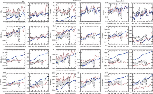
Table 5. Mean values of temperature and salinity of different layers of the Mediterranean basin for EN3, the simulation, and correlation

T3D	T3D	T3D	T3D	S3D	S3D	S3D	S3D
1980–2010	Surfaces–bottom	0–150 m	150 m–600 m	600 m–bottom	Surf–bottom	0–150 m	150 m–600 m	600 m–bottom
EN3	13.67	16.33	14.02	13.27	38.63	38.42	38.74	38.63
RCSM4	13.77	16.04	13.96	13.41	38.66	38.31	38.74	38.68
Correlation	0.86	0.92	0.78	0.68	0.73	0.45	0.67	0.69

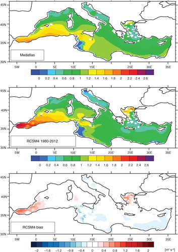
In order to illustrate the stratification of the surface layer, we compute the stratification index (IS) of the 0–150 m layer as in Herrmann et al. (2010). This corresponds to the loss of buoyancy necessary to induce convection through this layer. The higher the value of IS, the more stratified the layer. Figure 17 compares the 0–150 IS for MEDATLAS and RCSM4, as well as the bias. The Alboran region is more stratified in RCSM4 than in MEDATLAS due to (1) a weak mixing of the incoming Atlantic water through Gibraltar, and thus an excessively strong vertical density gradient in this region, and (2) because the surface layer of NEMOVAR-COMBINE is lighter compared to MEDATLAS. Another large discrepancy is found in the Aegean Sea: this may be related to the fact that we treat the Black Sea as a river, which leads to very fresh surface water close to the mouth grid-point.

Fig. 17 Stratification Index computed for the 0–150 m layer, MEDATLAS (top), RCSM4 (middle) and bias (bottom).

The 34°N section in Fig. 18 (and the line on Fig. 19) for the model and for the Rixen climatology, shows that the model agrees well with the observations in general, despite a bottom layer which is too salty and too warm, confirming results of Fig. 16.

Fig. 18 Temperature (in °C) and salinity (in psu) transects at 34°N in the Eastern basin (2 left columns) and 5°E in the Western basin (2 right columns) of RCSM4 (up) and Rixen (bottom) for the 1980–2002 period.

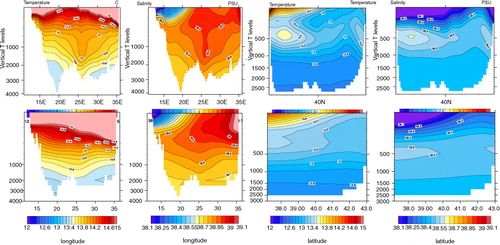
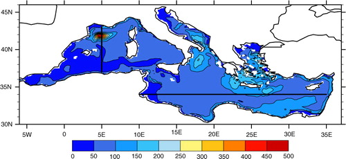
Fig. 19 1980–2012 winter (JFM) mixed layer depth (in m). 5°E and 34°N sections (lines).

The 5°E section in the Western basin (Fig. 18 and the line on Fig. 19) shows that the model represents the main characteristics of the basin quite well, with the Modified Atlantic Water (MAW, identified by a minimum of salinity at the surface on the two transects of Fig. 18), the Winter Intermediate Waters (WIW, subsurface minimum of temperature on the 5°E transect), the Levantine Intermediate Water (LIW, maximum of salinity on the 34°N transect), the Western Mediterranean Deep Water (WMDW, minimum of temperature) and the isopycnal doming in the Gulf of Lions gyre near 42°N. The LIW feature appears to be slightly amplified in RCSM4 (warmer and saltier), especially after the 1990s, in agreement with Fig. 16.

4.7. Ocean winter convection and thermohaline circulation

4.7.1. Winter convection.

Open-sea deep convection is one of the characteristics of the Mediterranean Sea. It occurs during winter, when cold and dry winds induce a cooling and densening effect of the surface water, making it sink and produce deep water through strong mixing. The main areas are the Gulf of Lions, where the WMDW is formed, the Adriatic Sea, where Eastern Mediterranean Deep Water (EMDW) is formed before overflowing through the Otranto Strait, and to a lesser extent the LIW and the Aegean Sea (Cretan Deep Water, CDW). To characterise the mixed layer depth with NEMOMED8, we use the turbocline depth: that is, the depth at which the vertical eddy diffusivity coefficient falls below a given value, equal to 5 cm/s².

The main convection regions can be found in Fig. 19, which represents the mean 1980–2012 winter (JFM) mixed layer depth. Then, for each year and each of the four sub-basins [Adriatic (ADRI, North of 40°N), Levantine (LEVA, East of 25°E), Aegean Sea (AEGE) and Gulf of Lions (LION)], we keep the temporal maximum values of the spatial maximum values of each daily mixed layer depth field (see Fig. 20a). The model shows a strong interannual variability in all the sub-basins. The evaluation of this variability is not straightforward with the existing in-situ observations, as it requires a Winter Conductivity Temperature Depth (CTD) cast, and these are sparse. For the Gulf of Lions, we can however rely on the extensive literature. We are nearly sure that open-sea deep convection (MLDmax >1000 m) occurred in the following years: 1982, 1987 and 1992 (Mertens and Schott, 1998), 1999 and 2000 (Béthoux et al., 2002), 2005 and 2006 (Schroeder et al., 2008), 2009, 2010, 2011, 2012 (L. Houpert, personal communication, using the LOCEAN-CEFREM deep mooring). Despite a strong interannual variability, CNRM-RCSM4 simulates open-sea deep convection for all the observed years, with the possible exception of 1982 (750 m for the model, 1100 m for the observations) and 1992 (750 m for the model, 1400 m for the observations). On the whole, the model simulates a convection deeper than 1000 m for 18 of the 33 yr, giving a 54% rate [see Sannino et al. (2009), Herrmann et al. (2010) and L'Hévéder et al. (2013) for other model results, ranging from 39 to 87% of convective years].

Fig. 20 a: Daily maximum each year of the mixed layer depth (in m) in the four sub-basins Adriatic Sea (ADRI), Aegean Sea (AEGE), Levantine basin (LEVA), and Gulf of Lions (LION); b: Monthly volume of water in m³ with density larger than 29.1 (black), 29.2 (red), and 29.3 (green) for ADRI, AEGE and LEVA. For LION the thresholds are 29.10 (black), 29.11 (red) and 29.12 (green); c: Formation rate in Sv for water with density greater than the same thresholds as b.

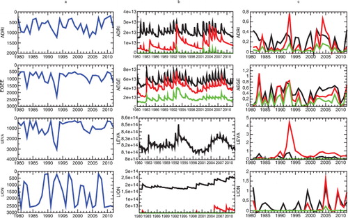
For each month, we compute the volume of water with a density greater than 29.1, 29.2 and 29.3 for ADRI, AEGE and LEVA sub-basins and 29.10, 29.11, 29.12 for LION (Fig. 20b). Then the yearly formation rate (expressed in Sv) is computed taking the maximum volume of the year and the minimum volume of the year before, divided by 1 yr in seconds (Fig. 20c). We noticed an increase in deep water volume in the Gulf of Lions from 1999 onwards, and this may be a sign of the denser LIW entering the Western basin (Schroeder et al., 2008). The years of deep convection clearly appear as years of strong formation rates. The strong formation rate during the 1992–1993 years will be discussed in Section 4.8.

4.7.2. Meridional and zonal overturning stream function.

The meridional overturning stream function (integration of the meridional circulation along the longitudes) is computed for the Adriatic and Northern Ionian sea (North of 37°N), and the zonal overturning stream function (integration of the zonal circulation along the latitudes) is computed for the Mediterranean Sea, East of the Gibraltar Strait, as in Somot et al. (2006). They show the vertical circulation of the water, and especially the main water mass circulation in the basin. Figure 21, right, shows the overflow of dense water from the Adriatic at the Otranto Strait, becoming the EMDW south of 40°N. Figure 21, left, shows the mean circulation of the surface Atlantic Water, and the westward path of the LIW in the subsurface layer. EMDW, which originates at the Aegean Sea, is outflowing at 27°E, which is characteristic of the EMT period.

Fig. 21 1980–2012 zonal overturning stream function of the MED (left), meridional overturning stream function on the Adri-Ionian basin (right), in Sv.

4.8. Eastern Mediterranean Transient

The EMT refers to the period between the late 1980s and the early 1990s, when the Aegean Sea produced very dense water which flowed into the Levantine basin to form new EMDW, replacing the deep dense water which usually flows from the Adriatic Sea. The EMT was first reported by Roether et al. (1996) and its evolution has since then been further analysed by Klein et al. (1999), Lascaratos et al. (1999), Theocharis et al. (1999) and Zervakis et al. (2004) and finally reviewed by Roether et al. (2007). The densest overflows were recorded in the deepest straits of the Cretan Arc, Kassos and Karpathos, located East of Crete (Theocharis et al., 2002; Kontoyiannis et al., 2005). After overflowing the sills of the Cretan Arc straits, the new EMDW sank to the bottom of the eastern Mediterranean and spread. Our modelling study shares the same oceanic model NEMOMED8 as in Beuvier et al. (2010), but here we have different initial conditions: we use a pre-EMT climatology to initialise the model [Beuvier et al. (2010) used MEDATLAS and mentioned the change of climatology for a pre-EMT one as a perspective of improvement], different Atlantic boundary conditions and atmospheric forcings (cf. Section 3.1). However, we will compare the chronology and the intensity of this event in the two simulations and with the observations.

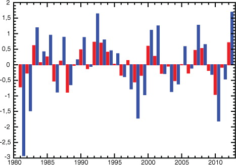
Josey (2003) described strong anomalies of winter heat and water fluxes which lead to strong density anomalies in the Aegean Sea. These anomalies, computed on NDJF months, are presented on Figs. 22 and 23. The maximum of the heat flux anomaly (−86 W/m² in 1992 and −66 W/m² in 1993), and the anomalies of E-P (+0.72 m/yr in 1992, the highest value of the period, and +0.69 m/yr in 1993) are stronger than the SOC and NCEP/NCAR in Josey (2003) (+0.5 to 0.7 m/yr for E-P, −54 to −65 W/m² for the heat flux). The NDJF anomalies of E–P–R–B equal to 1.64 m/yr in 1992 and 0.80 m/yr in 1993 also confirm the diminution of the Black Sea input during these years. The winter anomalies of heat flux are larger than in Beuvier et al. (2010) (−73 in 1992 and −65 W/m² in 1993), in contrast to the E–P–R–B winter anomalies (−0.73 in 1992 and −1 m/yr in 1993).

Fig. 22 Anomalies of winter (NDJF) surface heat flux averaged over the Aegean Sea (in W/m²).

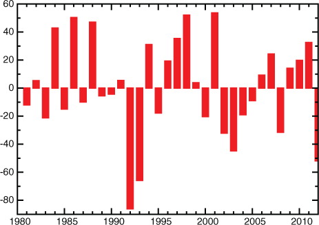
Fig. 23 Anomalies of winter (NDJF) E–P (red), and E–P–R–B (blue) averaged over the Aegean Sea (in m/yr).

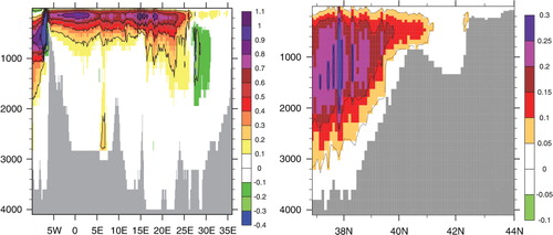
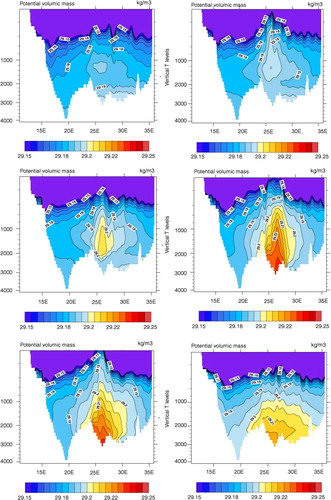
The daily maximum of mixed layer depth reaches the bottom in 1993 in the Aegean Sea and the Levantine basin (Fig. 20). The maximum rate of formation (density greater than 29.3) is reached in 1993 and is equal to 0.74 Sv, larger than the 0.55 Sv found in Beuvier et al. (2010). It is important to note that deep convection also occurred in the Adriatic Sea in 1993, showing that deep waters were still being formed during the winter of 1992–1993, but with a lower density (29.2 instead of 29.3). From Fig. 20, it is clear that the EMT in the model is a long-term accumulation process of dense water in the Aegean Sea with the formation of water denser than 29.3 in 1983, 1985, 1987, 1989, 1990, 1992 and 1993. This dense water accumulation, combined with the anomalies of surface heat fluxes and Black Sea runoff, lead to overflow through the sills of the Cretan Arc at the beginning of the 1990s with a peak of 4.5 Sv of water denser than 29.2 in 1993 in the Levantine basin (Fig. 20c). This large volume of dense water allows the CDW to reach the bottom of the Levantine Basin (see Fig. 25) after overflowing the sills. When the limit of the LEVA basin is shifted to 20°E, the Antikithera Strait is included, and the formation rate of water denser than 29.2 reaches 3.2 Sv in 1992 and 8.7 Sv in 1993 (not shown). Thus, there is also an outflow of dense water through the Antikithera Strait as found in the observations (Roether et al., 2007). The monthly values of the potential densities of the waters just above the sill of Antikithera, Kassos and Karpathos straits are compared to the observations (Fig. 24, Kontoyiannis, personal communication). For the Karpathos Strait, the model densities are higher than the observed ones, and also much higher than in Beuvier et al. (2010). But for the Kassos and Antikithera straits, the monthly chronology of the model follows the observations, and the densities are consistent. The difference of results between the Karpathos Strait on one side, and the Kassos and Antikithera straits on the other come from the difference of the depth at which the densities were obtained, in the observations and in the simulation: nearly the same depth for the first, deeper for the observations than for the model for the two others. The 34°N density sections displayed for May 1980 (beginning of the simulation), 1989 and 1991 (pre-EMT conditions), 1994, 1995 and 2000 (post-EMT conditions) in Fig. 25 show that waters denser than 29.24 kg/m³ appear in 1994 at the bottom of the Levantine basin, South of Crete. In terms of basin characteristics (Fig. 16), the signature of the EMT in the Eastern basin (cooling and freshening in the intermediate layer, warming and saltening in the deep layer due to a massive vertical reorganisation of the water masses) is important enough in the simulation to influence the whole Mediterranean. However, Figs. 16 and 18 show that the impact of the EMT signal on the long-term average is stronger in the model than in the observations.

Fig. 24 Monthly potential density (in kg/m³) simulated on the bottom of the Cretan Arc sills (lines) and observed south of the sill channels (circles).

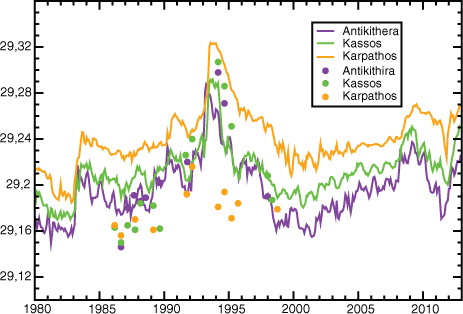
Fig. 25 Density transects for May at 34°N, for years 1980 (top left), 1989 (top right), 1991 (middle left), 1994 (middle right), 1995 (bottom left) and 2000 (bottom right).

We showed in this section that the main characteristics of the EMT event are simulated by RCSM4. The surface flux conditions are well represented, as is the formation of Aegean deep water, as well as its overflow through the Antikithera, Kassos and Karpathos straits to form new EMDW. To the best of our knowledge, reproducing the EMT with this level of accuracy has never before been achieved in a realistic long-term hindcast simulation without ad-hoc flux correction.

5. Discussion

5.1. Comparison of CNRM-RCSM4 with the state-of-the-art Mediterranean RCSMs

After the evaluation of the 1980–2012 simulation of CNRM-RCSM4, and the comparison with available observations, we choose to discuss the added value of this method compared to the previous systems, in particular for river, air–sea flux and ocean behaviours. We have to keep in mind that most of the published RCSMs were forced by the ERA-40 reanalysis (Artale et al., 2010; Herrmann et al., 2011; Carillo et al., 2012; L'Hévéder et al., 2013) or by GCMs (Somot et al., 2008; Krzic et al., 2011; Carillo et al., 2012; Dell'Aquila et al., 2012; Dubois et al., 2012; Rojas et al., 2013; Sanna et al., 2013) and that only one 5-member multi-model ensemble is available [FP6-CIRCE project, Dubois et al. (2012), Gualdi et al. (2013a)]. Note that reanalysis-driven simulations are expected to perform better than GCM-driven simulations, as their lateral boundary conditions can be considered more realistic. To our knowledge, only one simulation [Drobinski et al. (2012), Di Luca et al. (2014), same simulation] described an ERA-Interim driven RCSM for a period (1989–2008), shorter than in the current study (1980–2012). A recent review of the literature can be found in Li et al. (2012) and Planton et al. (2012).

In terms of the river runoff, CNRM-RCSM4 shows very similar performances for the Mediterranean rivers (averaged over the whole basin or for the Rhone and Po rivers) compared to previous ERA-40 driven runs (Carillo et al., 2012) and better agreement in term of biases than GCM-driven runs (Dubois et al., 2012). The Black Sea freshwater budget (E–P–R budget of the Black Sea) has clearly been improved with respect to previous simulations (Carillo et al., 2012; Dubois et al., 2012). Note that the PROTHEUS system is using an ad-hoc correction of the Black Sea freshwater budget (Dell'Aquila et al., 2012).

As for the air–sea fluxes, CNRM-RCSM4 confirms that RCSMs are able to simulate realistic a Mediterranean Sea surface heat budget thanks to atmosphere-SST consistency (e.g. Somot et al., 2008; Dubois et al., 2012; L'Hévéder et al., 2013) without consistently improving the biases in individual components of the budget (e.g. SW bias in CNRM-RCSM4). With respect to the individual components of the heat budget, the CNRM-RCSM4 simulation has biases (between +11 and +18 W/m² in SW and between +18 and +20 W/m² in LH loss with good values for LW and SH) comparable to other models. With respect to the reference datasets of Table 1 in this study, Sanchez-Gomez et al. (2011) give a bias range of [−31; +36] W/m² for the SW and of [−5; +40] for the LH loss for the Atmosphere-RCMs, and Dubois et al. (2012) a range of [−35; +26] W/m² for the SW and [−12; +10] W/m² for the LH loss for RCSMs driven by GCMs. Concerning the water budget, CNRM-RCSM4 shows better performances than most of the models in previous studies (Sanchez-Gomez et al., 2011; Dubois et al., 2012), which explains the very good behaviour of the model in SSS and salt content. The model SST cold bias is present in most of the other ERA40-driven RCSMs (Li et al., 2012) and GCM-driven RCSMs (Dubois et al., 2012; Sanna et al., 2013) except for the LMDZ-Med/NEMOMED8 model, which shows nearly no SST bias (L'Hévéder et al., 2013). However, despite spatial biases, the SSS simulated by CNRM-RCSM4 has the smallest bias on average over the Mediterranean Sea among the published RCSMs, with most of the other RCSMs showing an overestimated SSS (Carillo et al., 2012; L'Hévéder et al., 2013; Di Luca et al., 2014). The behaviours of the heat and salt contents (bias, variability, trend) of CNRM-RCSM4 are similar to the best simulations published up until now using PROTHEUS (Carillo et al., 2012), in particular those without spurious deep layer drifts leading to realistic thermosteric sea-level representation. The surface circulation has not been detailed in previously published Mediterranean RCSMs, but the surface circulation of CNRM-RCSM4 has the same qualities and drawbacks as the stand-alone ocean simulations based on the NEMOMED family (Beuvier et al., 2010, 2012). In addition, the Mediterranean deep water formations (DWF) and the Mediterranean thermohaline circulation (MTHC) are well-simulated in both Eastern and Western basins with the representation of all the open-sea DWF areas, the simulation of a stable WMDW formation with strong interannual variability, the deep overflow of the Adriatic Deep Water south of Otranto and the simulation of a realistic EMT. Even though quantitative evaluation of the DWF and MTHC is a complex issue due to the lack of long-term observations, we believe that the 1980–2012 hindcast simulation performed with the CNRM-RCSM4 model has the most realistic MTHC ever simulated at climate-scale with Mediterranean ocean models based on OPA or NEMO (Somot et al., 2006; Béranger et al., 2010; Beuvier et al., 2010, 2012; Herrmann et al., 2010; L'Hévéder et al., 2013; Pinardi et al., 2013).

5.2. Current limitations of CNRM-RCSM4

Establishing an understanding of the behaviours and biases of a coupled RCSM is an extensive undertaking, and it is beyond the scope of this study to address all of them. However, we would like to discuss some of the most striking points mentioned in Section 4.

Concerning the air–sea fluxes (see Table 1), the Mediterranean Sea surface heat budget is achieved by compensating errors with an excessively large surface shortwave (+11/+18 W/m² depending on the reference data) and excessively large latent heat loss (+18/+20 W/m²). These biases were already identified in previous studies using ALADIN in versions 4 and 5 (Sanchez-Gomez et al., 2011; Dubois et al., 2012). Further, the origin of these biases has been identified and will be corrected in the next generation of CNRM-RCSM4. In the surface shortwave, the bias is explained by two main causes: an underestimation of the aerosol effect on the surface shortwave with the Tegen aerosol climatology used in this study [the bias is reduced by 3 W/m² over the 1985–2004 period using the improved climatology developed in Nabat et al., (2013)] and a general underestimation of the cloud cover [see Fig. 2 in Nabat et al. (2014b)]. As for the LH loss bias, it is partially explained by the use of the spectral nudging technique, as a sensitivity test using ALADIN-Climate without spectral nudging gives a 9 W/m² weaker latent heat loss for the 1985–2004 period (not shown). The remaining bias is most probably due to the use of the Louis (1979) bulk formula to compute the turbulent fluxes. Indeed this formula is known to overestimate the latent heat flux by strong wind conditions (S. Belamari and G. Caniaux, personal communication). The next generation of CNRM-RCSM4 will use a more recent bulk formula adapted to Mediterranean Sea conditions. A sensitivity test using ALADIN-Climate with the ECUME bulk formula (Belamari, 2005) instead of the Louis reduces the LH loss by 19 W/m² (not shown).

Another hypothesis concerning the LH loss overestimation is a possible overestimation of the surface wind speed. Herrmann et al. (2011) and Nabat et al. (2014b) showed that ALADIN-Climate and CNRM-RCSM4 simulate a sea surface wind speed in agreement with the QuikSCAT satellite product with a slight underestimation of the upper-quantile. This result is confirmed by the comparison of the model surface wind speed with the AZUR and LION buoys (cf. Section 4.3). We conclude that the representation of the surface wind speed may not cause the latent heat loss overestimation in CNRM-RCSM4. As for the estimation of the surface wind speed, Herrmann et al. (2011) proved that the dynamical downscaling of ERA-Interim gives better results than using ERA-40 and also that the use of the spectral nudging technique leads to better daily correlation, especially in the eastern part of the basin. Both options were used in the current set-up. Following Herrmann et al. (2011), we expect a mean bias to QuikSCAT lower than −14%. Additionally, humidity at 2 m is overestimated with respect to buoy observations as a consequence of the excessively large LH loss and thus cannot be considered as a possible cause of the LH bias. As seen in Table 1, while the surface net heat budget of CNRM-RCSM4 (−4 W/m²) is in agreement with the observed estimates ([−10; 0] W/m²) over the period 1985–2004, this is not the case of the non-coupled ALADIN-Climate twin simulation, which shows an overestimated surface net heat loss (−19 W/m²). The difference between both simulations explains the cold SST bias in CNRM-RCSM4, as the SST of the coupled model cools until the equilibrium between the Gibraltar net flow and the surface heat loss is nearly reached. Note that this balance is always achieved in Mediterranean RCSMs (e.g. Somot et al., 2008; Dubois et al., 2012). To achieve this balance, the latent heat flux is modified from −120 W/m² in ALADIN to −108 W/m² in CNRM-RCSM4. Knowing that the averaged model SST bias is equal to −0.9°C or −0.6°C depending on the reference dataset (see Table 4), we can compute the average air–sea flux/SST retroaction coefficient of the model, which is equal to [−17; −25] W/m²/K. Despite its spatial and temporal variations (not computed here), this retroaction coefficient can be compared to the relaxation coefficient used in stand-alone ocean models for SST relaxation. For example, in the NEMOMED8 simulations (e.g. Beuvier et al., 2010; Herrmann et al., 2010), −40 W/m²/K is used.

For the Mediterranean Sea water budget, estimates of precipitation over the sea remain inconsistent (e.g. Sanchez-Gomez et al., 2011) limiting the possibility of evaluating this component of the water budget. However, we believe that precipitation over the sea is overestimated in CNRM-RCSM4, as both the precipitation over land (see Nabat et al., 2014b) and the evaporation are overestimated. The river runoff discharges are well represented, with a weak deficit of 0.01 m/yr for the total runoff in the Mediterranean Sea compared with the observed estimates (due to the Black Sea freshwater input). The interannual variability of the total Mediterranean river runoff discharge is captured very well by RCSM4, with a correlation of 0.94. This means that the lack of human influence (dams, irrigation) in the current version of the ISBA land model and TRIP river model is not detrimental to simulating the interannual scale. The seasonal cycle is, however, difficult to capture in CNRM-RCSM4 (see for example Fig. 8). This can be attributed to the following causes: the seasonal cycle of the precipitation or evaporation biases over land, the misrepresentation of the underground water phenomena or the lack of human activities such as damming or irrigation in the model. It has recently been shown that the new version of TRIP (not yet included in CNRM-RCSM), which contains ground-water processes (Vergnes and Decharme, 2012; Vergnes et al., 2012), improves the seasonal cycle and in particular the summer minimum values.

The Gibraltar Strait and the related incoming AW play a key role in the Mediterranean Sea circulation (Sannino et al., 2009), in particular through the surface water stratification. Concerning the representation of the AW, Soto-Navarro et al. (2014) showed that NEMOMED8 in a forced mode reproduces the water characteristics and the volume transport of the inflow at the Gibraltar Strait well (0.80 Sv in the model vs. 0.81 Sv in the observations). Nevertheless, in the current simulation in coupled mode, the incoming flux is slightly larger (0.85 Sv) and fresher. This difference comes from the change of the dataset used in the Atlantic buffer zone [NEMOVAR-COMBINE reanalysis in the current study instead of Reynaud climatology in Soto-Navarro et al. (2014)]. As the 0–150 m layer in NEMOVAR-COMBINE is less dense on average than the Reynaud climatology in the near-Atlantic (not shown), the incoming waters are consequently lighter than the observed references in the Alboran area: the model is indeed slightly warmer (Fig. 9), clearly fresher (Fig. 12) and too stratified (Fig. 17). Note that we consider the newly used NEMOVAR-COMBINE dataset to be more realistic than the previous, older Reynaud dataset. In particular, thanks to data assimilation, the reanalysis includes the evolution of the Atlantic water mass characteristics related to climate change (not shown). The behaviour of CNRM-RCSM4 is thus probably related to deficiencies in water mixing at the AW/MOW interface at the strait of Gibraltar, where no specific parameterisation is applied.

One of the goals of the design of CNRM-RCSM4 is to represent all the forcings of the SSS variability, which is not the case in stand-alone regional ocean models and previous RCSMs. No constraint, such as correction or relaxation, is used at the air–sea interface, and evaporation and precipitation are provided daily by the high-resolution ARCM. The river discharges and the Black Sea freshwater inputs are computed online from the atmosphere precipitation over land and also provided daily. Further, we have included the monthly variability of the near-Atlantic conditions (temperature, salinity, SSH). Note, for example, that the Atlantic buffer zone salinity of the surface layer (0–150 m) has an interannual standard deviation equal to 0.08 psu. Finally, the model simulates an averaged SSS in very good agreement with the reference datasets Rixen and EN3 with nearly no bias (see Table 4), and very similar interannual standard deviations (0.08 psu for Rixen, 0.07 for EN3 and 0.08 for CNRM-RCSM4, see also Fig. 10). Note that all the other Med-CORDEX RCSMs underestimate the variability of the SSS averaged over the Mediterranean Sea (not yet published).

Nevertheless, we also must note that the SSS interannual variability in the observation-based gridded products is less reliable than the SST variability, mostly due to larger sampling errors for salinity reconstruction (Llasses et al., 2014) and to the lack of accuracy (too recent, poor spatial coverage, weak precision) of the satellite products based on SMOS for the Mediterranean Sea (Font et al., 2012). This lack of reliability in the gridded products can be illustrated by the weak interannual correlation between the EN3 and Rixen datasets (0.50 for the common period 1980–2002). Evaluating the temporal chronology of the model is therefore complex. The correlation between the SSS interannual time series of CNRM-RCSM4 and the Rixen data is only 0.23 with no determination of which is correct, the data or the model. Using 3-yr filtered time series as advised by M. Rixen (personal communication) notably improves the correlation, which reaches 0.75, limiting the sampling error effect.

Despite the weak interannual correlation between the three datasets, the SSS minimum values in 1996–1998 are well reproduced by all the datasets including the model (anomalies of about 0.15–0.20 psu with respect to the beginning of the 1990s). From the analysis of the various sources of salinity forcing in the model, we conclude that this minimum period is explained by exceptional precipitation (not shown) and river runoff (Fig. 7) values in 1996 and 1997. The total sea surface water budget E–P–R–B is thus at its minimum during these years, leading to a minimum in the net transport through the Gibraltar Strait, associated with a minimum of salt transport (not shown). Note that no salinity minimum is observed in the near-Atlantic at the same time, nor before, demonstrating that the anomaly of the water budget is the principal explanation.

The absence of a recent and high-resolution SSS gridded dataset including sampling error bars for the Mediterranean Sea limits the model evaluation, especially for its spatial patterns. Some localised biases are however clear in coastal areas (Aegean Sea, Adriatic Sea, Gulf of Gabes, shelf of the Gulf of Lions) where tide mixing, river discharge and exchange with the Black Sea (no time lag for the river discharges of the whole drainage area) have the largest influence. Too weak a mesoscale activity in CNRM-RCSM4, which is eddy-permitting and not eddy-resolving, could partly explain the spatial patterns of the salinity bias (see for example the Gulf of Lions or the Adriatic Sea in Fig. 12).

Longer term, we hope that improved gridded products with sampling error quantification, a new generation of satellite-derived products and long-term time series at buoy locations (SSS is now measured at the LION and AZUR buoys since September 2012) will increase the robustness of SSS evaluation in future modelling works.

Finally, we found that the open-sea deep convection phenomena is well represented by the model (areas of convection, depth, interannual variability, decadal variability with the EMT). However, DWF in the Mediterranean Sea is also related to another phenomena, often called shelf cascading, as in the Northern Adriatic, the Aegean Sea or the shelf of the Gulf of Lions. We would like to underline that this phenomena is currently not well represented by climate-scale ocean models with Z-levels and using 50-km atmosphere forcing such as NEMOMED8 in the CNRM-RCSM4. To be simulated correctly, some conditions must be full-filled: first, the resolution of the wind-field must be at least 10 km over the area of interest, as demonstrated for the Bora events in the Adriatic Sea (Pullen et al., 2003; Herrmann et al., 2011). Secondly, the ocean models must use either very high spatial and vertical resolution if using Z-levels (Langlais et al., 2009) or sigma coordinates (Herrmann and Somot, 2008). We hope that the next generation of RCSMs will be able to reproduce and study this Mediterranean phenomena involved in DWF and the related MTHC.

5.3. Evaluation and understanding of trends in RCSMs

The evaluation and understanding of the trends in a RCSM is an interesting but complex issue. For one thing, observations are not always sufficiently reliable, especially over the sea (Jordà and Gomis, 2013; Llasses et al., 2014), due to sampling errors or issues of temporal homogeneity. For example, the 3D-averaged salt content trend is nearly impossible to evaluate with state-of-the-art observations. We can only note that CNRM-RCSM4 shows a similar trend (+0.003 psu/yr, 1980–2012 period) as in L'Hévéder et al. (2013) (+0.002 psu/yr, 1958–2001 period) and higher than in the observations (Fig. 16). As for the 3D-averaged heat content that can be evaluated through the sea level, the model seems to overestimate the positive trend with a value of +0.008°C/yr due to an excessively large trend below 600 m (Fig. 14). This trend is two times larger than in Carillo et al. (2012) and L'Hévéder et al. (2013), which report +0.004°C/yr and +0.0045°C/yr on the 1958–2001 period, respectively. The trend is equal to 0.003 and 0.004 in Rixen (1980–2002) and EN3 (1980–2010).

The question of the SST trend and the related latent heat loss trend over the Mediterranean area has a stronger observational basis. To our knowledge, it was first illustrated using various observed datasets by Mariotti (2010) despite large uncertainties in the observed datasets. She attributed the LH loss increasing trend at the first order to the Mediterranean SST increasing trend. She also concluded that the sign of the trend is reproduced by the CMIP3 models, which is not the case for the amplitude (one order of magnitude too small in the global models). CNRM-RCSM4 clearly does not reproduce any of those trends correctly (see Figs. 5 and 10). In addition, it was recently shown that none of the Med-CORDEX coupled RCMs driven by ERA-Interim were able to reproduce the observed SST and LH trends (figure not published yet, C. Dubois, personal communication). Note, however, that the ERA-Interim reanalysis and also the ARCM ALADIN-Climate (see Fig. 5), both driven by observed SST, reproduce a strong LH trend. This confirms the key role played by the SST trend as driver of the LH trend. We can quantify these trends over the period 1985–2007 for the SST, and 1985–2004 for the LH loss. For RCSM4, the SST trend is equal to +0.13°C/decade, while it is equal to +0.39°C/decade for Marullo and to +0.33°C/decade for ERA-Interim. The LH loss trend is equal to +0.61 W/m²/yr in OAFLUX and +0.34 W/m²/yr in NOCS. These values give an estimate of the observation uncertainty. Over the same period, the coupled model CNRM-RCSM4 shows a clear underestimated trend with +0.15 W/m²/yr, whereas the corresponding Atmosphere-RCM driven by observed SST gives a value of +0.61 W/m²/yr equal to the OAFLUX value. In addition, a very recent study performed at CNRM (Nabat et al., 2014a) concludes that the Mediterranean SST trend is partly explained by the decreasing sulphate aerosol trend from the 1980s (known as the European brightening effect). Including this aerosol trend in CNRM-RCSM4 allows the improvement of the simulated SST trend as well as the SST trend spatial pattern and the related LH trend. However, even in this new simulation, the LH trend remains underestimated. The work by Nabat et al. (2014a) was not available at the time of writing this manuscript; therefore, the sulphate aerosol trend is not taken into account in CNRM-RCSM4 in the current study. Note that the observed references showing a very strong trend (−10 W/m² between 1985–1995 and 2000–2004) are also doubtful, especially the satellite-derived products which sometimes suffer from temporal breaks (Mariotti, 2010) and could be reassessed in the coming years by using new observation-based products with climate-approved quality checks and homogenisation procedures (see for example the CCI initiative of ESA, http://www.esa-cci.org/).

Concerning the SSS, a significant trend is also obtained over the 1980–2012 period in CNRM-RCSM4 (+0.005 psu/yr). In the model, this positive trend can be attributed to the lateral advection of a similar trend of the near-Atlantic Ocean (+0.005 psu/yr in average over the surface layer: 0–150 m). Note that this SSS trend is not associated to an increase in net surface water budget neither to an increase in the net Gibraltar Strait mass transport. This underlines the key role of near-Atlantic salinity variability on the Mediterranean salinity.

6. Conclusion and future improvements

The design of a new fully coupled regional climate system model (CNRM-RCSM4) dedicated to the study of Mediterranean climate variability is described and the ocean component of the model is evaluated in-depth including the analysis of ocean forcings (near-Atlantic ocean, river runoff, Black Sea freshwater inputs and air–sea fluxes). The atmospheric component has been evaluated in a companion paper (Nabat et al., 2014b). The model includes the regional representation of the atmosphere (ALADIN-Climate model), the land-surface and hydrology (ISBA model), rivers (TRIP model) and the ocean (NEMOMED8 model) with a daily coupling by the OASIS coupler. The results from a 1980–2012 hindcast simulation for which the RCSM is laterally driven by the global reanalyses are analysed. When possible, the outputs of the model are compared to the available climatologies and observations as well as to the corresponding non-coupled ARCM when relevant. For the first time, using only available satellite and in-situ datasets (ISCCP, SRC-QC and SRB-GEWEX, NOCS, OAFLUX) for a 20-yr period (1985–2004), we establish observed estimates of the various components of the Mediterranean Sea heat budget which are consistent with the Gibraltar Strait closure hypothesis. The value of the sensible heat flux (more than 100% error between the datasets), the amplitude and phase of the seasonal variations of the LW, and the representation of the aerosols in the SW and LW still remain uncertain. Our approach is based on only a selection of published datasets. The great uncertainty of precipitation over the sea does not allow the closure of the Mediterranean Sea water budget.

With respect to the published literature and to the previous generation of the CNRM coupled RCSMs, the main novelties of the CNRM-RCSM4 design are:

• the use of spectral nudging in ALADIN-Climate: this technique strongly constrains the synoptic chronology of the atmospheric flow and thus the chronology of the air–sea fluxes and of the ocean response. This facilitates day-to-day and interannual evaluation with respect to relevant observations. It also limits the internal variability of the atmosphere RCM;

• the use of global ocean reanalysis to drive the near-Atlantic buffer zone including interannual variability for temperature, salinity and sea level. This allows the Mediterranean SSS interannual variability to be improved and the climate trends in the near-Atlantic ocean to be taken into account;

• the use of a SSH relaxation in the near-Atlantic region instead of the water conservation hypothesis. This allows improvement of the seasonal cycle of the Mediterranean Sea level;

• the interactive coupling of Mediterranean and Black Sea river runoff without correction through the use of the river routine scheme TRIP and a parameterisation of the Black Sea freshwater inputs. This allows us to close the regional water budget and make the Mediterranean salinity consistent with the precipitation over land. The Nile discharge is prescribed with observed values;

• the use of a 26-yr long spin-up;

• the use of new initial conditions representative of the 1960s, thus excluding the effect of the EMT;

• no correction or relaxation at any of the interfaces between the ocean, atmosphere, land surface, surface hydrology and rivers, allowing the spatio-temporal variability of the system to be maximised.

The CNRM-RCSM4 model is able to reproduce the main features of the Mediterranean Sea with respect to observed references. Taking into account the observation limitations, the average behaviour, the seasonal cycle and the interannual variability of the SST, SSS, sea level, surface circulation, total heat and salt content, net heat and water budget, river runoff discharges, Gibraltar Strait exchanges and ocean deep convection in various sub-basins are well reproduced by the model. With regards to the Mediterranean Sea thermohaline circulation, the EMT, the overflow of the Adriatic Sea deep water, south of the Otranto Strait and the strong interannual variability of the WMDW formation are particularly well captured with respect to the current knowledge obtained from observations. Demonstrating the added value of the RCSM with respect to Atmosphere-only RCM and Ocean-only RCM is difficult and is not the main focus of this study. However, we showed that the latent heat loss, the surface net heat budget and the surface net water budget of the Mediterranean Sea are better simulated using the RCSM than the corresponding ARCM, probably due to the improved atmosphere-SST consistency. The main drawbacks of the hindcast simulation are an overestimation of the surface shortwave and latent heat loss, a cold bias in SST, especially in summer, an excessively fresh bias in the surface layers of the Western Mediterranean Sea, leading to surface layers which are too stratified and a Gibraltar Strait inflow which is too strong. CNRM-RCSM4 also shows deficiencies in reproducing observed trends for some of the ocean-related variables. At the surface, the SST increase and the related latent heat loss trend are not reproduced. Despite the low reliability of the observations in the ocean bottom layers, we also consider that the model shows an overestimation of the bottom layer trends in temperature and salinity in the Eastern Mediterranean Sea. This last bias leads to a slightly overestimated trend of the heat and salt content of the whole Mediterranean Sea and consequently of the thermosteric sea level.

In addition to the above-mentioned biases, the main limitations of the current CNRM-RCSM4 set-up are the relatively low resolution of the atmosphere model [50 km whereas 12 km models are now available for the Mediterranean area, Herrmann et al. (2011), Tramblay et al. (2013)], the relative low resolution of the ocean model (10 km), which can be considered as eddy-permitting and not eddy-resolving for the Mediterranean Sea [whereas 2-km resolution Mediterranean Sea models are now available (Soto-Navarro et al., 2014)], a lack of representation of the SST and air-sea fluxes diurnal cycle, an overly simple representation of the exchanges between the Black Sea and Aegean Sea, an overly simple representation of the Gibraltar Strait (Sannino et al., 2009; Soto-Navarro et al., 2014) and finally the lack of online representation and coupling of other key components of the Mediterranean climate system such as aerosols (Nabat et al., 2013), ocean biogeochemistry [to improve the solar radiation penetration, Palmiéri et al. (2014)], waves, or the human influence on the river runoff (dams, irrigation and water management).

Despite the aforementioned model biases and modelling limitations, we consider that the in-depth evaluation of the atmospheric component (Nabat et al., 2014b) and of the river and ocean components (this study) of CNRM-RCSM4 as well as the good performance of the model in simulating the present climate variability allow its behaviour to be validated in hindcast mode driven by reanalyses. CNRM-RCSM4 will be used in the future for detailed analyses of the past variability of Mediterranean climate using sensitivity studies in hindcast mode, for regional climate change future projections in the framework of CORDEX and for multi-model intercomparisons in Med-CORDEX [www.medcordex.eu, Ruti et al. (2014)].

Acknowledgements

This work is a contribution to the HyMeX program (HYdrological cycle in the Mediterranean EXperiment) through INSU-MISTRALS support and the Med-CORDEX initiative (COordinated Regional climate Downscaling EXperiment – Mediterranean region). This research has received funding from the French National Research Agency (ANR) project REMEMBER (contract ANR-12-SENV-001) and from the European Commission as part of its 7 ^th Framework Program (CLIM-RUN, contract FP7-ENV-2010-265192).

The model version presented here is used in the projects FP7 IMPACT2C (grant 282746) and ANR ASICS-MED (contract ANR-12-BS06-0003). The outputs of the simulation described in this work can be downloaded from the Med-CORDEX database (www.medcordex.eu). The NEMOVAR-COMBINE reanalysis was produced under the FP7 COMBINE project (Grant Agreement number 226520).

We thank Marie-Noëlle Bouin and Sophie Belamari, who provided the LION and AZUR buoy datasets and participated in our discussions in this work of comparison, and Jonathan Beuvier for his corrections.

We thank W. Ludwig for the Mediterranean river datasets, E. Stanev for the Black Sea freshwater data, S. Marullo for his SST satellite products, M. Rixen for the 3D ocean climatology, B. Rossow and A. Romanou for the ISCCP data, P. Stackhouse for the SRB data, L. Yu for the OAFLUX data, S. Josey for the NOCS data and H. Kontoyiannis for the densities at the Antikithera, Kassos and Karpathos straits.

The altimeter products were produced by SSALTO/DUACS and distributed by Aviso, with support from CNES (http://www.aviso.oceanobs.com/duacs/).

References

- Artale V. , Calmanti S. , Carillo A. , Dell'Aquila A. , Herrmann M. , co-authors . An atmosphere ocean regional climate model for the Mediterranean area: assessment of a present climate simulation. Clim. Dynam. 2010; 35(5): 721–740.
- Balmaseda M. A. , Mogensen K. , Molteni F. , Weaver A. T . The NEMOVAR-COMBINE Ocean Re-Analysis. Technical Report 1. 2010. COMBINE Technical Report (ISSN 2221-1128).
- Belamari S . Report on uncertainty estimates of an optimal bulk formulation for surface turbulent fluxes. MERSEA IP Deliverable, D4.1.2. 2005; 29.
- Béranger K. , Drillet Y. , Houssais M. N. , Testor P. , Bourdallé-Badie R. , co-authors . Impact of the spatial distribution of the atmospheric forcing on water mass formation in the Mediterranean Sea. J. Geophys. Res. Oceans. 2010; 115(C12):
- Berrisford P. , Dee D. , Fielding K. , Fuentes M. N. , Kallberg P. , co-authors . The ERA-interim archive. ERA Report Series. 2009; 1: 1–16.
- Berry D. I. , Kent E. C . A new air-sea interaction gridded dataset from ICOADS with uncertainty estimates. Bull. Am. Meteorol. Soc. 2009; 90: 645–656.
- Béthoux J.-P . Budgets of the Mediterranean Sea. Their dependence on the local climate and on the characteristics of the Atlantic waters. Oceanol. Acta. 1979; 2: 157–163.
- Béthoux J.-P. , de Madron X. D. , Nyffeler F. , Tailliez D . Deep water in the Western Mediterranean: peculiar 1999 and 00 characteristics, shelf formation hypothesis, variability since 1970 and geochemical inferences. J. Mar. Syst. 2002; 33: 7–131.
- Beuvier J. , Béranger K. , Lebeaupin-Brossier C. , Somot S. , Sevault F. , co-authors . Spreading of the Western Mediterranean Deep Water after winter 2005: time scales and deep cyclone transport. J. Geophys. Res. 2012; 117
- Beuvier J. , Sevault F. , Herrmann M. , Kontoyiannis H. , Ludwig W. , co-authors . Modeling the Mediterranean Sea interannual variability during 1961–2000: focus on the Eastern Mediterranean Transient. J. Geophys. Res. 2010; 115: C08017.
- Bougeault P . A simple parameterization of the large-scale effects of cumulus convection. Mon. Weather Rev. 1985; 113(12): 08–2121.
- Bunker A. F. , Charnock H. , Goldsmith R. A . A note of the heat balance of the Mediterranean and Red Seas. J. Mar. Res. 1982; 40: 73–84.
- Calafat F. M. , Jordà G . A Mediterranean sea level reconstruction (1950–2008) with error budget estimates. Global Planet. Change. 2011; 79(1–2): 118–133.
- Carillo A. , Sannino G. , Artale V. , Ruti P. M. , Calmanti S. , co-authors . Steric sea level rise over the Mediterranean Sea: present climate and scenario simulations. Clim. Dynam. 2012; 39: 2167–2184.
- Colin J. , Déqué M. , Radu R. , Somot S . Sensitivity study of heavy precipitation in limited area model climate simulations: influence of the size of the domain and the use of the spectral nudging technique. Tellus A. 2010; 62: 591–604.
- Criado-Aldeanueva F. , Soto-Navarro J. , García-Lafuente J . Seasonal and interannual variability of surface heat and freshwater fluxes in the Mediterranean Sea: budgets and exchange through the Strait of Gibraltar. Int. J. Climatol. 2012; 32: 6–302.
- Decharme B. , Alkama R. , Douville H. , Becker M. , Cazenave A . Global evaluation of the ISBA-TRIP Continental Hydrological System. Part II: Uncertainties in river routing simulation related to flow velocity and groundwater storage. Bull. Am. Meteorol. Soc. 2010; 11: 601–617.
- Dell'Aquila A. , Calmanti S. , Ruti P. , Struglia M. V. , Pisacane G. , co-authors . Effects of seasonal cycle fluctuations in an A1B scenario over the Euro-Mediterranean region. Clim. Res. 2012; 2: 135.
- Di Luca A. , Flaounas E. , Drobinski P. , Lebeaupin-Brossier C . The atmospheric component of the Mediterranean Sea water budget in a WRF multi-physics ensemble and observations. Clim. Dynam. 2014; 43(9–10)): 2349–2375.
- Drobinski P. , Anav A. , Brossier C. L. , Samson G. , Stéfanon M. , co-authors . Model of the Regional Coupled Earth system (MORCE): application to process and climate studies in vulnerable regionsm. Environ. Model. Software. 2012; 35: 1–18.
- Dubois C. , Somot S. , Carillo S. C. A. , Déqué M. , Dell'Aquila A. , co-authors . Future projections of the surface heat and water budgets of the Mediterranean Sea in an ensemble of coupled Atmosphere-Ocean Regional Climate Models. Clim. Dynam. 2012; 39(7–8): 1859–1884.
- Farda A. , Déqué M. , Somot S. , Horanyi A. , Spiridonov V. , co-authors . Model ALADIN as regional climate model for Central and Eastern Europe. Studia Geophysica et Geodaetica. 2010; 54: 313–332.
- Ferry N. , Parent L. , Garric G. , Barnier B. , Jourdain N. C. , co-authors . Mercator Global Eddy Permitting Ocean Reanalysis GLORYS1V1: Description and Results. 2010; Technical Report, Mercator Ocean Quarterly Newsletter.
- Font J. , Boutin J. , Reul N. , Spurgeon P. , Ballabrera-Poy J. , co-authors . SMOS first data analysis for sea surface salinity determination. Int. J. Remote Sens. 2012; 34(9–10): 3654–3670.
- Geleyn J.-F . Interpolation of wind, temperature and humidity values from model levels to the height of measurement. Tellus A. 1988; 40: 347–351.
- Gualdi S. , Somot S. , Li L. , Artale V. , Adani M. , co-authors . The CIRCE simulations: a new set of regional climate change projections performed with a realistic representation of the Mediterranean Sea. Bull. Am. Meteorol. Soc. 2013a; 94: 65–81.
- Gualdi S. , Somot S. , May W. , Castellari S. , Déqué M. , co-authors . Navarra A. , Tubiana L . Future climate projections. Regional Assessment of Climate Change in the Mediterranean. 2013b; Springer Netherlands 53–118.
- Guldberg A. , Kaas E. , Déqué M. , Yang S. , Thorsen S. V . Reduction of systematic errors by empirical model correction: impact on seasonal prediction skillm. Tellus A. 2005; 57(4): 575–588.
- Haugen J. E. , Machenhauer B . A spectral limited-area model formulation with time dependent boundary conditions applied to the shallow-water equations. Mon. Weather Rev. 1993; 121: 2618–2630.
- Herrmann M. , Sevault F. , Beuvier J. , Somot S . What induced the exceptional 2005 convection event in the northwestern Mediterranean basin? Answers from a modeling study. J. Geophys. Res. Oceans. 2010; 115: C12051.
- Herrmann M. , Somot S . Relevance of ERA40 dynamical downscaling for modeling deep convection in the Mediterranean Sea. Geophys. Res. Lett. 2008; 35: L04607.
- Herrmann M. , Somot S. , Calmanti S. , Dubois C. , Sevault F . Representation of spatial and temporal variability of daily wind speed and of intense wind events over the Mediterranean Sea using dynamical downscaling: impact of the regional climate model configuration. Nat. Hazards Earth Syst. Sci. 2011; 11: 1983–2001.
- Ingleby B. , Huddleston M . Quality control of ocean temperature and salinity profiles – historical and real-time data. J. Mar. Syst. 2007; 65: 158–175.
- Jordà G. , Gomis D . On the interpretation of the steric and mass components of sea level variability: the case of the Mediterranean basin. J. Geophys. Res. Oceans. 2013; 118(2): 953–963.
- Josey S . Changes in the heat and freshwater forcing of the eastern Mediterranean and their influence on deep water formation. J. Geophys. Res. 2003; 108(C7): 1–18.
- Klein B. , Roether W. , Manca B. , Bregant D. , Beitzel V. , co-authors . The large deep water transient in the Eastern Mediterranean. Deep-Sea Res. 1999; 46: 371–414.
- Kontoyiannis H. , Balopoulos E. , Gotsis-Skretas O. , Pavlidou A. , Assimakopoulou G. , co-authors . The hydrology and biochemistry of the Cretan Straits (Antikithira and Kassos Straits) revisited in the period June 1997–May 1998. J. Mar. Syst. 2005; 53(14): 37–57.
- Krzic A. , Tosic I. , Djurdjevic V. , Veljovic K. , Rajkovic B . Changes in climate indices for Serbia according to the SRES-A1B and SRES-A2 scenarios. Clim. Res. 2011; 49: 73–86.
- Langlais C. , Barnier B. , Molines J. , Fraunié P. , Jacob D. , co-authors . Evaluation of a dynamically downscaled atmospheric reanalyse in the prospect of forcing long term simulations of the ocean circulation in the Gulf of Lions. Ocean Model. 2009; 30: 270–286.
- Lascaratos A. , Roether W. , Nittis K. , Klein B . Recent changes in deep water formation and spreading in the Eastern Mediterranean Sea: a review. Prog. Oceanogr. 1999; 44: 5–36.
- L'Hévéder B. , Li L. , Sevault F. , Somot S . Interannual variability of deep convection in the Northwestern Mediterranean simulated with a coupled AORCM. Clim. Dynam. 2013; 41(3–4): 937–960.
- Li L. , Casado A. , Congedi L. , Dell'Aquila A. , Dubois C. , Elizalde A. , co-authors . Lionello P . Modelling of the mediterranean climate system. The Climate of the Mediterranean Region, From the past to the future. 2012; London, GB and Waltham, USA: Elsevier. 419–448.
- Llasses J. , Jordà G. , Gomis D . Skills of different hydrographic networks to capture changes in the Mediterranean Sea at climate scales. Clim. Res. 2014
- Louis J.-F . A parametric model of vertical eddy fluxes in the atmosphere. Boundary Layer Meteorol. 1979; 17: 187–202.
- Ludwig W. , Dumont E. , Meybeck M. , Heussner S . River discharges of water and nutrients to the Mediterranean and Black Sea: major drivers for ecosystem changes during past and future decades?. Prog. Oceanogr. 2009; 80: 199–217.
- Macdonald A. , Candela J. , Bryden H . Seasonal and Interannual Variability of the Western Mediterranean Sea, Chapter An estimate of the net heat transport through the Strait of Gibraltar. 1994; AGU, Coastal Estuarine Studies 46. 13–32.
- Madec G . NEMO Ocean Engine. 2008; Technical Report, Paris, France, IPSL.
- Mariotti A . Recent changes in the Mediterranean water cycle: a pathway toward long-term regional hydroclimatic change?. J. Clim. 2010; 23: 1513–1525.
- Mariotti A. , Dell'Aquila A . Decadal climate variability in the Mediterranean region: roles of large-scale forcings and regional processes. Clim. Dynam. 2012; 38: 1129–1145.
- Marullo S. , Artale V. , Santoleri R . The SST multidecadal variability in the Atlantic-Mediterranean region and its relation to AMO. J. Clim. 2011; 24(16): 4385–4401.
- Marullo S. , Nardelli B. B. , Guarracino M. , Santoleri R . Observing the Mediterranean Sea from space: 21 years of Pathfinder- AVHRR sea surface temperatures (1985 to 2005): re-analysis and validation. Ocean Sci. 2007; 3: 299–310.
- Mertens C. , Schott F . Interannual variability of deep-water formation in the northwestern Mediterranean. J. Phys. Oceanogr. 1998; 28(7): 1410–1424.
- Meyssignac B. , Calafat F. M. , Somot S. , Rupolo V. , Stocchi P. , co-authors . Two-dimensional reconstruction of the Mediterranean sea level over 1970–2006 from tide gage data and regional ocean circulation model outputs. Global Planet. Change. 2011; 77(1–2): 49–61.
- Morcrette J.-J . Description of the Radiation Scheme in the ECMWF Model. 1989; Technical Report, ECMWF.
- Nabat P. , Somot S. , Mallet M. , Chiapello I. , Morcrette J. J. , co-authors . A 4-D climatology (1979–2009) of the monthly tropospheric aerosol optical depth distribution over the Mediterranean region from a comparative evaluation and blending of remote sensing and model products. Atmos. Meas. Tech. 2013; 6: 1287–1314.
- Nabat P. , Somot S. , Mallet M. , Sanchez-Lorenzo A. , Wild M . Contribution of anthropogenic sulfate aerosols to the changing Euro-Mediterranean climate since 1980. Geophys. Res. Lett. 2014a; 41: 937–960.
- Nabat P., Somot S., Mallet M., Sevault F., Chiacchio M., co-authors. Direct and semi-direct aerosol radiative effect on the Mediterranean climate variability using a coupled Regional Climate System Model. Clim. Dynam. 2014b. Online at: http://rd.springer.com/article/10.1007/s00382–014–2205–6.
- Noilhan J. , Mahfouf J.-F . The ISBA land surface parameterisation scheme. Global Planet. Change. 1996; 13: 145–159.
- Noilhan J. , Planton S . A simple parameterisation of land surface processes for meteorological models. Mon. Weather Rev. 1989; 117: 536–549.
- Oki T. , Sud Y. C . Design of total runoff integrating pathways (TRIP). A Global River Channel Network. Earth Interact. 1998; 2: 1–36.
- Palmiéri J. , Orr J. C. , Dutay J. C. , Béranger K. , Schneider A. , co-authors . Simulated anthropogenic CO2 uptake and acidification of the Mediterranean Sea. Biogeosci. Discuss. 2014; 11: 6461–6517.
- Pascual A. , Vidal-Vijandel E. , Ruiz S. , Somot S. , Papadopoulos V . Borzelli G. E. , Gacic M. , Lionello P. , Malanotte-Rizzoli P . Spatio-temporal variability of the surface circulation in the Western mediterranean: a comparative study using altimetry and modelling. The Mediterranean Sea: Temporal Variability and Spatial Patterns. 2014; Washington, USA: AGU monograph. 5–24. Technical Report, .
- Pettenuzzo D. , Large W. G. , Pinardi N . On the corrections of ERA-40 surface flux products consistent with the Mediterranean heat and water budgets and the connection between basin surface total heat flux and NAO. J. Geophys. Res. Oceans. 2010; 115(C6):
- Pinardi N. , Zavatarelli M. , Adani M. , Coppini G. , Fratianni C. , co-authors . Mediterranean Sea large-scale low-frequency ocean variability and water mass formation rates from 1987 to 2007: a retrospective analysis. Prog. Oceanogr. 2013
- Planton S. , Lionello P. , Artale V. , Aznar R. , Carillo A. , co-authors . Lionello P . The climate of the mediterranean region in future climate projections. The Climate of the Mediterranean Region, From the past to the future. 2012; London, GB and Waltham, USA: Elsevier Science Ltd. 449–502.
- Pullen J. , Doyle J. D. , Hodur R. , Ogston A. , Book J. W. , co-authors . Coupled ocean-atmosphere nested modeling of the Adriatic Sea during winter and spring 2001. J. Geophys. Res. 2003; 108(C10):
- Radu R. , Déqué M. , Somot S . Spectral nudging in a spectral regional climate model. Tellus A. 2008; 60: 898–910.
- Reynaud T. , Legrand P. , Mercier H. , Barnier B . A new analysis of hydrographic data in the Atlantic and its application to an inverse modeling study. Int. WOCE Newslett. 1998; 32
- Ricard J.-L. , Royer J.-F . A statistical cloud scheme for use in an AGCM. Ann. Geophys. Atmos. Hydrosph. Space Sci. 1993; 11: 95–1115.
- Rixen M. , Beckers J. M. , Levitus S. , Antonov J. , Boyer T. C. , co-authors . The Western Mediterranean Deep Water: a proxy for climate change. Geophys. Res. Lett. 2005; 32(12): L12608.
- Roether W. , Klein B. , Manca B. , Theokaris A. , Kioroglou S . Transient Eastern Mediterranean Deep Waters in response to the massive dense-water output of the Aegean Sea in 1990s. Prog. Oceanogr. 2007; 74: 540–571.
- Roether W. , Manca B. , Klein B. , Bregant D. , Georgopoulos D. , co-authors . Recent changes in Eastern Mediterranean Deep Waters. Science. 1996; 271: 333–334.
- Rojas M. , Li L. Z. , Kanakidou M. , Hatzianastassiou N. , Seze G. , co-authors . Winter weather regimes over the Mediterranean region: their role for the regional climate and projected changes in the twenty-first century. Clim. Dynam. 2013; 41(3–4): 551–571.
- Ruti P. , Somot S. , Dubois C. , Calmanti S. , Ahrens B. , co-authors . MED-CORDEX initiative for Mediterranean Climate studies. 2014. BAMS (submitted).
- Sanchez-Gomez E. , Somot S. , Josey S. A. , Dubois C. , Elguindi N. , co-authors . Evaluation of Mediterranean Sea water and heat budgets simulated by an ensemble of high resolution regional climate models. Clim. Dynam. 2011; 37: 2067–2086.
- Sanna A. , Lionello P. , Gualdi S . Coupled atmosphere ocean climate model simulations in the Mediterranean region: effect of a high-resolution marine model on cyclones and precipitation. Nat. Hazards Earth Syst. Sci. 2013; 13(6): 1567–1577.
- Sannino G. , Herrmann M. , Carillo A. , Rupolo V. , Ruggiero V. , co-authors . An eddy-permitting model of the Mediterranean Sea with a two-way grid refinement at the Strait of Gibraltar. Ocean Model. 2009; 30(1): 56–72.
- Schroeder K. , Ribotti A. , Borghini M. , Sorgente R. , Perilli A. , co-authors . An extensive western Mediterranean deep water renewal between 2004 and 2006. Geophys. Res. Lett. 2008; 35(18): L18605.
- Simmons J. , Gibson J . The ERA40 Project Plan. ERA40 Project Report Series, n. 1. 2000; UK, ECMWF: Reading.
- Smith R. N. B . A scheme for predicting layer clouds and their water content in a general circulation model. Q. J. Roy. Meteorol. Soc. 1990; 116: 435–460.
- Somot S. , Sevault F. , Déqué M . Transient climate change scenario simulation of the Mediterranean Sea for the twenty-first century using a high-resolution ocean circulation model. Clim. Dynam. 2006; 27: 851–879.
- Somot S. , Sevault F. , Déqué M . Design and first simulation with a tri-coupled AORCM dedicated to the Mediterranean study. Research activities in atmospheric and oceanic modelling (Blue Book) CAS/JSC Working group on numerical experimentation (WGNE). Report N. 2009; 39: 9–5.
- Somot S. , Sevault F. , Déqué M. , Crépon M . 21st century climate change scenario for the Mediterranean using a coupled atmosphere ocean regional climate model. Global Planet. Change. 2008; 63: 112–126.
- Soto-Navarro J. , Somot S. , Sevault F. , Beuvier J. , Criado-Aldeanueva F. , co-authors . Evaluation of regional ocean circulation models for the Mediterranean Sea at the Strait of Gibraltar: volume transport and thermohaline properties of the outflow. Clim. Dynam. 2014
- SSALTO/DUACS User Handbook. (M)SLA and (M)ADT near-real time and delayed time products. 2013. Nomenclature: SALP-MU-P-EA-21065-CLS. Issue 3, Rev. 4. Reference: CLSDOS-NT-06-034.
- Stackhouse P. W. , Gupta S. K. , Cox S. J. , Chiacchio M. , Mikovitz C . Smith W. L. , Timofeyev Y. M . The WCRP/GEWEX surface radiation budget project release 2: an assessment of surface fluxes at 1 degree resolution. International Radiation Symposium 2000: Current Problems in Atmospheric Radiation. 2000; Russia: St. Petersburg.
- Stanev E. V. , Peneva E. L . Regional sea level response to global climatic change: Black Sea examples. Global Planet. Change. 2002; 32: 33–47.
- Szczypta C. , Decharme B. , Carrer D. , Calvet J.-C. , Lafont S. , co-authors . Impact of precipitation and land biophysical variables on the simulated discharge of European and Mediterranean rivers. Hydrol. Earth Syst. Sci. 2012; 16: 3351–3370.
- Tegen I. , Hollrig P. , Chin M. , Fung I. , Jacob D. , co-authors . Contribution of different aerosol species to the global aerosol extinction optical thickness: estimates from model results. J. Geophys. Res. 1997; 102: 23895–23915.
- Theocharis A. , Klein B. , Nittis K. , Roether W . Evolution and status of the Eastern Mediterranean Transient (1997–1999). J. Mar. Syst. 2002; 33–34(11): 91–116.
- Theocharis A. , Nittis K. , Kontoyiannis H. , Papageorgiou E. , Balopoulos E . Climatic changes in the Aegean Sea influence the Eastern Mediterranean thermohaline circulation (1986–1997). Geophys. Res. Lett. 1999; 26(11): 1617–1620.
- Tramblay Y. , Ruelland D. , Somot S. , Bouaicha R. , Servat E . High-resolution Med-CORDEX regional climate model simulations for hydrological impact studies: a first evaluation of the ALADIN-Climate model in Morocco. Hydrol. Earth Syst. Sci. 2013; 17: 3721–3739.
- Valcke S . The OASIS3 coupler: a European climate modelling community software. Geosci. Model Dev. 2013; 6: 3–388.
- Vergnes J.-P. , Decharme B . A simple groundwater scheme in the TRIP river routing model: global off-line evaluation against GRACE terrestrial water storage estimates and observed river discharges. Hydrol. Earth Syst. Sci. 2012; 16: 3889–3908.
- Vergnes J.-P. , Decharme B. , Alkama R. , Martin E. , Habets F. , co-authors . A simple groundwater scheme for hydrological and climate applications: description and offline evaluation over France. J. Hydrometeorol. 2012; 13(4): 1149–1171.
- Voldoire A. , Sanchez-Gomez E. , Salas y Mélia D. , Decharme B. , Cassou C. , co-authors . The CNRM-CM5.1 global climate model: description and basic evaluation. Clim. Dynam. 2013; 40(9–10): 2091–2121.
- Vörosmarty C. , Fekete B. , Tucker B . Global River Discharge Database, RivDis. 1996. Technical Report, UNESCO. International Hydrological Program, Global Hydrological Archive and Analysis Systems.
- Woodruff S. D. , Diaz H. F. , Elms J. D. , Worley S. J . COADS Release 2 and metadata enhancements of marine surface flux fields. Phys. Chem. Earth. 1998; 23: 517–526.
- Yu L. , Jin X. , Weller R. A . Multidecade Global Flux Datasets from the Objectively Analyzed Air-sea Fluxes (OAFlux) Project: Latent and Sensible Heat Fluxes, Ocean Evaporation, and Related Surface Meteorological Variables. 2008; Technical Report, Woods Hole Oceanographic Institution OAFlux Project Technical Report (OA-2008–01).
- Zerefos C. S. , Eleftheratos K. , Meleti C. , Kazadzis S. , Romanou A. , co-authors . Solar dimming and brightening over Thessaloniki, Greece, and Beijing, China. Tellus B. 2009; 61(4): 657–665.
- Zervakis V. , Georgopoulos D. , Karageorgis A. , Theocharis A . On the response of the Aegean Sea to climatic variability: a review. Int. J. Climatol. 2004; 24: 1845–1858.
- Zhang Y. C. , Rossow W. B. , Lacis A. A. , Oinas V. , Mishchenko M. I . Calculation of radiative fluxes from the surface to top of atmosphere based on ISCCP and other global data sets: refinements of the radiative transfer model and the input data. J. Geophys. Res. 2004; 109(D19):