Modelling background error correlations with spatial deformations: a case study

Abstract

A long-term goal in variational data assimilation is to improve the anisotropy of background error correlations. One way to achieve anisotropic correlations is to introduce spatial deformations. This deformation can be specified a priori for instance by using the geostrophic transform (GT) as introduced by Desroziers (1997). The deformation can also be estimated from a purely statistical point of view (Michel, 2013a). The aim of this study is to evaluate the performance of such spatial deformation techniques for the use of background error modelling. A large ensemble of variational assimilations with perturbed observations is set up on a case study with the global ARPEGE model. An anisotropy index and a length scale diagnostic are defined to compare objectively the effectiveness of the deformations. This effectiveness is measured as the ability of the inverse spatial deformations to make the correlations more isotropic or more homogeneous. The results are shown to depend on the vertical level and on the variable. Generally, the statistical deformation is able to reduce the anisotropy while the GT is giving much smaller improvements that are, in this case study, confined to the frontal area of an extratropical cyclone.

• data assimilation
• anisotropy
• background error
• ensemble
• spatial deformation

1. Introduction

In Numerical Weather Prediction (NWP), the analysis step aims to estimate the best initial conditions for the next forecast by assimilating observations. Due to the lower number of observations compared to the model grid size, one usually resolves a full rank problem by using a short-range forecast called the background. The uncertainty of the background is taken into account by the background error covariance matrix B. As reviewed by Bannister (2008), most operational centres use a control variable transform (CVT). A square root of B is conveniently modelled as a sequence of transforms: the balance operator accounting for the cross-covariances between variables and the spatial transform accounting for the covariances for every unbalanced control variable. The spatial transform is also usually split in three components: the variances, the vertical and the horizontal correlations. This paper is focusing on horizontal correlations.

The variances of the background errors are the diagonal terms of B. In the ARPEGE assimilation scheme, they are estimated from a small ensemble of forecasts (currently six members in AEARP ) (Raynaud et al., 2011) and thus they are flow-dependent. The correlations are still modelled in a static way with a diagonal matrix in spectral space. This modelling yields homogeneous and isotropic correlations on the sphere (Courtier et al., 1998). To increase the heterogeneity in time and space, Varella et al. (2011) model the correlations with a diagonal matrix now in wavelet space computed over a 3-week calibration period. It was shown to improve the heterogeneity of the modelled correlations, in particular by modelling larger length scales in tropical areas and smaller length scales in mid-latitude areas. The correlation modelled with the isotropic wavelets (Fisher, 2004) do allow for heterogeneity, but only weak anisotropy.

Alternatively (or in a complementary way), spatial deformations have been proposed to model the heterogeneity and the anisotropy of the correlations. A first class of methods is attempting to model the flow dependency of the correlation with an a priori formulation of the deformation (hereafter physical approaches). For example, Benjamin (1989) proposes an isentropic vertical transform. Desroziers (1997) adapts a coordinate change, the geostrophic transform (hereafter GT) inspired from the semi-geostrophic formalism (Hoskins and Bretherton, 1972; Hoskins, 1975).

The estimation of the statistical deformation used in this paper is part of the second class of methods where the deformation is estimated over an ensemble. As in Michel (2013b), and Michel (2013a), the image processing shape from texture algorithm (Clerc and Mallat, 2002) is adapted to objectively model heterogeneity of background error correlations from the statistics of an ensemble of forecasts. This algorithm is named hereafter the statistical transform (ST).

Spatial deformations have a moderate computational cost (e.g. one interpolation) and fit well in the classical CVT formalism, such that they are good candidates for background error modelling. However, any correlation function is generally not the deformation of a stationary one, as studied by Perrin and Senoussi (1999). Thus, it is legitimate to check whether the spatial deformation introduces useful anisotropy in the structure functions. A slightly different point of view is employed in this paper: heterogeneity and anisotropy of the correlations are compared between the physical (deformed) space and the computational (inverse) space. The aim of the paper is to document the differences of anisotropies and heterogeneities between direct and inverse spaces on a case study, using objective measures.

The paper is organised as follows: in Section 2, the two methods to estimate the deformation are described. The developments implemented for this study and the setup of the experiments are explained in Section 3. Results of the ST are objectively compared with those of the GT in Section 4. Summary and discussions are given in Section 5.

2. Spatial deformations

2.1. The statistical transform

Clerc and Mallat (2002) introduce a wavelet-based algorithm capable of statistically estimating the deformation of a stationary process from a single realisation (with application to image processing). Michel (2013b) proposes to use this algorithm to model the non-stationary and anisotropy properties of the spatial correlations. This assumes that the background errors (after normalisation by their standard deviations) are well represented by spatial deformations of a spatially stationary process. Michel (2013b) also shows that the algorithm to estimate the deformation can rely on local measures of length scales (Pereira and Berre, 2006) rather than wavelets, with very similar results. Michel (2013a) applies the algorithm to the modelling of background error correlations for a convective scale model and finds that the deformed correlations have anisotropy properties close to the raw correlations. For the sake of completeness, this section is a summary of the formalism of the ST as introduced in Clerc and Mallat (2002) and Michel (2013a).

Clerc and Mallat (2002) study deformed processes defined as F(x) =R(d(x)), where and d is a function from to . In the rest of the article, we will work in two dimensions of space (n=2). Information about deformed processes is gained from a continuous wavelet analysis, which is computed as the inner product where is the spatial position and S a warping matrix that determines the shape and orientation of the wavelet. A key result from Clerc and Mallat (2002) is that such wavelet analyses of F and R can be related through a migration property:1

which is valid only for vanishing warping matrices det( S )→0 and where J _d is the Jacobian of the deformation d. Because the assumption is made that R is a spatially stationary process, its wavelet analysis does not depend on the position (in a statistical sense). More precisely, the warpogram is defined to be the variance in wavelet space:2

Following Clerc and Mallat (2002), the u-derivatives of the warpogram of R vanish, while using the migration property the warpogram of F follows the so-called texture gradient equation:3

and where the coefficients c _i,j are defined by:4

The ST algorithm thus follows these steps:

• given some realisations of F, compute their wavelet transforms;

• compute an estimate of the warpogram, the variance in wavelet space;

• compute spatial and scale derivatives of this warpogram (using for instance smoothed finite differences);

• estimate the slopes in wavelet space v _i,j from a least-square solution of the texture gradient eq. (3).

The slopes in wavelet space v _i,j are directly related to the Jacobian of the deformation:5

The term that is estimated from the wavelet analysis is known as the ‘deformation gradient’. More precisely it is the relative spatial variations of the Jacobian in the two spatial directions, whereas one would like to estimate the deformation itself. The solution was introduced by Michel (2013a), who shows that it is possible to recover the deformation from the deformation gradient by solving two elliptic partial differential equations complemented with appropriate boundary conditions. In this paper, Dirichlet conditions on the perturbations are used. This means that the deformation will not affect the boundaries of the domain. After this step, it is also possible to compute an approximate inverse deformation d ⁻¹ to be applied on F to recover the process .

This method estimates the deformation d relying on variances computation in wavelet space. The robustness of this estimate obviously depends on the sampling. In Clerc and Mallat (2002), the deformation is estimated from a single realisation of F and the sampling proposed uses several scales and wavelet orientations, as well as the use of spatial averaging. In the context of data assimilation, the structure of background errors is usually estimated over ensembles. In Michel (2013a) and in this paper, the sampling over scales and orientations is enriched by an ensemble of realisations (an ensemble of 90 forecasts) of F. For the same purpose of increasing the robustness of the estimated deformation, a spatial smoothing of the derivatives of the wavelet coefficient variances is applied. This is done with recursive filters (Purser et al., 2003a) that convolve fields with a Gaussian kernel defined by a chosen filter length L. In this study a fourth-order recursive filter (with a single sweep) is used. Values of L are discussed in Section 3.5. All other settings of the ST are the same as in Michel (2013a).

The model assumes that it is reasonable to represent background error correlations by the deformation of a homogeneous isotropic correlation model. Michel (2013b) argues that this is probably better than the usual assumption that background error correlations can be represented by a (quasi-) homogeneous isotropic correlation model (Derber and Bouttier, 1999; Berre, 2000). However, it was not proven whether these assumptions of homogeneity and isotropy hold better in computational (inverse) space. This is studied in Section 4, where the behaviour of the GT proposed by Desroziers (1997) is also described.

2.2. The geostrophic transform

The use of the GT in data assimilation is (loosely) justified from a physical point of view, rather than from a statistical point of view. Hoskins (1975) introduces a set of equations under the geostrophic momentum approximation that are related to the more common quasi-geostrophic equations by a transformation of the horizontal coordinates. This transformation is more capable of describing the formation of fronts than the quasi-geostrophic system, yet the solutions they produce are very similar from a conceptual point of view (e.g. they only differ by a deformation). The formulation of the coordinate change (x,y,z,t)→(X,Y,Z,T) to pass in transformed space is given as (Hoskins, 1975):

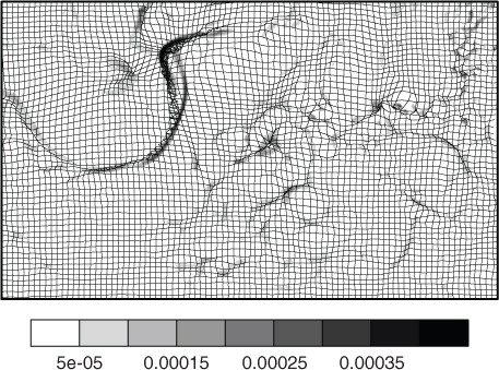
with f the Coriolis parameter and (u _g , v _g ) are the components of the geostrophic wind. The direction of the coordinate transform is orthogonal to the geostrophic wind. One property of the coordinate change estimated with GT is to increase the horizontal resolution of frontal areas in transformed space (Nordeng, 1998), which induces a stretching of the (x,y) grid-lines [in transformed space compared to the regular grid (X,Y)] along these zones. As an illustration, Fig. 1, shows the superposition of vorticity map and a regular grid bent by the deformation d estimated with the GT (here without any spatial filtering). Positive values of vorticity are associated with a compression of the grid (e.g. lower values of the Jacobian determinant of the deformation). The bending is pointing perpendicularly to the frontal axis.

Fig. 1 Relative vorticity (shadings, s ⁻¹) in the ARPEGE analysis of the 7th of November 2011 (12UTC) at model level 60 (≈900 hPa). Also shown is the Geostrophic Transform, represented here as grid lines bending of a regular grid induced by the GT (solid black lines). The geographical contours are not represented for clarity but the domain is the same as in Fig. 2.

Desroziers (1997) suggests that this transform of the horizontal coordinates could be used in data assimilation to improve the analysis in frontal areas. The coordinate change proposed by Desroziers (1997) is inspired by the semi-geostrophic theory but differs by many aspects:

• the coordinate transform is extended to the sphere by introducing an empirical relaxation of the Coriolis factor near the equator;

• the coordinate transform is applied on model level, which are based on a hybrid sigma-pressure coordinate scheme rather than height;

• an iterative spatial filtering scheme is introduced to filter out some small-scale phenomena in the transform;

• the geostrophic-wind components are approximated by the components of the non-divergent part of the wind.

The transform of the horizontal coordinates proposed by Desroziers (1997) thus differs significantly from the original geostrophic coordinates introduced by (Hoskins, 1975), yet it will still be named the ‘GT’.

The GT has been implemented in the variational assimilation scheme of the Met-Office (Semple, 2001). It was confirmed on several meteorological situations that the GT increases the flow dependency of the structure functions in baroclinic areas with especially a stretching of the correlations along fronts and cyclonic areas. The overall meteorological impact was found to be both small and neutral in terms of forecasts scores. Some cases show an improvement of the precipitation rate during the forecast. But the overall improvements do not appear clearly enough in this context to justify an operational implementation.

The computation of the GT in this paper follows the choices of Desroziers (1997). First, a relaxed Coriolis parameter has been used to avoid issues in near–equator areas. θ is the latitude, θ ₀=15° and Ω the earth spinning speed. The geostrophic wind is approximated by the non-divergent wind. The transform is applied on model levels. Some horizontal filtering is also introduced (see Section 3.5). As we are working with ensembles, one more choice has to be made whereas the GT is using the mean wind or a different wind for each member of the ensemble. In this paper, the second choice has been chosen to avoid the averaging and smoothing of the transformation in areas of interest (frontal areas for example) that could be due to displacement errors between members of the ensemble.

2.3. Link between the transport and the deformation

In the Kalman Filter equations, the background error covariance matrix is obtained from the propagation in time of the analysis error covariance matrix (plus the model error covariance matrix). The statistical framework suggested here uses a deformation of a stationary model. Therefore, there is an analogy between the deformation and the wind that deforms covariances in geophysical flows. Snyder et al. (2003) show that in a quasi-geostrophic model, the structure of forecast errors in potential vorticity is dominated by the transport (advection of reference-flow PV by the error velocity). In the cases where transport is the dominating process in the tangent-linear model, it may be particularly valid to model to background error covariances as deformation (transport) of the original background error covariance matrix. In reality however, the structure of the background error covariance and correlation also depends on other factors such as the quality and density of the observation network (Bouttier, 1994; Hamill et al., 2002) and generally on the regime of the flow.

The aim of this paper is to expand the study of Michel (2013a) by applying the ST and the GT on a new ARPEGE case study, on a wide domain for all vertical levels and variables to qualify and to quantify the possible improvements in anisotropy and heterogeneity brought by the deformation.

3. Experimental design

3.1. The meteorological situation

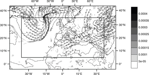
The meteorological situation is on the 7th of November 2011, 12UTC. As shown in Fig. 2, the main feature occurring is an active front over the Atlantic. It has a wide meridian extension. A strip of strong low-level vorticity characterises the cold front. The low pressure area associated with this frontal feature is below 970 hPa. The upper level dynamics (300 hPa) is also strong with a jet stream northward along the front with wind speeds around 70 m.s⁻¹. This situation of the 7th of November 2011 is also noticeable for a case of Medicane (Chaboureau et al., 2012) over the Mediterranean Sea. The signature of this cyclonic system is visible in the Western Basin of the Mediterranean Sea (40N, 6E) as a vorticity vortex at 900 hPa (Fig. 2).

Fig. 2 Map of the meteorological situation of the 7th of November 2011 (12UTC) from the ARPEGE analysis. Vorticity (shadings, 10⁻⁴s⁻¹) at model level 60 (≈900 hPa), sea surface pressure (dashed lines every 5 hPa) and winds at model level 35 (≈300 hPa) (only values over 60 kt, drawn in wind barbs). The large rectangle delimits the computational domain.

The transforms have been implemented in a Cartesian system. Thus, this study is using a large size domain extending from North American coast to Middle East. The fields used in this study are bi-dimensional and are obtained from a conformal projection. This means that the notion of anisotropy of the structure functions is the same as on the sphere. The large extension of the domain enables to see the ability of the algorithm to tackle several types of features (front, Medicane, etc.). Then it allows us to see if the ST is going to locally stationarise areas around each feature or if the stationarisation is going to be globally applied over the whole domain. Moreover, it allows one to see if the stationarisation induced by the ST on a domain much wider than the strongly anisotropic areas (frontal area for example) will undeform the correlation function to a globally lower anisotropy, instead of the high anisotropy of the concerning areas. The extension of the actual computational domain is represented by the large rectangle in Fig. 2.

3.2. The ARPEGE ensemble

Météo–France runs a six–member ensemble data assimilation system, which consists of four dimensional assimilation (4D–VAR) with explicitly perturbed observations, and implicitly perturbed analyses and backgrounds through the cycling (Berre and Desroziers, 2010). This study uses a 90-member ensemble of ARPEGE four-dimensional assimilations and forecasts. The ensemble has been cycled during 12 days from the 30th to the 8th of November 2011. Every day, four 4D–VAR assimilation cycles were done at 00, 06, 12, 18UTC, each time followed by a 6-hour forecast. The spectral resolution of every member is T399, which represents a spatial resolution of approximately 27 km. The model has 70 hybrid sigma-pressure coordinate vertical levels. For various reasons, including the neglect of model error, such ensembles generally underestimate the variance of background errors. In order to counterbalance the underestimation of dispersion of the ensemble, an on-line inflation (≈10%) of the ensemble perturbations has been applied during each cycle, as described by Raynaud et al. (2012) but including the humidity variable. This ensemble was run for the need of the HYMEX program (Ducrocq et al., 2013) that studies high impact weather events in the Mediterranean (like the Medicane).

3.3. Methodology

To evaluate the impact of the spatial deformations, the sample correlations of the ensemble in physical space (before the deformation) are compared with the sample correlations of the same ensemble but in transformed space (after the deformation). The improvements given by the deformations are quantified by the decrease of the anisotropy and heterogeneity between physical space and transformed space. The steps of the methodology are:

• Estimation of the geostrophic and statistical deformations from the ensemble in physical space.

• Applying the inverses of the geostrophic and statistical deformations to obtain the undeformed ensembles in transformed space.

• Quantifying and comparing anisotropies of the ensembles in physical and transformed space.

The estimation of the geostrophic and statistical deformations is covered in Sections 2.1 and 2.2. The framework used in this paper stays close to the one proposed by Desroziers (1997), where the deformation and its inverse are computed with a semi-Lagrangian advection scheme. Less than 10 iterations were necessary for convergence of the semi-Lagrangian advection scheme. The method to measure anisotropies is described next.

3.4. Diagnostics of anisotropy and heterogeneity

Bouttier (1993) uses the inertia matrix M of the correlation function to compute the main anisotropy vector. Pereira and Berre (2006) introduce a low-cost formula to compute the inertia matrix from the error variances, the derivatives of error variances, and correlation between derivatives of the errors along each spatial direction. Michel (2013b) [eq. (14) for the one-dimensional case] and Ménétrier et al. (2014) [eq. (20) for the multi-dimensional case] propose an updated formulation of the inertia matrix that guarantees its positive-definiteness. In this study, the latter formulation is chosen, with M given by6

where Var and Cov denote the variance and the covariance. is the error normalised by its standard deviation. x ₁ and x ₂ are the spatial coordinates of the projection plane. Partial derivatives are evaluated with a centred finite differences method.

The anisotropy index O is defined by

where λ₁ and λ₂ are respectively the smallest and the largest eigenvalues of the inertia matrix M. Their inverse square-roots are the correlation length scales in the direction of the eigenvectors. Since λ₁<λ₂, l ₁>l ₂ and O∈[0,1]. The higher is O, the more anisotropic are the correlations. This diagnostic is also dealing with heterogeneity of the correlation. Indeed correlations are spatially stationary if l ₁ and l ₂ are constant over the whole domain.

There is no need to explicitly diagonalise the inertia matrices at each grid point to compute the anisotropy index O. The determinant of M equals the eigenvalues product P=det(M)=λ₁×λ₂, and the trace of M equals the sum S=tr(M)=λ₁+λ₂. Then the eigenvalues are computed as the solution of the second order polynomial X ²−SX+P=0. The eigenvalues are expressed by

This allows fast computation of the anisotropy index.

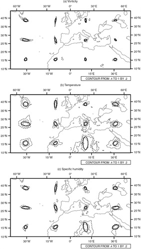
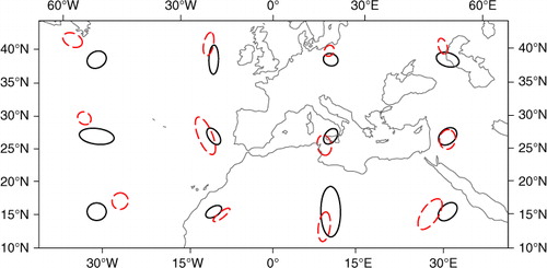
The length scale and anisotropy diagnostics introduced by Pereira and Berre (2006), Michel (2013b), and Ménétrier et al. (2014) are local, e.g. they are related to the local behaviour of the correlation functions. Figure 3 shows a simplified representation of correlation function with elliptic shapes. Ellipses have their major axes in the direction of the main eigenvectors (associated with the smallest eigenvalues λ₁). Ratios between minor and major axe lengths equal . The simplified visualisation of the correlation function with ellipses is compared with raw correlation functions at 3×4 observation points. Anisotropy, length scales and orientation of each ellipse shows good similarities with the raw correlation function. This indicates that for the global model ARPEGE, these low–cost diagnostics are actually rather good representation of the correlation functions, and that they can be used for our purpose of comparing the effect of deformations on the correlation structure. In addition, a total length scale can be computed. Similarly to Ménétrier et al. (2014), it is defined here as the geometric mean .

Fig. 3 Superposition of the correlation function (contoured at 0.4, 0.6, and 0.8 in dashed thin lines) with the ellipses determined from the inertia matrix (solid bold lines). Correlations are computed at level 60 (≈900 hPa) for (a) vorticity, (b) temperature, and (c) specific humidity. For divergence the superposition is very similar to the vorticity one but with smaller correlation lengths (not shown).

3.5. Invertibility of the deformation

The framework requires the estimated deformation to be invertible. This is not ensured by construction, e.g. both the ST and the GT can be singular. The choice made in this study is to enforce invertibility through spatial smoothing.

First estimations of the ST showed that the deformations are non-invertible only at a few grid points. This particularly affects the specific humidity error fields. To avoid this issue, the smoothing step [eq. (22) of Clerc and Mallat (2002)] initially used to increase the robustness of the statistical estimation is reinforced. Indeed large filter lengths L are chosen to smooth enough fields to avoid change of sign of det(J _d ). Too large values of the filter lengths would lose signal in the estimated deformation, such that a compromise should be done. Michel (2013a) averages the spatial derivatives in wavelet space with a length of L=8 grid points. In our case this was found to be insufficient to ensure invertibility.

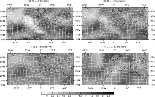
Figure 4 shows det(J _d ) values and the deformed grid associated to d ⁻¹ for three values of filter length L=8, L=12, and L=20 grid points. With a similar set up of L=8 grid points as Michel (2013a), non-invertible areas remain. For L=20 the loss of resolution may be too high. A filter length L=12 grid points for every variable and every level is the lower value that avoids the null or negative values of det(J _d ) in the tropospheric levels. For the rest of this paper L=12 grid points will be chosen as the filter length for all four variables and all levels.

Fig. 4 Grid-lines bending of a regular grid induced by the deformation d. The resulting deformed grid represents in transformed space the contour of the physical space coordinate. Deformation presented in (a), (b), and (c) are objectively estimated with the ST. Different values of L are presented: (a) L=8 grid points, (b) L=12 grid points, and (c) L=20 grid points. Backgrounds of each panel represent values of det(J _d ) the Jacobian determinant of the deformation at each grid point. Changing sign areas (noted with dashed thin lines) for det(J _d) induced a crossing of deformed grid-lines causing non-invertibility. Those results are for the specific humidity at level 35 (≈300 hPa). (d) The corresponding grid-lines bending and the Jacobian determinant of the deformation estimated with the GT, with L=12 grid points.

In stratospheric levels, deformations have been found to remain non invertible near the domain boundaries despite this tuning of the filter length L. This was traced back to the way the wavelet coefficients are computed using fast Fourier transforms. Improvement was achieved with a better biperiodisation approach. The chosen solution was to periodise error fields with a periodic cubic splines and then to zero out the wavelet coefficients that are located in the cone of influence (Mallat, 2008) of the boundaries.

The deformations estimated with the GT are also non-invertible (e.g. crossing lines in Fig. 1 over the North part of the cold front). To ensure its invertibility, a similar smoothing step has been applied. The same filter length L=12 grid points is used for all four variables and vertical levels. This is made to keep the same setup for ST and GT.

As mentioned in the introduction, this study is not dealing with the balance relationships. The ARPEGE data assimilation scheme uses the formulation of Derber and Bouttier (1999). All variables are approximately uncorrelated by using the balance operator. This debalancing procedure removes the balanced part of the temperature and of the divergence. Vorticity and specific humidity are left unaltered.

4. Results

From the 90 member ensemble, the anisotropy index O and the total length scales L _t are computed for every level and every (unbalanced) variable, both in physical (deformed) and computational (inverse) spaces.

4.1. Anisotropy

Background error correlations are more isotropic when the anisotropy index O is lower. In order to present a synthetic view of the results, the anisotropy index has been averaged over the horizontal. The vertical profiles are presented in Fig. 5. On average, the error correlations show pronounced anisotropy in the lower stratosphere (between 100 and 200 hPa). They are more isotropic at the top of the boundary layer (between 850 and 900 hPa) than at the surface for all variables but vorticity. The surface and in particular the orography is indeed likely to have an influence on the anisotropy of the background errors.

Fig. 5 Vertical profiles of the anisotropy O, for (a) vorticity, (b) divergence, (c) temperature, and (d) specific humidity, for the ensemble in physical space (solid lines) and in computational space after applying the inverse of the deformation estimated with the ST (dotted lines) and with the GT (dashed lines). O is averaged over the whole domain (except near boundary points) on the 7th of November 2011 at 12UTC.

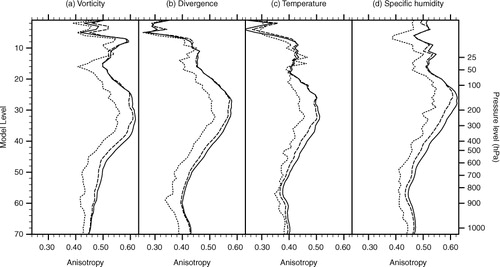
Figure 5 shows that on average both the GT and the ST have a positive impact at least in the troposphere (up to 150 hPa), in the sense that the mean anisotropy is lower in inverse space than in physical (deformed) space. The strongest improvement for both algorithms is located in the higher troposphere (around level 35, approximately 300 hPa). According to the anisotropy vertical profile of the raw ensemble, this layer is also the place where the anisotropy itself is largest. The decrease of the mean anisotropy is systematically higher for the ST than for the GT (apart from model level 15 for temperature). For temperature, using the ST, the anisotropy O at level 35 is decreasing from 0.5 to 0.42 (equivalent to a 14% reduction of length of the major axe of an ellipse), meanwhile with the GT O is only decreasing to 0.46 (equivalent to a 7% reduction of the length of the major axe of an ellipse).

The efficiency of the GT in diminishing the mean anisotropy is dependent on the vertical level. Close to the surface and in the stratosphere above level 25 (=100 hPa) the GT has a neutral impact. In the troposphere between level 55 (≈800 hPa) and level 30 (≈200 hPa), it clearly has a greater efficiency. Maybe it has a connection with the fact that the QG assumptions (R _O ≪1, with R _O the Rossby number) may be more valid at those levels than at the surface or the tropopause. In agreement with Semple (2001), this study highlights that the use of the GT in modelling background error correlations may be physically appealing in frontal areas of extratropical cyclones. As measured by our metric, it is however less efficient than the ST.

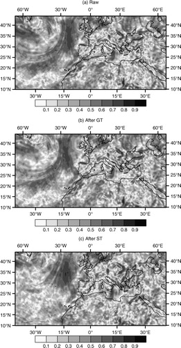
According to the Fig. 5, the ST and GT (in smaller manner) are on average decreasing the anisotropy over the domain. But this result does not give information on the local behaviour. In Fig. 6, anisotropy maps of the raw ensemble are presented and the undeformed ensemble in transformed space after the ST and the GT. The average decrease with GT and ST is confirmed especially around the frontal area. While the cold front structure is still visible after the GT, for the ST, it shows a clear decrease of O on the bottom left part of the domain with an almost complete isotropisation of the south part of the cold front. Elsewhere in the domain, the anisotropy is also decreasing but in a smaller way.

Fig. 6 Maps of anisotropy for (a) the raw ensemble, (b) the ensemble undeformed with the GT, and (c) the ensemble undeformed with the ST. The variable is temperature on the 7th of November 2011 at 12UTC at level 60 (≈900 hPa). Near boundaries points are also avoided. One notices that for the raw ensemble the background coast lines are exact. But for the two other panels, since the ensemble has been undeformed, they are not corresponding to the foreground and are just drawn to simplify the recognition of the features with the top panel.

4.2. Heterogeneity

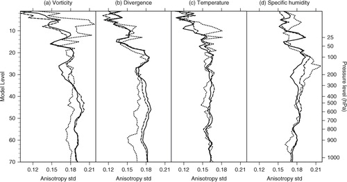
If the correlations were homogeneous over the domain, the standard deviations of the oblateness index and of the total length scale would be reduced to zero. Figure 7 presents the standard deviation of the oblateness index O over the domain. For levels 35–65 (from ≈250 hPa to the boundary layer), the standard deviation is globally diminished after the ST and also after the GT, yet in a smaller manner.

Fig. 7 Vertical profiles of the standard deviation of anisotropy O, for (a) vorticity, (b) divergence, (c) temperature, and (d) specific humidity, for the ensemble in physical space (solid lines) and in transformed space after applying the inverse of the deformation estimated with the ST (dotted lines), or after the GT (dashed lines). Results are averaged over the whole domain (except near boundary points) on the 7th of November 2011 at 12UTC for ARPEGE model.

Figure 8 represents the standard deviation of the total length scale for each vertical level and variable. As regards the ST, the undeformed ensemble has lower total length scale standard deviations as well as the anisotropy standard deviations (Fig. 7) from the surface to the mid–troposphere. In this case this diminution is the highest for temperature at the surface, with a decrease of the standard deviation from 72 to 54 km. This is illustrated in Fig. 9 with the simplified representation with ellipses of the correlations in physical space and in transformed space after the ST. Large total length scales of both the South–East and the West of the domain are clearly diminished by the ST, giving overall less variation of the length scales over the domain. Despite an increase of the ellipses size along the frontal area, the ellipses size are more homogeneous over the domain for the ensemble in computational (inverse) space.

Fig. 8 Vertical profile of standard deviation of total length scale L _t , for (a) vorticity, (b) divergence, (c) temperature, and (d) specific humidity, for the ensemble in physical space (solid line) and in transformed space after applying the inverse of the deformation estimated with the ST (dotted line), or after the GT (dashed line). Near boundary points were also neglected. Stratospheric model levels from 1 to 19 are not represented.

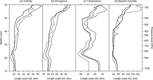
Fig. 9 Superposition of simplified elliptic visualisation of the correlation of the raw ensemble (solid lines) and of the ensemble in transformed space after ST (dashed lines). Correlation tensors are computed at level 60 (≈900 hPa) for temperature. For each position (4×5), ellipses for the raw ensemble and for the ensemble in transformed space are not superposed since error fields have been displaced by d ⁻¹.

At higher levels (above 600 hPa), the standard deviation of the total length scale is increased by the ST for every variable (Fig. 8); therefore, the improvement brought by the ST on homogeneity is limited to lower tropospheric levels (under 700 hPa). Elsewhere, the decrease of anisotropy and its variations are accomplished at the detriment of the heterogeneity of the total length scale.

The GT does not really affect the standard deviation of the anisotropy (Fig. 7). However, the standard deviation of the total length scale increases at all vertical levels for all variables but humidity (Fig. 8). This shows that the GT does introduce some spurious inhomogeneities in the modelled correlations in a systematic way (e.g. for all variables and vertical levels).

4.3. Diagnostics in the stratosphere

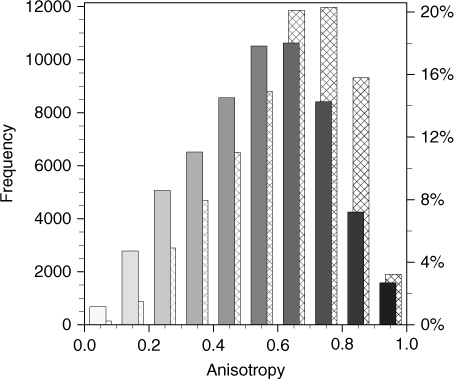
In stratospheric levels (levels≤25), the decrease of standard deviation of the anisotropy index is no longer systematic with the ST, with a large increase, for example at level 25 (≈150 hPa) for the specific humidity variable. Moreover, the total length scale standard deviation is increasing for most levels and variables (not shown). A different way of looking at these results is proposed in Fig. 10. The mean anisotropy is clearly decreasing, but the standard deviation does not. Yet, the distribution of anisotropies over the domain appears better in computational space than in physical space, with less values of strong anisotropies.

Fig. 10 Distribution histogram of anisotropy O over the domain for the raw ensemble (hatched bars, background) and the ensemble undeformed with the ST (filled bars, foreground), for specific humidity, on the 7th of November 2011 at 12UTC for ARPEGE model at the stratospheric level 25 (≈150 hPa).

It is clear that applying the inverse deformation is not removing all the anisotropy or the heterogeneity. Perhaps using the deformation approach together with another heterogeneous modelling approach could be useful [for instance the wavelet approach from Deckmyn and Berre (2005) or the inhomogeneous recursive filters from Purser et al. (2003b)]. Progress could be expected also by going to a fully three-dimensional computation of the statistical deformation.

As regards the GT, for every variable and every level, the standard deviation of the total length scale is increasing except for a few levels for the specific humidity. This makes this transform probably less useful than the ST for the modelling of background error correlations.

4.4. Comparing the deformations between variables

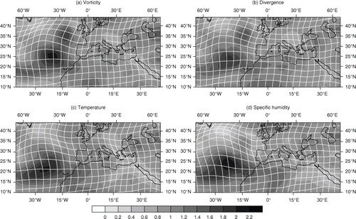
The deformation acts on unbalanced variables to represent the anisotropies and heterogeneities of their horizontal correlations. Another possibility is to use the same deformation for all variables. This may allow commuting the spatial deformation with the balance transform. We have found close similarities between the statistical deformations estimated for the different variables. In Fig. 11, the Jacobian of the deformation for all four variables studied is represented. The features modelled by the deformation are located at the same places and almost have the same shape. Only the amplitude is variable. Despite using unbalanced (i.e. mostly uncorrelated) variables, the algorithm is detecting the same convergent and divergent areas. This result would support the fact that the anisotropy of structure functions are similar enough such that the same deformation could be used for all variables. This conclusion has however to be mitigated for high stratospheric levels and surface level where the deformation varies more between each unbalanced variable (not shown).

Fig. 11 Jacobian determinant of the deformation (grey shades) and the regular grid deformed by the deformation d (white lines, as Fig. 4) estimated by ST for (a) vorticity, (b) divergence, (c) temperature, and (d) specific humidity, at level 60 (≈900 hPa).

5. Conclusions

This study compares two deformations (coordinate changes) proposed for the modelling of the background error correlations in meteorological data assimilation. This comparison uses a large ensemble of data assimilations to make this comparison on a case study. The accuracy of the deformation and so the quality of the correlation function modelling is quantified by calculating the decrease of the anisotropy and heterogeneity of correlations between the raw ensemble of forecasts with its undeformed representation in transformed space.

The ST is shown to systematically decrease the averaged anisotropy for every level and every control variable. The biggest improvements of the algorithm are located in the higher troposphere. In contrast, the improvements brought by the GT are lower and limited to the frontal area of an extra-tropical cyclone. Overall, both algorithms are diminishing the heterogeneity of the anisotropy. The ST is decreasing the heterogeneity of the total length scale in the lower half of the troposphere, but increasing it at higher levels. It may be that there is a ‘competition’ into getting more isotropic correlation functions versus more homogeneous ones. The GT is increasing the heterogeneity for every level and variable.

It is possible that the deformed, flow-dependent horizontal correlation may interact with the multivariate aspects of the parameter transform. In spite of the fact that the variables were previously unbalanced by the parameter transform, the statistical deformations estimated for all variables are very similar. Only the amplitude of the deformation varies between variables. This would support the idea of estimating a single deformation for all variables, and possibly to try to commute the application of the deformation operator with the multivariate transform. This would mean that the total and balanced increment would then be stretched by the grid change. This might lower this interaction effect but clearly this has to be studied in much more detail.

In this study, the statistical deformation is designed to model the anisotropy and heterogeneity of correlations over the horizontal domain. The extension to three dimensions is possible when original correlations are also stationary over the vertical or at least separable. This is not the case of the background error model used here, which makes the problem more complex. However, we expect that the method could be applied to localisation functions rather than correlations. Most localisation schemes are indeed using separable formulations. The spatial deformations estimated from the ST could therefore be used in ensemble assimilation approaches for building heterogeneous and anisotropic localisations, as illustrated in Michel (2013a). This will be the topic of future studies.

6. Acknowledgements

This study benefited from the support of the MISTRAL-HYMEX research program and from the RTRA STAE foundation within the framework of the FILAOS project. The authors thank Benjamin Ménétrier for his scientific advice. The careful readings of Thibaut Montmerle, Tom Auligné and Philippe Arbogast also proved very useful to improve the manuscript.

Notes

¹ Action de Recherche Petite Échelle Grande Échelle (Pailleux et al., 2000).

² Assimilation d'Ensemble ARPEGE.

References

- Bannister R. N . A review of forecast error covariance statistics in atmospheric variational data assimilation. II: modelling the forecast error covariance statistics. Q. J. Roy. Meteorol. Soc. 2008; 134(637): 1971–1996.
- Benjamin S. G . An isentropic meso α-scale analysis system and its sensitivity to aircraft and surface observations. Mon. Weather Rev. 1989; 117(7): 1586–1603.
- Berre L . Estimation of synoptic and mesoscale forecast error covariances in a limited-area model. Mon. Weather Rev. 2000; 128: 644–667.
- Berre L. , Desroziers G . Filtering of background error variances and correlations by local spatial averaging: a review. Mon. Weather Rev. 2010; 138(10): 3693–3720.
- Bouttier F . The dynamics of error covariances in a barotropic model. Tellus A. 1993; 45(5): 408–423.
- Bouttier F . A dynamical estimation of forecast error covariances in an assimilation system. Mon. Weather Rev. 1994; 122: 2376–2390.
- Chaboureau J.-P. , Nuissier O. , Claud C . Verification of ensemble forecasts of Mediterranean high-impact weather events against satellite observations. Nat. Hazards Earth Syst. Sci. 2012; 12(8): 2449–2462.
- Clerc M. , Mallat S . The texture gradient equation for recovering shape from texture. IEEE Trans. Pattern Anal. Mach. Intell. 2002; 24(4): 536–549.
- Courtier P. , Andersson E. , Heckley W. , Vasiljevic D. , Hamrud M. , co-authors . The ECMWF implementation of three-dimensional variational assimilation (3D-Var). I: formulation. Q. J. Roy. Meteorol. Soc. 1998; 124(550): 1783–1807.
- Deckmyn A. , Berre L . A wavelet approach to representing background error covariances in a limited-area model. Mon. Weather Rev. 2005; 133: 1279–1294.
- Derber J. , Bouttier F . A reformulation of the background error covariance in the ECMWF global data assimilation system. Tellus A. 1999; 51(2): 195–221.
- Desroziers G . A coordinate change for data assimilation in spherical geometry of frontal structures. Mon. Weather Rev. 1997; 125(11): 3030–3038.
- Ducrocq V. , Belamari S. , Boudevillain B. , Bousquet O. , Cocquerez P. , co-authors . HyMeX, les campagnes de mesures: focus sur les événements extrêmes en Méditerranée. La Météorologie. 2013; 80: 37–47.
- Fisher M . Generalized frames on the sphere, with application to the background error covariance modelling. Proceedings of ECMWF Seminar on Developments in Numerical Methods for Atmospheric and Ocean Modelling. 2004; UK: Reading. 87–101.
- Hamill T. M. , Snyder C. , Morss R. E . Analysis-error statistics of a quasi geostrophic model using three-dimensional variational assimilation. Mon. Weather Rev. 2002; 130(11): 2777–2790.
- Hoskins B. J . The geostrophic momentum approximation and the semi-geostrophic equations. J. Atmos. Sci. 1975; 32(2): 233–242.
- Hoskins B. J. , Bretherton F. P . Atmospheric frontogenesis models: mathematical formulation and solution. J. Atmos. Sci. 1972; 29(1): 11–37.
- Mallat S . A Wavelet Tour of Signal Processing: The Sparse Way. 2008; Burlington, MA: Academic Press, Elsevier.
- Ménétrier B. , Montmerle T. , Berre L. , Michel Y . Estimation and diagnosis of heterogeneous flow-dependent background error covariances at convective scale using either large or small ensembles. Q. J. Roy. Meteorol. Soc. 2014; 140: 2050–2061.
- Michel Y . Estimating deformations of random processes for correlation modelling in a limited area model. Q. J. Roy. Meteorol. Soc. 2013a; 139: 534–547.
- Michel Y . Estimating deformations of random processes for correlation modelling: methodology and the one-dimensional case. Q. J. Roy. Meteorol. Soc. 2013b; 139: 771–783.
- Nordeng T. E . A Simple and Efficient Method to Obtain Flow Dependent Structure Functions for Objective Analysis of Weather Elements. 1998. HIRLAM4, Technical Report, no. 36, August 1998, c/o Met Éireann, Glasnevin Hill, Dublin 9, Ireland.
- Pailleux J. , Geleyn J.-F. , Legrand E . La prévision numérique du temps avec les modèles ARPÈGE et ALADIN-Bilan et perspectives. La Météorologie. 2000; 30: 32–60.
- Pereira M. B. , Berre L . The use of an ensemble approach to study the background error covariances in a global NWP model. Mon. Weather Rev. 2006; 134(9): 2466–2489.
- Perrin O. , Senoussi R . Reducing non-stationary stochastic processes to stationarity by a time deformation. Stat. Probab. Lett. 1999; 43: 393–397.
- Purser R. J. , Wu W.-S. , Parrish D. F. , Roberts N. M . Numerical aspects of the application of recursive filters to variational statistical analysis. Part I: spatially homogeneous and isotropic Gaussian covariances. Mon. Weather Rev. 2003a; 131(8): 1524–1535.
- Purser R. J. , Wu W.-S. , Parrish D. F. , Roberts N. M . Numerical aspects of the application of recursive filters to variational statistical analysis. Part II: spatially inhomogeneous and anisotropic general covariances. Mon. Weather Rev. 2003b; 131(8): 1536–1548.
- Raynaud L. , Berre L. , Desroziers G . An extended specification of flow-dependent background error variances in the Météo-France global 4D-Var system. Q. J. Roy. Meteorol. Soc. 2011; 137(656): 607–619.
- Raynaud L. , Berre L. , Desroziers G . Accounting for model error in the Météo-France ensemble data assimilation system. Q. J. Roy. Meteorol. Soc. 2012; 138(662): 249–262.
- Semple A . A Meteorological Assessment of the Geostrophic Co-ordinate Transform and Error Breeding System When used in 3D Variational Data Assimilation. 2001; NWP Tech Rep, UK. 357.
- Snyder C. , Hamill T. M. , Trier S. B . Linear evolution of error covariances in a quasigeostrophic model. Mon. Weather Rev. 2003; 131(1): 189–205.
- Varella H. , Berre L. , Desroziers G . Diagnostic and impact studies of a wavelet formulation of background-error correlations in a global model. Q. J. Roy. Meteorol. Soc. 2011; 137(658): 1369–1379.