Arctic Ocean freshwater composition, pathways and transformations from a passive tracer simulation

Abstract

Freshwater (FW) induced transformations in the upper Arctic Ocean were studied using a coupled regional sea ice-ocean model driven by winds and thermodynamic forcing from a reanalysis of data during the period 1948–2011, focusing on the mean state during 1968–2011. Using passive tracers to mark a number of FW sources and sinks, their mean composition, pathways and export were examined. The distribution of the simulated FW height reproduced the known features of the Arctic Ocean and volume-integrated FW content matched climatological estimates reasonably well. Input from Eurasian rivers and extraction by sea-ice formation dominate the composition of the Arctic FW content whilst Pacific water increases in importance in the Canadian Basin. Though pathways generally agreed with previous studies the locus of the Eurasian runoff shelf-basin transport centred at the Alpha-Mendeleyev ridge, shifting the Pacific–Atlantic front eastwards. A strong coupling between tracers representing Eurasian runoff and sea-ice formation showed how water modified on the shelf spreads across the Arctic and mainly exits through the Fram Strait. Transformation to salinity dependent coordinates showed how Atlantic water is modified by both low-salinity shelf and Pacific waters in an estuary-like overturning producing water masses of intermediate salinity that are exported to the Nordic Seas. A total halocline renewal rate of 1.0 Sv, including both shelf-basin exchange and cross-isohaline flux, was estimated from the transports: both components were of equal magnitude. The model's halocline shelf-basin exchange is dominated by runoff and sea-ice processes at the western shelves (the Barents and Kara seas) and Pacific water at the eastern shelves (the Laptev, East Siberian and Chukchi seas).

• Arctic Ocean
• freshwater
• pathways
• water mass transformation
• passive tracers

1. Introduction

One of the key features of the Arctic Ocean is the stable stratification due to the sharp salinity gradient in the upper ocean. This effectively inhibits the heat stored in the warmer Atlantic water (AW) layer from penetrating upwards and potentially melting the sea ice (e.g. Martinson and Steele, 2001). The Arctic Ocean receives large amounts of freshwater (FW) compared to its relatively small ocean volume (McClelland et al., 2011). The largest FW source is continental runoff from Eurasian and American rivers. A FW budget using the commonly cited reference salinity 34.8 (Serreze et al., 2006) places the low-salinity Pacific water (PW) as the next largest source: other contributions are from net precipitation over the open ocean, which is mainly positive, and seasonal sea-ice melt.

Most parts of the FW are stored in the polar mixed layer (PML), which usually penetrates to depths of 30–50 m. The PML is strongly affected by the variations in the large-scale atmospheric forcing typically alternating between a mode of strong anti-cyclonic circulation centred over the Canada Basin and a mode with weaker anti-cyclonic circulation and stronger cyclonic circulation primarily over the shelf seas and the Eurasian side (Hunkins and Whitehead, 1992; Proshutinsky and Johnson, 1997). In the anti-cyclonic regime Ekman convergence collects FW from the periphery and accumulates it in the Beaufort Gyre, while the cyclonic regime releases FW which can then be transported towards the main gates in the Canadian Arctic Archipelago (CAA) (Proshutinsky et al., 2002, 2009). Moreover, FW from the Eurasian rivers also has a strong coupling to the large-scale circulation. In the cyclonic mode, runoff-diluted waters tend to stay on the shelf and flow further east and accumulate in the Laptev and East Siberian seas. In contrast, when atmospheric vorticity is anti-cyclonic over the shelf, runoff-diluted waters migrate northwards towards the central Arctic Ocean (e.g. Newton et al., 2006; Dmitrenko et al., 2008). In recent years, an increase of FW and wind stress over the Canada Basin has been observed (Proshutinsky et al., 2009; Rabe et al., 2011; Giles et al., 2012). However, the circulation has not strictly been in the anti-cyclonic regime during the recent years suggesting that there is more complexity in the system than can be described by changes in large-scale wind forcing and the Ekman convergence. Morison et al. (2012) also argue that a more cyclonic circulation would lead to more Eurasian runoff contributing to the observed freshening in the Canada Basin. Furthermore, hydrographic and tracer observations show that the water masses below the PML have a delayed (Morison et al., 2006) or decoupled response (Alkire et al., 2007) to the large-scale atmospheric regime shifts.

The PML is distinctively different from the warmer and saltier AW and in between the layers a halocline exists that over most central regions coincides with near-freezing temperatures and is hence called a ‘cold’ halocline. The high salinities and near-freezing temperature of the halocline waters imply that it cannot simply be a product of mixing between the PML and AW; other processes must influence the formation of these water masses. Several different mechanisms have been proposed to explain how water masses with the right characteristics can be produced. Basically they fall into two categories: (1) water masses that have been transformed on the shelf and are transported towards the central regions (Coachman and Barnes, 1962; Aagaard et al., 1981; Steele et al., 1995); or (2) a process that occurs in the interior Arctic Ocean where the upper part of the inflowing AW is transformed by winter convection and summertime melting (Rudels et al., 1996, 2004). The composition of the halocline is also highly dependent on the location. In the Canada Basin PW dominates the upper halocline, whereas shelf-modified waters are more abundant in the Makarov and Amundsen basins. The lower halocline is mostly produced from AW in the Nansen Basin and Barents Sea and circulates cyclonically around the central basins (Rudels et al., 2004). The cold halocline is by no means a stationary feature and has been observed to retreat and advance over the Amundsen Basin in response to changing pathways of the low-salinity surface water, caused by shifts in atmospheric conditions (e.g. Steele and Boyd, 1998; Björk et al., 2002).

The FW balance of the Arctic Ocean is clearly complex. However, one can use a much simpler approach and consider the Arctic as a two-layer system made up of a fresh active surface layer and a stagnant lower layer with AW properties (e.g. Stigebrandt, 1981). In such a system the Arctic resembles an estuary where the main inflow component (AW) is transformed into a water mass with lower salinity due to interactions with the Pacific and/or fresh water sources. Rudels (2010) showed that such a simple two-layer model subjected to geostrophically controlled exchange flows gives a realistic estimate of the horizontally averaged FW height in the Arctic Ocean.

However, the FW height has strong gradients within the Arctic Ocean and it is thus important to understand how and where the different internal FW sources interact with the inflowing water from the Atlantic and Pacific oceans. To this end, the Arctic Ocean has been extensively studied using geochemical tracer observations (e.g. Östlund and Hut, 1984; Schlosser et al., 1994; Bauch et al., 1995; Jones et al., 2008), providing information about the composition and residence times for many of the FW sources. But observations are sparse in time and space so many modelling studies have been undertaken to complement the observations. Previous modelling studies have investigated the role of both runoff and/or PW in the Arctic Ocean using mainly passive tracers (Harms et al., 2000; Maslowski et al., 2000; Karcher and Oberhuber, 2002; Prange, 2003; Newton et al., 2008; Condron et al., 2009; Jahn et al., 2010). The studies have primarily focused on: the pathways of the Siberian rivers – spreading eastwards – and their sensitivity to atmospheric circulation, the export of water of Pacific and Eurasian shelf origin on both sides of Greenland, and pathways of AW. Only one study, using the Community Climate System Model version 3 (CCSM3) – a coarse-resolution coupled climate model, has also incorporated tracers representing sea-ice melting and formation processes (Jahn et al., 2010).

In this paper, we apply a regional sea ice-ocean model forced by data from an atmospheric reanalysis to study how FW sources transform the upper Arctic Ocean. The approach is similar to that of Jahn et al. (2010). We include a number of passive tracers that represent the major FW sources, however, we use a forced sea ice-ocean model which is not sensitive to inherent coupling biases, e.g. northward shift of the Beaufort high pressure (DeWeaver and Bitz, 2006). Other notable differences between our model and their CCSM3 configuration are: a horizontal resolution of 1/4° vs. 1°, 2 channels in the CAA vs. 1, and an open coastal connection between the Laptev and East Siberian seas. These bathymetric features are potentially important for the spreading of FW. From the passive tracers we examine the composition of FW in the central Arctic Ocean and infer pathways of how low saline water is transported through the system. To further understand how source waters form the upper fresh layer we study the water mass transformations and exchanges in salinity-dependent coordinates where particular focus is paid to the Arctic halocline and how it is ventilated. The results are also, in some cases, compared to estimates based on simplified theoretical models to further aid their interpretation.

The article is organised as follows. In Section 2, we present the model experiment as well as theory of how water mass transformation can be studied in salinity coordinates. In Section 3, we present and discuss our main results. In the final section, we summarise and conclude the main findings of our work.

2. Methods

2.1. Ocean circulation model

The model used in this study is the Rossby Centre Ocean model (RCO), applied to the Arctic Ocean. RCO is a Bryan–Cox–Semtner primitive equation model with a free surface and open boundary conditions (Webb et al., 1997). The model domain covers the Arctic Ocean, the Bering Sea, and the North Atlantic to roughly 50°N. It has a horizontal resolution of 1/4° (28 km) and 59 unevenly spaced vertical levels using z-coordinates. In the Arctic Ocean the Rossby radius is of the order of 5–15 km and the model is thus not resolving meso-scale eddies. The vertical mixing is calculated from the KPP scheme by Large et al. (1994).

In the North Atlantic Ocean, open boundary conditions for temperature, salinity and tracers are implemented following Stevens (1991). For temperature and salinity, inflows are nudged towards monthly data of the Polar Science Center Hydrographic Climatology 3.0 (PHC) (Steele et al., 2001). For sea surface height, prescribed values along the boundary are extracted from a global simulation with the NEMO model (Madec, 2008) [using the ORCA025 configuration and the forcing data set DFS4 (Brodeau et al., 2010)]. In the Bering Sea, the southern boundary is closed. However, to achieve a realistic inflow via the Bering Strait (BeS) a volume flux is prescribed via the surface boundary condition, where a monthly climatology based on Woodgate et al. (2005) is used. FW fluxes are calculated using virtual salt fluxes with a reference salinity of 34.8 and no restoring is applied. Restoring is avoided as it limits our ability to separate the relative contribution of the different FW sources and sinks. The effect of not including a sea surface salinity restoring is further discussed in Section 2.3.

The ocean model is coupled to a multi-category dynamic-thermodynamic sea-ice model that resolves the thickness distribution into seven different ice classes (Mårtensson et al., 2012). The sea-ice rheology is solved using an elastic-viscous-plastic (EVP) model (Hunke and Dukowicz, 1997) and thermodynamics are calculated from a three-layer model (Semtner, 1976). For ice-ocean salinity fluxes sea-ice salinity is assumed to have a constant value of 5.

Using bulk formulae following the protocol of the Arctic Ocean Model Intercomparison Project (AOMIP) air-sea and air-ice fluxes are calculated from 6-hourly surface fields (2m air temperature, 2m specific humidity, 10m winds, sea level pressure, precipitation and total cloudiness) from the NCEP reanalysis project for the period 1948–2011 (Kalnay et al., 1996). River runoff is taken from the AOMIP-protocol, including the 13 major rivers discharging into the Arctic (Prange, 2003). Additional river runoff for the Norwegian coast and the Baltic Sea is also included.

For further details of the RCO model the reader is referred to Meier et al. (2003), Döscher et al. (2010) and Mårtensson et al. (2012).

2.2. Tracer experiment

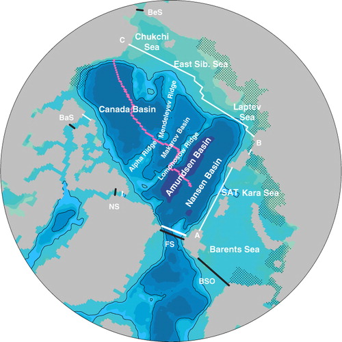
To study how the different FW sources and sinks contribute to the liquid FW composition in the Arctic Ocean, 12 different passive tracers are added to the RCO model. Using a similar approach to that of Jahn et al. (2010), we include the following major components of the FW budget: river runoff, precipitation and evaporation over open ocean areas, sea-ice melt/production and FW inflows. As we are only interested in the FW inside the Arctic Ocean, a region that separates it from the Atlantic and Pacific oceans is defined (see Fig. 1). Inside the region we add, at the surface, five different tracers for river runoff and four tracers for precipitation, evaporation, sea-ice production and melting. On the lateral boundaries, we mark the inflows through the BeS, Barents Sea Opening (BSO) and Fram Strait (FS) with three additional tracers, included as interior source terms. Furthermore, the subdivision of runoff tracers follows the runoff from various catchment areas draining into the Barents, Kara, Laptev, East Siberian seas and the American continent (see Fig. 1 for runoff input patches).

Fig. 1 Map showing the model bathymetry over the Arctic region and geographical locations mentioned in this study: BaS=Barrow Strait, BeS=Bering Strait, BSO=Barents Sea Opening, FS=Fram Strait, NS=Nares Strait, and SAT=St Anna Trough. The bold black lines show the location of the inflow tracers at FS, BSO and BeS. The region within the bold black lines and the Arctic coastline is where the surface tracers for sea-ice melt, sea-ice formation, evaporation and precipitation are injected. The hatched regions show the patches where runoff tracers are injected. The bold white lines are the five boundary segments where transports are calculated in Sections 3.5–3.7: Svalbard–Siberia (A–B), Alaska–Siberia (C–B), BaS, NS and FS. The dotted pink line shows the approximate position of the Beringia transect.

Each tracer is given a concentration relative to the reference salinity S _ref=34.8. We chose this S _ref as it is consistent with the reference salinity used by the virtual salt flux in the model and is commonly used in the literature. However, other choices also occur, e.g. 34.9 or 35.0 and would have worked equally well in this context. Note that, throughout this study we only use 34.8 as reference salinity for FW related quantities. For tracers added at the surface, the concentration c _TR is given a value consistent with the virtual salt flux for the associated FW flux. Thus, tracer representing runoff, precipitation and evaporation have c _TR=1 and sea-ice production/melting tracers a slightly lower value as the virtual salt flux takes into account that some salt is retained/released when sea ice is formed/melted. Inflow tracers on the other hand, are given a c _TR based on the salinity of the inflowing water. To account for recirculation of tracers occurring at the lateral boundaries of the Arctic region (Fig. 1), the sum of recirculating tracers are subtracted from the inflow tracers following Jahn et al. (2010).

As runoff, precipitation, sea-ice melt and Pacific inflows add FW to the Arctic Ocean the corresponding tracers are always positive. Conversely, sea-ice production and evaporation remove FW and tracers are thus always negative. Inflow tracers from the Atlantic Ocean can be both positive and negative depending on the salinity of the inflowing water.

For most of the analysis, we combine some tracers to simplify the interpretation. For instance, all the individual Siberian runoff tracers are combined into a field called Eurasian runoff and occasionally into Eastern and Western contributions. Likewise, we combine precipitation and evaporation tracers into a P–E field and sea-ice melting and formation into a net sea-ice melt (NSIM) tracer.

The time integration of the passive tracers uses the same advective and diffusive operators as salinity in the model. However, as the passive tracer gradient can be different from the salinity gradient – due to different boundary conditions – the diffusive flux could consequently differ. Particularly vertical fluxes can be affected as some of the tracers can have much stronger gradients compared to salinity. This issue will be discussed in Section 3.4.

2.3. Simulation

The simulation starts from an ocean at rest with hydrography from the PHC and sea-ice cover from a previous simulation. We run the model for the period 1948–2011 where we observe that the integrated tracer volumes reach a quasi-steady-state and stabilise after about two decades of integration. We thus consider the first 20 yr as a spin-up and proceed to analyse the remaining 43 yr of the simulation. A spin-up time of 20 yr is longer than the estimated residence time for water masses in the upper Arctic Ocean but below the halocline the spin-up time is expected to be longer. During the first 20 yr, the model FW volume increases with ~17000 km³ over the Arctic Ocean. The following 43-yr period the model exhibits large interannual variability of about ±10000 km³. In the early 1980s and from 2000 there is an increase of FW with a period in the 1990s where FW is lower (not shown). The long-term trend is small (2 km³/yr) and the overall variability is similar to what most models in an intercomparison show (Jahn et al., 2012). The variability of FW, although being an interesting topic, is beyond the scope of the present study and will not be further explored. Instead we will focus on the mean state of the model over the period 1968–2011.

In this study restoring of the salinity field is avoided as it limits the interpretation of the tracers representing FW sources and sinks in the model. This causes some excessive freshening of the upper ocean, partly because the surface boundary condition (virtual salt flux) tends to overestimate the effect of FW where salinity is low (Yin et al., 2010). The resulting model bias is most pronounced on the shelves and in the Eurasian Basin where the influence of the Siberian rivers is most prominent. Another process in the model that affects the FW distribution is vertical mixing. Here we use the KPP scheme with a relatively low background diffusivity (10⁻⁵m²/s), shown by Zhang and Steele (2007) to be a necessity to achieve cyclonic circulation of the AW layer. The low background viscosity and diffusivity together with the excessive amount of freshening yields a sharper stratification, shallower surface mixed layer and a thinner halocline region than observed. Despite these model biases in the upper ocean salinity distribution, we show that the simulation yields valuable qualitative information on the key processes that control the Arctic Ocean FW balance.

2.4. FW and passive tracer quantities

To quantify and compare how the passive tracers contribute to the storage of liquid FW, we calculate a number of FW related quantities. The FW/passive tracer height over a certain depth range is given as,1 where c is either the FW concentration,2 or in the case of the passive tracers the tracer concentration c _TR; z ₁=−256 m and z ₂=0 for the upper ocean or z ₁=z(S=34.3) and z ₂=z(S=31.0) for the halocline inventory. Similarly, the total FW/passive tracer volume over a region A is calculated as,3 and the FW/tracer transport as,4 where s is the length of and u _s the horizontal velocity through a vertical section. Note that negative contributions are allowed in eqs. (1), (3) and (4).

To evaluate the vertical distribution of the FW/passive tracers we calculate a mass-centred depth Z as,5 Z _FW/TR is the first moment of the vertical FW/tracer distribution where FW/tracer storage is weighted with depth – an analogue to centre of mass for FW giving the depth around which the vertical distribution of FW or tracer is centred. Furthermore, if the sum of all tracer distributions has a similar vertical profile as FW then eq. (5) yields information beyond the normal inventory of eq. (1) of the agreement between vertical distributions of FW and passive tracers.

2.5. Water mass transformation in salinity coordinates

Here we present a framework to study exchange and water mass transformation where the basic ideas came from Walin (1977, 1982) and Nilsson et al. (2008). First we consider a region in the Arctic Ocean (see Fig. 1) separating the deeper interior basins from the shelves with a number of vertical sections B. Inside this region we let V(S,t) be the volume of water with salinity less than S bounded by the sea surface and B. Then the conservation of volume for V can be formulated as,6 where M(S,t) is the net transport across a control surface B, G(S,t) the flux across isohalines and E(S,t) the surface flux, all for a salinity value less than S. A net flux is considered positive if it flows in to V(S,t). Further, salt conservation for V can be expressed as,7 where F is the diffusive flux across an isohaline. Differentiating (6) and (7) with respect to S and then multiplying the first with S and subtracting it from the latter, we obtain8

The first term on the right hand side, representing surface processes, will widen the volumetric distribution in S-space and if there is a positive correlation between S and ∂E/∂S also tend to shift the centre of mass of the salinity distribution. The second term, representing mixing, which typically homogenises the distribution in spatial coordinates, will narrow the distribution in S-space. Further, assuming a steady-state and that E is small (6) reduces to,9

Finally, a flux in the salinity range S,S+dS can be evaluated as ∂M/∂SdS, which we will use to evaluate the transport into different salinity layers in Section 3.5.

3. Results and discussion

3.1. FW content and budget in RCO compared to observations

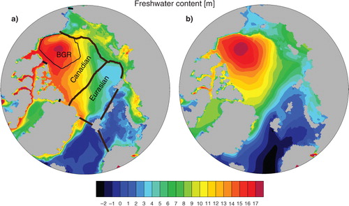
The simulated H _FW is here compared to the PHC to assess how well the model reproduces general features of the climatological FW distribution. However, it should be noted that an exact match is not expected as our simulation covers the period 1968–2011 and the PHC is biased towards observations in the 1970s and 1980s (Jahn et al., 2012). The 1970s and 1980s were dominated by the anti-cyclonic regime (e.g. Proshutinsky et al., 2002) and more recent observations by Rabe et al. (2009) and Proshutinsky et al. (2009) from the 1990s and late 2000s show a shift primarily of the H _FW maximum in the Beaufort Sea and the front between the Canadian and Eurasian side.

Figure 2a shows the mean simulated H _FW of the upper 256m with the characteristic maximum over the Beaufort Gyre Region (BGR) in the Canadian Basin, although it is shifted slightly towards the Canadian coast compared to the PHC (Fig. 2b). The sharp front between the Canadian and Eurasian sector is also somewhat shifted compared to the PHC H _FW and aligned with the Mendeleyev rather than the Lomonosow Ridge. This yields a higher/lower H _FW in the Makarov Basin north of Greenland/East Siberian Sea compared to the climatology. It should be noted that a comparison of only 1970s and 1980s simulated H _FW yields a less pronounced shift (not shown). Within and north of the CAA an excessive accumulation of FW is also evident in the model. Over the Eurasian shelves, especially in the Kara and Laptev seas near the mouths of large rivers, the model tends to overestimate H _FW. This is an effect of the virtual salt flux as mentioned in Section 2.3 and due to a relatively coarse resolution leading to a sluggish shelf circulation (as detailed in Newton et al., 2008). Overall RCO agrees better with more recent observations (Proshutinsky et al., 2009; Rabe et al., 2009) which show a similar shift of the H _FW maximum and front between the Canadian and Eurasian side. A model intercomparsion of several state-of-the-art Arctic Ocean models also yields a similar shift of the mean H _FW (for the period 1990–2002) for most models (Jahn et al., 2012).

Fig. 2 Mean freshwater (FW) height in m integrated over the top 256m for the period 1968–2011 for (a) RCO model and (b) PHC (Polar Science Center Hydrographic Climatology 3.0). The regions marked with black lines in (a) are used to calculate FW/tracer volumes in Fig. 3.

The mean simulated Arctic FW budget in Table 1 is found to be in general agreement with observations, where the major import of FW comes from PW, river runoff and P–E while the main export is liquid FW through the CAA and liquid and solid FW through the FS. However, the inflow from the Bering Sea has a low salinity bias, with a mean salinity of 30.8, averaged over the strait. This leads to a 33% higher FW import that consequently affects the Arctic Ocean FW export. In the CAA, the liquid export is in line with the observed value while the FS export is overestimated by 35%. However, the estimated FS export of 2660 km³/yr from Serreze et al. (2006) is perhaps a lower bound as Rabe et al. (2013) reported a liquid FW export of 3160±730 km³/yr. The solid FW export is somewhat overestimated in the CAA and underestimated at the FS, the latter reducing the total FW export bias somewhat. In the BSO, there is a fresh bias leading to a liquid FW import rather than export while the solid FW transport shows a small export.

Table 1. Comparison of net mean freshwater fluxes from RCO over the period 1968–2011 and observations from compilation by Serreze et al. (2006)

FW fluxes	RCO	Observations
Bering strait liquid	3332	2500
Bering strait solid	112	100
CAA liquid	−3133	−3200
CAA solid	−404	−160
Fram strait liquid	−3598	−2660
Fram strait solid	−1737	−2300
Barents Sea opening liquid	723	−90
Barents Sea opening solid	−151	−
River runoff	3328	3200
P-E	2141	2000
Net	613	−610

All fluxes are in km³/yr calculated with S _ref=34.8.

3.2. Mean FW volume and passive tracer composition

To establish how well the tracers represent the total liquid FW volume and which tracers contribute the most to the FW inventory we examine the volume integrated FW and tracer storages from eq. (3). In Fig. 3 it is seen that the simulated liquid V _FW over the Arctic region is 84.0×10³ km³, 14% higher than the PHC. The Canadian Basin on the other hand, storing more than half of the liquid FW, has a 2% lower content, while the Eurasian Basin has a 9% higher content compared to the PHC. The total V _TR (sum of all tracers in Fig. 3) is 6% higher than the V _FW for the entire Arctic Ocean but for central basins 7–10% lower. Overall, the simulated liquid V _FW and total V _TR are comparable in magnitude for the central Arctic Ocean.

Fig. 3 Mean freshwater/tracer volumes integrated over the top 256m and for different regions (defined in Fig. 2a). The Arctic Ocean region covers both shelves and deeper basins. The Canadian and Eurasian basins are the deeper central parts (depth greeter than 500 m) delineated by the Lomonosov Ridge. Note that the Beaufort Gyre region (BGR) is included in the Canadian Basin.

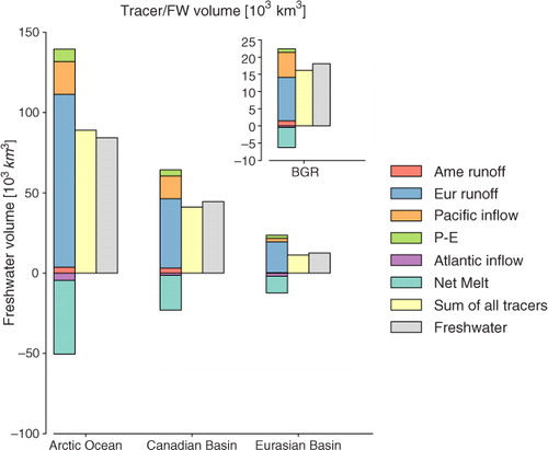
The total V _TR can be divided into the individual tracer components representing the Eurasian and Amerasian runoff, PW, P–E, NSIM, and AW tracer volumes. Note that as the composition is made up of both positive and negative components representing FW anomalies, individual volumes can be higher than the total V _TR. Figure 3 shows that for the entire Arctic Ocean positive, relative contributions are the Eurasian runoff 121%, PW 23%, P–E 9%, and Amerasian runoff 4% and negative contributions are NSIM −46% and AW tracers −5%. As expected, regional differences exist because the locations of the different source regions are different as well as the effect of the Arctic Ocean circulation, which will redistribute the tracers differently. Nevertheless, Fig. 3 shows that the Eurasian runoff and NSIM are always the main positive and negative contributions, respectively. This is most pronounced over the Eurasian Basin, where the PW tracer volume is low, but less so towards the Canadian Basin and the BGR where PW increases. Over a similar region as the BGR, observational estimates yields a FW storage of 15.8±3.5 and 9.8±6 (both in 10³ km³) for meteoric FW and PW, respectively (Yamamoto-Kawai et al., 2008). This is comparable to the total runoff and P–E tracer volume (15.0×10³ km³) and the PW tracer volume (7.0×10³ km³).

As our results show that the Eurasian runoff, PW and NSIM are the dominating tracers, the reminder of the study will mainly focus on these tracers.

3.3. Mean FW pathways and transformations from the passive tracers

To examine how and where FW related processes transform the upper waters of the Arctic Ocean, we use the passive tracers that represent the different FW components. First we analyse the general circulation pattern of the model; then infer pathways based on H _tracer distributions and circulation patterns, and discuss key processes affecting the FW tracers.

3.3.1. Mean circulation.

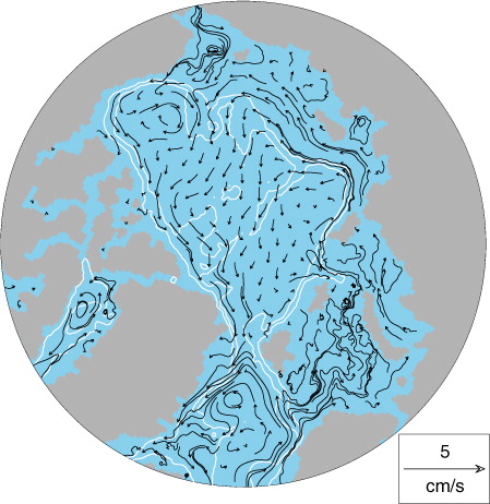
The model's time mean circulation (Fig. 4) is cyclonic over the Eurasian and anti-cyclonic over the Amerasian region. The Transpolar Drift (TPD) is quite broad and aligned with both the Lomonosov Ridge and the Mendeleyev–Alpha Ridge complex, reflecting the shifts in large-scale atmospheric circulation regimes. North of the East Siberian and Laptev seas there is an eastward shelf break current which has a strong barotropic component (not shown) as a result of a large sea surface height gradient, similar to other studies (Maslowski et al., 2000; Newton et al., 2008). Along the shelf break current there is shelf-basin transport into the Nansen, Amundsen and Makarov basins, eventually converging with the TPD. North of the Chukchi Sea the flow from the BeS diverges into either the TPD northwards of the Beaufort Gyre or the coastal current along the Alaskan coast. The latter merges with the current north of the CAA and eventually exits via the FS. At the FS the upper inflow generally follows the same path as the deeper AW layer, steered by topography along the slope of the Nansen Basin with some recirculation into the Barents Sea and St. Anna Trough. The flow over Barents Sea mainly takes two routes: the coastal current flowing eastward towards Kara Sea and the more direct route towards the St. Anna Trough.

Fig. 4 Mean currents (cm/s) averaged over the upper 0–256m overlaid on the 500 and 2000m isobaths (white lines).

3.3.2. Siberian runoff tracers.

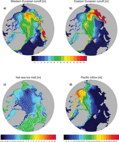
The Siberian runoff tracers (Figs. 5a and 5b) primarily flow eastwards along the shelves and mainly supply the northern Canada, Makarov and Amundsen basins with low-salinity water that is exported through the FS, in agreement with other models (e.g. Harms et al., 2000; Karcher and Oberhuber, 2002; Prange, 2003; Newton et al., 2008; Jahn et al., 2010). For the western Siberian rivers, most of the tracer leaves the inner shelf from the Laptev Sea by either directly entering the Nansen and Amundsen basins or continuing further east along the shelf break later entering the central Arctic Ocean at the Mendeleyev Ridge. Similarly, most of the Eastern Siberian runoff tracer exits the shelf at the Mendeleyev Ridge although some portion of the Laptev Sea runoff migrates northwards and joins the Western Siberian runoff tracer path.

Fig. 5 Mean (1968–2011) passive tracer heights in m integrated over the top 256m and currents averaged over 0–256 m. For (a) the Western Eurasian runoff (the Barents and Kara seas), (b) Eastern Eurasian runoff (the Laptev and East Siberian seas), (c) net sea-ice melt (NSIM) and (d) Pacific water.

Several studies have shown that the shelf-basin exchange is mainly determined by the large-scale wind forcing, where cyclonic/anti-cyclonic circulation tends to decrease/increase the transport off the Laptev Sea (e.g. Dmitrenko et al., 2008; Jahn et al., 2010). A correlation analysis between the Arctic Oscillation (AO) index (or the Vorticity Index) and the Eurasian runoff tracer in our model (not shown) also confirms that more runoff is accumulated in the East Siberian Sea during positive phases, while the Nansen and Amundsen basins receive more runoff during negative phases of the AO.

Once the Eurasian runoff tracers have entered the central basins, the main pathway is along the TPD and 78% is exported through the FS. However, some Eurasian runoff can also be found in the central and northern parts of the BGR, consistent with geochemical observations (Jones and Anderson, 2008; Guay et al., 2009). The remaining export of 22% is equally divided between the Barrow Strait (BaS) and Nares Strait (NS). Jahn et al. (2010) found a higher FS (98%) transport of Eurasian runoff but their model lacks the NS.

3.3.3. Sea-ice tracers.

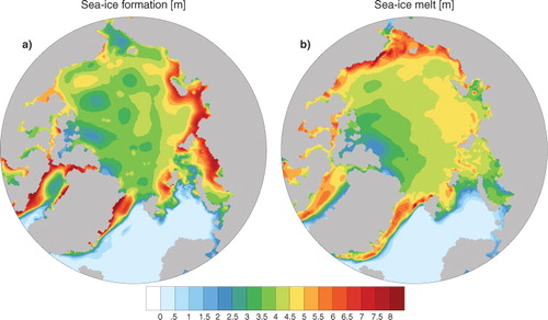
The NSIM tracer, representing the FW input from sea-ice melting and FW removal from sea-ice production, is negative over the upper 256 m, indicating that in the model production exceeds melting (Fig. 5c). Most sea-ice formation is found along the Siberian shelf and around the Arctic islands (Fig. 6a), while the strongest melt signal is seen along the seasonal sea-ice edge in the south-eastern Canada Basin, Chukchi Sea and Eastern East Siberian Sea (Fig. 6b). The production of dense water on the shelf mainly depends on ice formation, water column salinity and depth (Aagaard et al., 1981). This suggests that the western shelves will produce more halocline water than the eastern parts, as the salinity and the ice production in the model are generally higher in those regions.

Fig. 6 In (a) seasonal (October–March) sea-ice formation in m/season averaged over the period 1968–2011 (the sea-ice formation includes frazil and basal ice production) and (b) the seasonal (April–September) sea-ice melt m/season.

Figures 5a–5c show that a strong negative NSIM tracer signal correlates with a high content of the Eurasian runoff tracer in a coherent pattern from the Siberian shelves across the central Arctic Ocean (TPD) towards the FS. A similar pattern with high negative NSIM and low-salinity water, stretching across the central Arctic from the eastern Siberian shelves towards FS, is also found in several studies using geochemical tracers (Yamamoto-Kawai et al., 2005; Bauch et al., 2011; Newton et al., 2013). The strong link between the NSIM and Eurasian runoff tracer, with a temporal correlation of −0.82 (statistically significant at the 95% level), is also seen in the FS, where most of the NSIM tracer (72%) is exported. This is in agreement with geochemical observations by Dodd et al. (2012) showing a strong anti-correlation between meteoric water and NSIM, which they suggest is due to a common source region. Further, they speculate that the signal originates from the shelf seas of the Eastern Arctic which our patterns of NSIM and Eurasian runoff tracers support. The fraction of meteoric to NSIM tracer export through the FS is −2.6 : 1, a somewhat higher meteoric fraction compared to the −2 : 1 that most observations yield (Rabe et al., 2013, and references therein). However, Rabe et al. (2013) also found an increasing fraction of the meteoric FW, with −1.5 : 1.0 in 1998 and −2.5 : 1.0 in 2009.

From Fig. 6, it is evident that there are regions where the melting of sea ice exceeds ice production on an annual basis, seen as regions of slightly negative NSIM tracer in Fig. 5c. These regions broadly reflect areas where warm water from the south enters the Arctic Ocean. In the Atlantic sector, north of Svalbard and in the Barents Sea and the northern Kara Sea, where warm AW melts sea ice and inhibits ice growth, a less negative NSIM is seen. The transformations due to sea-ice melting and formation in these regions are considered to be particularly important for the production of Arctic halocline waters (Steele et al., 1995; Rudels et al., 1996). Likewise, over the Pacific sector the influence of the inflowing warmer PW is seen in the Chukchi Sea and along the Alaskan coast. The sea-ice melt and production tracers have different vertical distributions, with the ice production tracer typically deeper down in the water column. Integrated over the upper 256m this yields a NSIM field that is negative over the Arctic Ocean, on a mean annual basis. However, seasonally as well as close to the surface, the NSIM can of course be positive, which is shown in Section 3.4.

3.3.4. Pacific water tracer.

Figure 5d shows a sharp PW tracer gradient across the Arctic with practically no PW tracer content in the eastern regions. Once the PW tracer leaves the Chukchi Sea, it diverges into two principal branches: the eastern coastal branch following the Alaskan coast and the western TPD branch northwards of the Beaufort Gyre. The main portion of the PW tracer is clearly found in the coastal current and centre of the Beaufort Gyre but the PW inventory also indicates presence of PW north of Greenland and the CAA. The relatively warm PW also contributes to a high melt rate along the coast (Figs. 6b and 9c) and an additional freshening of the upper southern Canada Basin (see also Fig. Fig. 9d).

The partitioning of the simulated PW tracer exchange between the Arctic Ocean and the North Atlantic is BaS (46%), NS (13%) and FS (41%). This is a higher relative export through CAA compared to the 25% found in the study by Jahn et al. (2010), however, they only have one strait representing the CAA throughflow and suggest that their PW export through FS is therefore unrealistically large. The fraction of meteoric to PW to NSIM tracer fractions at the FS is −2.6 : −0.4 : 1.0, comparable to the −2.2 : −0.5 : 1 from observations (Rabe et al., 2013). Dodd et al. (2012) noted a strong variability of the PW fraction in observations covering 1997–2001; a variability that is considered to be forced by shifts in the large-scale circulation regimes (Steele et al., 2004; Alkire et al., 2007).

Previous investigations have shown that the FW and PW distribution over the Canadian Basin is strongly influenced by the variations in large-scale atmospheric circulation (reflected by, e.g. the AO index) and the resulting Ekman transport (e.g. Steele et al., 2004; Condron et al., 2009; Proshutinsky et al., 2009). Indeed a correlation analysis between the AO and the PW inventory (not shown) yields a positive correlation along the North American coast and north of Greenland and a negative correlation in the central Canada Basin. This suggests that PW is released during positive AO and retained during negative AO. Steele et al. (2004) showed that there is a separation with the saltier Bering Sea summer water generally found in the northern Beaufort Gyre and along the TPD whereas the fresher Alaskan coastal waters are generally found in the southern Beaufort Gyre. Possibly the model's low salinity bias in the BeS can influence the separation and spreading of PW in the model towards more PW along the North American coast and less PW in the central Canada Basin and TPD. Another potentially important factor is the role of eddies. Some studies have shown (Pickart, 2004; Spall et al., 2008; Spall, 2013) that there is a vigorous eddy-exchange between the boundary current and the interior basin. The present resolution in our model is not sufficient to resolve meso-scale eddies and could thus influence the PW distribution.

3.3.5. AW tracers.

The AW inflow tracers only give a small negative contribution to the total budget of Fig. 3 as the inventory is calculated relative to a reference salinity that is close to the inflowing salinity at the FS and the BSO. It should be noted though that most of the upper Arctic Ocean consists of AW but this is not clearly reflected by the AW tracers as they are FW anomaly tracers. Nevertheless, the AW tracers can despite their minor contributions to the total FW inventory, yield information about the vertical and horizontal distribution of AW as well as the location of AW transformations.

The flow pattern depicted by the AW tracers in the model agrees broadly with previous modelling studies (Maslowski et al., 2000; Karcher and Oberhuber, 2002) and the observationally inferred paths of the FS and Barents Sea branches of AW (Rudels et al., 2004). We now go on to discuss, based on the different FW tracers, the processes transforming the AW along its path.

In Fig. 7a, it is seen that the FS inflow tracer distribution is negative (i.e. representing a FW deficit) and occupies the western part of the Nansen Basin suggesting a flow along the basin boundary eastwards towards St. Anna Trough with some parts also circulating into the Barents Sea. A weaker negative signal is also seen over most of the Nansen, Amundsen and Makarov basins implying a mean cyclonic circulation over the interior basins. As the relatively warm AW enters the Nansen Basin sea ice melts primarily north of Svalbard (see Fig. 6b) and a signal with less negative NSIM tracer is consequently seen in Fig. 5c. However, Figs. 5a and 5c show that, based on the tracers, meltwater alone cannot contribute to the lower salinities in the upper western Nansen Basin. Instead some FW also originates from the western Eurasian rivers in the model and the ratio of Eurasian runoff to NSIM tracer inventory (upper 256 m) changes from 1.4 : −1 in the eastern Nansen Basin to 2.1 : −1 in the western Nansen Basin. This suggests that a halocline formation, where meltwater is considered to be the only FW source (Rudels et al., 1996), is perhaps not a dominating process in the western Nansen Basin in the model.

Fig. 7 Same as in Fig. 5 but for the Atlantic water (AW) inflow tracers: (a) from the Fram Strait (b) from the Barents Sea Opening.

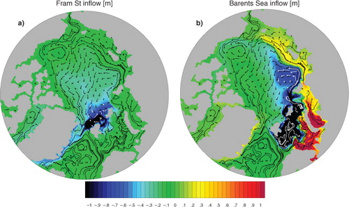
Figure 7b clearly shows how the Barents Sea inflow tracer divides into two branches: the negative branch related to the inflow of water with Atlantic properties and the positive branch representing the Norwegian Coastal Current inflow. The negative tracer branch suggests a north-eastward flow towards St. Anna Trough where it enters the Nansen Basin and circulates along the basin boundary further into the Amundsen and Makarov basins. Again, Fig. 6b shows increased sea-ice melting along the path of the AW inflow tracer with a high seasonal mean melt in the western Barents Sea and the northern Kara Sea. Increased melting in the eastern Nansen and Amundsen basins is also seen. This is due to a thinner ice cover and slightly lower ice concentration in this region, leading to an increased insolation, heating of the mixed layer and subsequent basal ice melt. The absence of runoff and high seasonal melt rate along this path suggests that meltwater is an important FW source for this region in the model, in contrast to the western Nansen Basin. The positive tracer branch in Fig. 7b implies an eastward transport along the Siberian coast and together with Figs. 5a–5c clearly shows how low-salinity shelf water, originating from the Barents Sea, exhibits FW input from rivers and sea-ice meltwater as well as FW extraction from sea-ice production, before it feeds the upper interior Arctic Ocean with low-salinity water.

The pathways inferred from both AW inflow tracers also support the hypothesis proposed by Rudels et al. (2013), that it is primarily the Barents Sea branch that feeds the Arctic halocline, while the FS branch is mostly confined to the Nansen Basin.

3.4. Vertical structure of FW and passive tracers

We now compare the simulated FW and passive tracer distributions with observed hydrography and geochemically inferred FW contributions in a basin-wide transect across the Arctic Ocean taken during August–September 2005; see Fig. 1. For this transect, Jones et al. (2008) calculated end-members for the FW fractions due to meteoric water (river runoff and precipitation), NSIM, and PW using observations of salinity, δ¹⁸ O, alkalinity and nutrient concentrations.

Figures 8 and 9 show the simulated annual-mean FW and passive tracers for the year 2005 in the transect analysed by Jones et al. (2008). (An inspection of monthly model output from the late summer of 2005 (not shown) essentially yields the same hydrographic features, with the exception of a more pronounced sea-ice melt signal near the surface.) The vertically integrated inventories of FW and passive tracers shown in Fig. 8 are qualitatively similar to the observationally based quantities presented by Jones et al. (2008); see their Fig. 4. These similarities include a large gradient in FW height decreasing from ~20 to ~5 m from the Canadian to the Eurasian side; a presence/absence of PW on the Canadian/Eurasian sides explaining most of the FW gradient; a striking anti-correlation between meteoric and NSIM components with extreme values over the TPD region, suggesting an advection from a common source (the Eurasian shelves). The main differences include a too-high meteoric inventory partly compensated by an NSIM that is too low. Additionally, the melt signal is more evident in the observations with positive NSIM over much of the Canada and Makarov basins. This is partly because we use a yearly mean but an examination of monthly values still gives a negative NSIM over the Canadian side in contrast to the observations. It is further seen that the sum of all tracers closely matches the modelled FW inventory over the Nansen and Amundsen basins while there is a mis-match with lower and higher tracer content over the Canada and Makarov basins, respectively.

Fig. 8 Inventories of freshwater (FW), meteoric (runoff and P–E) tracer, Pacific water (PW) tracer, net sea-ice melt (NSIM) tracer and sum of all tracers calculated for the upper 256m from 2005 along the Beringia transect. The location of the transect is shown in Fig. 1.

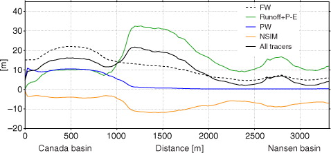
Fig. 9 (a) Mean 2005 freshwater (FW) concentration, (b) meteoric (river runoff and P–E), (c) Pacific water and (d) net sea-ice melt (NSIM) tracer concentrations along the Beringia transect (see Fig. 1 for location). Note that the colour scales are different and that the white contours show the 31, 33, 34, 34.3 isohalines.

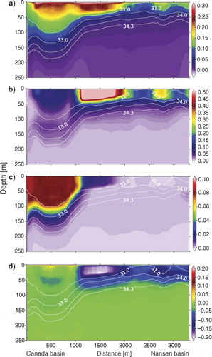
The beginning of the 2000s was a period with persistent anti-cyclonic circulation which resulted in an intensification of the Beaufort Gyre (Proshutinsky et al., 2009). The vertical transects of FW and passive tracers clearly show sign of Ekman pumping with a downward doming over the Canadian Basin (Fig. 9). This is particularly evident in the PW tracer distribution and interestingly the PW and meteoric inventories are of equal magnitude (Fig. 8), in contrast to the mean volume over the full period which suggests more meteoric tracer volume (Fig. 3). Furthermore, there is a pronounced melt signal in the upper Canadian Basin with the NSIM tracer concentration being mostly positive in the upper ~10 m, albeit at a depth the NSIM tracer is negative which explains why the total inventory is negative. A similar vertical distribution is seen in the observations (Jones et al., 2008, their Fig. 3c) although the surface melt signal is stronger leading to a slightly positive NSIM inventory. Most aspects of the geochemical tracer distributions are captured well by the model, with the main differences being: a shift of the Pacific/AW front, a somewhat shallower distribution of all tracers and a fresher Nansen Basin.

To further examine the vertical distribution of FW and passive tracers, we have calculated the mass-centred depths Z associated with these fields; see eq. (5) and Fig. 10. The Ekman convergence on the Canadian side tends to yield distributions that are generally centred deeper in the water column than on the Eurasian side. This feature is particularly pronounced for the observationally based PHC FW field. While the inventories of modelled and climatological FW agree quite well (Fig. 2), the mass-centred depths are distinctly different revealing that the simulated FW distribution is centred much shallower and thus more FW is found higher up in the water column.

Fig. 10 Mass-centred depth distributions Z in m for: (a) PHC (Polar Science Center Hydrographic Climatology 3.0) freshwater (FW), (b) model FW, (c) sum of all passive tracers, (d) Eurasian runoff tracer, (e) Pacific water tracer and (f) net sea-ice melt (NSIM) tracer. Note that regions with depths shallower than the integration depth 256 m, as well as, regions with FW/tracer inventories lower than 0.5 m, have been masked out.

Comparing the FW-based depth distribution (Fig. 10b) with the sum of all tracers (Fig. 10c) shows that the tracers have different depth distributions that do not exactly match the FW-based distribution. Over the Canada Basin and north of the CAA and Greenland, the sum of all tracers is centred slightly shallower, whereas over the Nansen and eastern Amundsen basins the distribution is much shallower than the FW-based depth. Excluding the AW tracers (not shown) yields a better agreement over the Nansen and Amundsen basins implying that it is primarily the AW tracers that shift the vertical distribution in this region. Furthermore, the mass-centred depth distributions of the Eurasian runoff and NSIM tracers shows similar patterns with a ridge along the TPD where tracers are higher up in the water column. The individual Eurasian runoff tracer depth distributions (not shown) also reveal that the Western Eurasian runoff tracers are general centred deeper compared to the Eastern Eurasian runoff tracers. Additionally, it is seen that the PW distribution is flatter and somewhat shallower than the Eurasian runoff tracer along the southern Canada Basin but deeper north of Greenland. The latter is in agreement with observations at the FS showing that meteoric water has a more surface-intensified distribution in the East Greenland Current (Dodd et al., 2012). The fact that the mass centre of the FW associated with the PW is located deeper than that associated with the runoff upstream of the FS has implications for the FW source composition of the flow in the East Greenland Current. Baroclinic transport anomalies, which are more pronounced towards the surface, should give larger fluctuations in the flow of runoff-derived FW than in Pacific-derived FW. Thus, the present model results suggest that in situations with increased baroclinicity of the flow, the transport fraction of runoff-derived FW should increase. This might occur when the large-scale atmospheric circulation changes from an anti-cyclonic towards a cyclonic regime releasing FW from the Canada Basin. However, Jahn et al. (2010) found that changes in the large-scale circulation can also have compensating effects on the total FW export in the FS with PW increasing and Eurasian runoff decreasing as result of such a shift.

3.5. Transport and transformation of water masses in salinity space

To further examine the transport of low and high salinity water masses between the interior Arctic Ocean and its boundaries, we have calculated the cumulative volume transport M(S), which specifies the net inflow of water having a salinity less than S. The net transport M(S) has been calculated separately for the following boundary segments: The FS, Svalbard–Siberia, Alaska–Siberia (including Pacific inflow), NS, and BaS; see Fig. 1. Note that in the FS, we have divided the flow M(S) into one inflow- and one outflow component, as the transport across the strait is inherently bi-directional. For a salinity interval where the derivative of M(S) is positive/negative, water masses with this salinity are transported into/out of the interior Arctic.

Figure 11a shows that the salinity distributions of water that flows across the different sections are quite different. In the FS, where the inflowing AW essentially is unmodified, the inflow occurs in a quite narrow salinity range near 35. In contrast, the FS outflow has a long tail, reaching low salinity followed by a peaked outflow at salinities between about 34.5 and 35. Thus, the upper ocean water masses have been modified by FW input and mixing on its route around the Arctic, manifested by the broad range of salinities in the East Greenland Current. In the Svalbard–Siberia section, the inflow has a narrow peak, representing the weakly modified AW entering mainly through the St. Anna Trough, and a wider tail of lower salinities, representing the Atlantic source waters that have been more strongly blended with FW. There is also a small outflow (into the Barents Sea) detectable as a negative derivative of M(S) in the high end of the salinity. The section between the Alaskan and Siberian coasts is dominated by the Pacific inflow in the range 30–31.5 (this is about 1.0 salinity unit lower than in reality due to the fresh bias in the model's Bering Sea). There is also a small tail due to the water masses that have been diluted by river runoff. The export through the CAA (the BaS and NS) occurs over a wide range of low and intermediate salinities as very little AW is exported through these gates.

Fig. 11 (a) The cumulative transport functions M(S) across the lateral boundaries around the central Arctic Ocean (see Fig. 1) for the period 1968–2011. (b) The red/blue curve is the net cumulative transport across all the boundaries in (a) and the black curve its smoothed gradient. Note that the red/blue regions in (b) correspond to a positive/negative gradient yielding a net inflow/outflow to the Arctic Ocean.

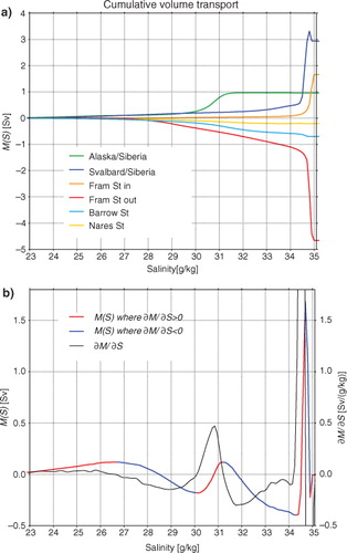
The net cumulative transport M(S) across all the boundary segments highlights the transformation between different salinity classes occurring in the interior Arctic Ocean (see Fig. 11b). As the model simulation is approximately in a steady state, we have M(S) + G(S)=0, implying that the net volume transformation across an isohaline surface G(S) = S∂E/∂S−∂F/∂S can be inferred as −M(S) in Fig. 11b. It is important to note that if no water mass transformation occurred in the interior Arctic Ocean of the model, then G(S) and M(S) would both be identical to zero. This would be the case if the halocline waters were pre-formed in the shelf seas and the Bering Sea and advected through the interior Arctic with no mixing. As shown in Fig. 11b, water mass transformations occur also in the model's interior Arctic Ocean, which has an estuarine character as saline and fresher source waters mix to form outflow waters of intermediate salinities. However, the narrow salinity range of the Pacific inflow and sea-ice formation yield a more complicated structure of M(S) than in a fjord-type estuary, where oceanic water and FW are the only source water masses. Specifically, the net cumulative transport M(S) has here three main inflow contributions in different salinity ranges: low-salinity water masses modified by river runoff, sea-ice melt and growth from the Siberian shelf seas, PW, and AW. The net outflow of water with salinities lower than 34, however, occurs in only two intervals. Thus, in the central Arctic the three net inflow source waters are mixed, creating outflow waters that occupy salinity ranges in between those of the source waters. In the outflow range between 32 and 34.5, there is a net transformation towards lower salinities, i.e. G(S) > 0. This transformation involves AW that is freshened by sea-ice melting and by mixing with fresher waters. For salinities just above 34.5, there is a net transformation toward high salinities that is partly due to net formation of sea ice.

3.6. Halocline renewal in salinity space

Figure 12 summarises the exchange and transformation of water masses in the model's interior Arctic Ocean. Waters in the halocline layer (HL) range are renewed by a net input of 0.5 Sv from cross-isohaline fluxes that mix low-salinity waters with AW and an advection of shelf-modified waters of 0.5 Sv (1 Sv=10⁶m³/s), giving a total renewal rate of 1.0 Sv. Satellite and modelling based estimates of the shelf-modified halocline water are in the range 0.2–1.5 Sv (Björk, 1989; Martin and Cavalieri, 1989; Cavalieri and Martin, 1994; Winsor and Björk, 2000; Nguyen et al., 2012) and the total production rate is assumed to be at least 2.5 Sv (Aagaard et al., 1981). As the halocline is thinner in the model while the residence time is similar to observations an underestimation is expected. Furthermore, Table 2 shows that the shelf-basin volume transport in the PML range is dominated by the Alaska–Siberia section, i.e. the western shelf seas – while the HL range receives a slightly higher input from the Svalbard–Siberia section.

Fig. 12 Sketch showing the exchange between the exterior (the North Atlantic and Eurasian shelf regions) and the interior Arctic Ocean. It also shows exchanges between different layers within the central Arctic Ocean, where the layers are based on salinity ranges: Polar mixed layer (PML) 0 < S<31, halocline layer (HL) 31 < S<34.3 and Atlantic water (AW) layer S>34.3. Note that shelf water consists of both the Pacific water and low-salinity water modified by rivers on the Siberian shelf.

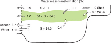
Table 2. Decomposition of water mass into 3 different salinity classes: polar mixed layer (PML) 0–31, halocline layer (HL) 31–34.3 and Atlantic water (AW) layer 34.3–35.5

Alaska/Siberia	Svalbard/Siberia	Fram St in	Fram St out	Barrow St	Nares St	Net
0–31	0.8	0.2	0.0	−0.5	−0.3	−0.1	0.1
31–34.3	0.2	0.3	0.0	−0.6	−0.3	−0.1	−0.5
34.3–35.5	0.0	2.5	1.6	−3.6	−0.1	0.0	0.4
0–35.5	1.0	2.9	1.7	−4.7	−0.7	−0.2	0.0

The decomposition is based on the cumulative volume fluxes and gives net volume transport across boundaries in Sv (1 Sv=10⁶m³/s).

To further examine the transport from the shelf we calculate the tracer fluxes in the different salinity ranges, see Table 3. It should be noted however, that these fluxes need to be interpreted with caution as the vertical distribution of tracers and salinity can differ (as discussed in Section 3.4). In the PML range the transport of the main FW sources (Eurasian runoff and PW tracers) have a 2:1 relation across the Alaska–Siberia section, while the Svalbard–Siberia section only receives Eurasian runoff, as expected. In the HL range the net transport across the Alaska–Siberia section is dominated by PW tracer and the Svalbard–Siberia section by Eurasian runoff tracer. The transport of the NSIM tracer is almost equal across the two sections for the PML range, while the transport across the Svalbard–Siberia section is twice that of the Alaska–Siberia section in the HL range. The tracers also indicate that at the western shelf seas processes involving sea-ice melting and formation and river discharge contribute to form the halocline waters, while at the eastern shelf seas it is primarily PW.

Table 3. Tracer fluxes across the Alaska–Siberia and Svalbard–Siberia sections (see Fig. 1) decomposed into 2 different salinity classes: polar mixed layer (PML) 0–31 and halocline layer (HL) 31–34.3

Alaska/Siberia	Svalbard/Siberia
Salinity range 0–31.0
Eurasian runoff	118	75
PW	59	0
NSIM	−25	−24
Sum of all	157	55
Salinity range 31.0–34.3
Eurasian runoff	0	14
PW	14	0
NSIM	−1	−2
Sum of all	13	12

Only the major tracer components are shown as well as the sum of all tracers. Fluxes are given in mSv (1 mSv=10³m³/s).

3.7. Residence time

Here, we perform a simple analysis of the bulk residence time of FW and tracers in the model to allow for a brief comparison with other existing observational/modelling estimates. The residence or flushing time of an ocean reservoir V can be defined as10 where M is the net inflow (or outflow, which is taken to be equal to the inflow) flushing the volume. For the central Arctic Ocean (area enclosed by white segments in Fig. 1), we calculate the residence time of FW as11 where V _FW is FW stored in the region and M _FW the net FW inflow across the lateral boundaries. Integrated over the upper 256m this yields a residence time of 9 yr which compares well with the 10 yr estimated from the PHC FW volume (74.0×10³km³) and the net observationally based FW input (7700 km³/yr) in Table 1. In addition, calculations for a two-layer model (Rudels, 2010) with the export only occurring through the FS yields a residence time of 14 yr. Further recognising that also the BaS and NS export with full capacity reduces the two-layer model's residence time to 8 yr. Similarly, we can calculate the residence time for tracers as12 where V _TR is the tracer volume and M _TR and net tracer inflow across the boundaries of the central Arctic Ocean. This yields a residence time of 7 yr for the PW tracer and 10 yr for the Eurasian runoff tracer. The Eurasian runoff residence time is in line with other modelling studies yielding 7–21 yr (Prange, 2003; Newton et al., 2008; Jahn et al., 2010) and observational estimates of 10–14 yr (Bauch et al., 1995). For PW our results are also comparable to the observational estimate of 11±4 yr of Yamamoto-Kawai et al. (2008) and the 10 yr from a model study using Lagrangian tracers (Lique et al., 2010). However, they are considerably shorter than the 21 yr found in another passive tracer model study (Jahn et al., 2010).

We can also use the cumulative volume V(S) and transport M(S) to calculate the residence time of a volume of water in the salinity range (S,S+dS) as13 where V_ds=∂V(S)/∂SdS is the volume and M _ds=∂M/∂SdS the net inflow to the central Arctic Ocean in the salinity range dS. For our definition of the upper ocean we use (0 < S<34.3) which yields a residence time of 11 yr and if we further divide the upper ocean into PML (0 < S<31) and HL (31 < S<34.3) we get 6 and 14 yr for the respective layers. Which can be compared to the 10 yr estimated for the halocline, using oxygen and tritium isotope data (Östlund and Hut, 1984); or the 4±2 yr for the upper halocline and the 10±5 yr for the lower halocline, using ³H–³He age (Ekwurzel et al., 2001).

Since our tracer fields like other Arctic-wide tracer observations (e.g. Jones et al., 2008; Newton et al., 2013) show considerable variations horizontally and vertically, these calculations should be treated as first-order estimates of the real residence times.

4. Summary and conclusions

In this study we have explored how FW input and extraction, represented by a number of different passive tracers, transform the inflowing AW and PW to become the upper water masses of the Arctic Ocean. From a simulation with a regional coupled sea ice-ocean model, spanning a 43-yr long period, we examined the mean state of the upper Arctic Ocean with a focus on flow paths and transformations. Although the simulation suffers from some model artefacts, the passive tracers provide a useful tool for gaining insights into how and what FW-related transformations occur and where, and the results are corroborated by observations.

The volume-integrated FW content compares reasonably well with climatological estimates and the well-known features of the Arctic Ocean FW height are reproduced by the model. The TPD and Pacific/Atlantic front is, however, shifted eastwards due to a pronounced cyclonic circulation over the Eurasian side.

From the volume-integrated passive tracers, we find that the Arctic Ocean FW volume is dominated by a FW input from Eurasian runoff and extraction from sea-ice formation. However, there are regional differences due to the location of the sources, as well as large-scale redistribution, with PW becoming increasingly important in the western Arctic.

Our results generally support previous modelling studies showing: an eastward spread of Siberian runoff with the shelf-basin locus controlled by the large circulation regime; a sharp Pacific/Atlantic front that shifts with the large-scale circulation; and a FS FW export dominated by Eurasian runoff and CAA export by PW.

Furthermore, the Eurasian runoff, NSIM and AW tracers reveal how inflowing AW is transformed by both being diluted from rivers and densified from ice production on the shelves before it enters the deeper basins of the Arctic Ocean. This results in a pronounced coherence between the Eurasian runoff and NSIM tracers found both in the horizontal distribution as well as in the export of these tracers through the FS, where there is a strong anti-correlation, which is supported by observations (Yamamoto-Kawai et al., 2005; Bauch et al., 2011; Dodd et al., 2012; Newton et al., 2013).

The Arctic is mainly stratified by salinity and it is thus natural to assume that the flow primarily follows isohalines, therefore we transform our data to salinity-dependent coordinates. The transformation shows how AW is altered by both low-salinity shelf and surface water and PW in an estuary-like overturning to produce low-salinity and halocline water masses that are exported back to the Nordic Seas.

On the basis of the water mass transformation we estimate the halocline ventilation, which includes both shelf-basin exchange and cross-isohaline fluxes, and the two components are found to be of equal magnitude, with a total renewal rate of 1.0 Sv. Both the passive tracers and the salinity-dependent transports indicate that the Arctic halocline is fed by water modified by runoff and sea-ice processes at western shelves (the Barents and Kara seas) while eastern shelves (the Laptev, East Siberian and Chukchi seas) are dominated by Pacific water, in our model. The mean seasonal ice growth is large both at the eastern and western shelves but due to a lower surface salinity the eastern shelves lack a runoff component in the HL and most runoff is therefore exported to the surface mixed layer of the central Arctic Ocean.

We find that the residence time of FW in the upper waters of the central Arctic Ocean is 9 yr and the passive tracers suggest that PW has a residence time of 7 yr and Eurasian runoff 9 yr, in line with observations. From the salinity-dependent volume transports we also estimate the residence time in different salinity ranges. For the upper Arctic Ocean (0 < S<34.3), this yields 11 yr and further distinction reveals that the PML (0 < S<31) has a residence time of 6 yr and HL (31 < S<34.3) 14 yr.

We examined how FW modifies the mean state of the upper Arctic Ocean and our study complements previous modelling and observational studies in understanding the key role of the different FW sources. We have not investigated the variability which was partly covered in Jahn et al. (2010) (for FW component export and Eurasian runoff release from the shelf); however, it still remains an interesting topic to explore in more detail how the variations in the large-scale atmospheric circulation effects the coupling between ice formation and release of runoff from the Siberian shelves and the halocline formation. Another relevant topic is how the projected intensification of the hydrological cycle over the Arctic Ocean (Holland et al., 2007) affects the strength, distribution and relative role of the different FW sources and what ramification it could have for the Arctic Ocean FW balance.

5. Acknowledgements

PP was supported by the project ‘Advanced Simulation of Arctic climate change and impact on Northern regions’ (ADSIMNOR, 214-2009-389) funded by the Swedish Research Council for Environment, Agricultural Sciences and Spatial Planning (FORMAS). JN acknowledges support from the Knut and Alice Wallenberg Foundation (via the SWERUS-C3 program) and the Bolin Centre for Climate Research at Stockholm University. In addition, funding from the Nordic Council of Ministers within the Top-level Research Initiative (TRI) program ‘Biogeochemistry in a changing cryosphere – depicting ecosystem-climate feedbacks as affected by changes in permafrost, snow and ice distribution’ (DEFROST) is gratefully acknowledged. The authors would like to thank Robert Newton and an anonymous reviewer for comments which significantly improved the presentation and content of the manuscript. Michael J. Pemberton is thanked for linguistic revision of the manuscript.

Notes

¹In Jahn et al. (2012) the Arctic Ocean FW balance in 10 different (four global and six regional) state-of-the-art coupled ice-ocean models was compared.

²Based on observations and an inverse model, Rabe et al. (2013) estimated the mean liquid FW export for the period 1998–2011 using S _ref=34.9.

³The area used in Yamamoto-Kawai et al. (2008) is somewhat larger (1.6×10³km²) than the BGR (1.2×10³km²) in this study.

⁴Here we used the FW storage over the total Arctic region from Fig. 3.

⁵We assume Rudels (2010) parameter values but with an area of 6.0×10⁶km² matching our region.

References

- Aagaard K. , Coachman L. K. , Carmack E. C . On the halocline of the Arctic Ocean. Deep Sea Res. A. Oceanogr. Res. Paper. 1981; 28: 529–545.
- Alkire M. B. , Falkner K. K. , Rigor I. G. , Steele M. , Morison J . The return of Pacific waters to the upper layers of the central Arctic Ocean. Deep Sea Res. I. Oceanogr. Res. Paper. 2007; 54: 1509–1529.
- Bauch D. , Schlosser P. , Fairbanks R. G . Freshwater balance and the sources of deep and bottom waters in the Arctic Ocean inferred from the distribution of H218O. Progr. Oceanogr. 1995; 35: 53–80.
- Bauch D. , van der Loeff M. R. , Andersen N. , Torres-Valdes S. , Bakker K. , co-authors . Origin of freshwater and polynya water in the Arctic Ocean halocline in summer 2007. Prog. Oceanogr. 2011; 91: 482–495.
- Björk G . A one-dimensional time-dependent model for the vertical stratification of the upper Arctic ocean. J. Phys. Oceanogr. 1989; 19: 52–67.
- Björk G. , Söderkvist J. , Winsor P. , Nikolopoulos A. , Steele M . Return of the cold halocline layer to the Amundsen Basin of the Arctic Ocean: implications for the sea ice mass balance. Geophys. Res. Lett. 2002; 29: 1513.
- Brodeau L. , Barnier B. , Treguier A.-M. , Penduff T. , Gulev S . An ERA40-based atmospheric forcing for global ocean circulation models. Ocean Model. 2010; 31: 88–104.
- Cavalieri D. J. , Martin S . The contribution of Alaskan, Siberian, and Canadian coastal polynyas to the cold halocline layer of the Arctic Ocean. J. Geophys. Res. 1994; 99: 18343–18362.
- Coachman L. K. , Barnes C. A . Surface Water in the Eurasian Basin of the Arctic Ocean. Arctic. 1962; 15: 251–278.
- Condron A. , Winsor P. , Hill C. , Menemenlis D . Simulated response of the Arctic Freshwater budget to extreme NAO wind forcing. J. Clim. 2009; 22: 2422–2437.
- DeWeaver E. , Bitz C. M . Atmospheric circulation and its effect on Arctic Sea Ice in CCSM3 simulations at medium and high resolution. J. Clim. 2006; 19: 2415–2436.
- Dmitrenko I. A. , Kirillov S. A. , Tremblay L. B. , Bauch D. , Makhotin M . Effects of atmospheric vorticity on the seasonal hydrographic cycle over the eastern Siberian shelf. Geophys. Res. Lett. 2008; 35: L03619.
- Dodd P. A. , Rabe B. , Hansen E. , Falck E. , Mackensen A. , co-authors . The freshwater composition of the Fram Strait outflow derived from a decade of tracer measurements. J. Geophys. Res. 2012; 117: 11005.
- Döscher R. , Wyser K. , Meier H. E. M. , Qian M. , Redler R . Quantifying Arctic contributions to climate predictability in a regional coupled ocean-ice-atmosphere model. Clim. Dyn. 2010; 34: 1157–1176.
- Ekwurzel B. , Schlosser P. , Mortlock R. A. , Fairbanks R. G. , Swift J. H. H . River runoff, sea ice meltwater, and Pacific water distribution and mean residence times in the Arctic Ocean. J. Geophys. Res. 2001; 106: 9075–9092.
- Giles K. A. , Laxon S. W. , Ridout A. L. , Wingham D. J. , Bacon S . Western Arctic Ocean freshwater storage increased by wind-driven spin-up of the Beaufort Gyre. Nat. Geosci. 2012; 5: 1–4.
- Guay C. K. H. , McLaughlin F. A. , Yamamoto-Kawai M . Differentiating fluvial components of upper Canada Basin waters on the basis of measurements of dissolved barium combined with other physical and chemical tracers. J. Geophys. Res. 2009; 114: C00A09.
- Harms I. H. , Karcher M. J. , Dethleff D . Modelling Siberian river runoff – implications for contaminant transport in the Arctic Ocean. J. Mar. Syst. 2000; 27: 95–115.
- Holland M. M. , Finnis J. , Barrett A. P. , Serreze M. C . Projected changes in Arctic Ocean freshwater budgets. J. Geophys. Res. 2007; 112: G04S55.
- Hunke E. C. , Dukowicz J. K . An elastic–viscous–plastic model for sea ice dynamics. J. Phys. Oceanogr. 1997; 27: 1849–1867.
- Hunkins K. , Whitehead J. A . Laboratory simulation of exchange through Fram Strait. J. Geophys. Res. 1992; 97: 11299–11321.
- Jahn A. , Aksenov Y. , de Cuevas B. A. , de Steur L. , Häkkinen S. , co-authors . Arctic Ocean freshwater: how robust are model simulations?. J. Geophys. Res. 2012; 117: 00D16.
- Jahn A. , Tremblay L. B. , Newton R. , Holland M. M. , Mysak L. A. , co-authors . A tracer study of the Arctic Ocean's liquid freshwater export variability. J. Geophys. Res. 2010; 115: 07015.
- Jones E. P. , Anderson L. G . Dickson R. R. , Meincke J. , Rhines P . Is the global conveyor belt threatened by Arctic Ocean Fresh Water outflow?. Arctic–Subarctic Ocean Fluxes. 2008; Dordrecht, The Netherlands: Springer. 385–404.
- Jones E. P. , Anderson L. G. , Jutterstrom S. , Mintrop L. , Swift J. H. H . Pacific freshwater, river water and sea ice meltwater across Arctic Ocean basins: results from the 2005 Beringia expedition. J. Geophys. Res. 2008; 113: C08012.
- Kalnay E. , Kanamitsu M. , Kistler R. , Collins W. , Deaven D. , co-authors . The NCEP/NCAR reanalysis 40-year project. Bull. Am. Meteorol. Soc. 1996; 77: 437–471.
- Karcher M. J. , Oberhuber J. M . Pathways and modification of the upper and intermediate waters of the Arctic Ocean. J. Geophys. Res. 2002; 107: 3049.
- Large W. G. , McWilliams J. C. , Doney S. C . Oceanic vertical mixing: a review and a model with a nonlocal boundary layer parameterization. Rev. Geophys. 1994; 32: 363.
- Lique C. , Treguier A.-M. , Blanke B. , Grima N . On the origins of water masses exported along both sides of Greenland: a Lagrangian model analysis. J. Geophys. Res. 2010; 115: C05019.
- Madec G . NEMO Ocean Engine. 2008. Note du Pole de modélisation 27. Institut Pierre-Simon Laplace (IPSL), France.
- Mårtensson S. , Meier H. E. M. , Pemberton P. , Haapala J . Ridged sea ice characteristics in the Arctic from a coupled multicategory sea ice model. J. Geophys. Res. 2012; 117: C00D15.
- Martin S. , Cavalieri D. J . Contributions of the Siberian shelf polynyas to the Arctic Ocean intermediate and deep water. J. Geophys. Res. 1989; 94: 12725.
- Martinson D. G. , Steele M . Future of the Arctic sea ice cover: implications of an Antarctic analog. Geophys. Res. Lett. 2001; 28: 307–310.
- Maslowski W. , Newton B. , Schlosser P. , Semtner A. J. , Martinson D . Modeling recent climate variability in the Arctic Ocean. Geophys. Res. Lett. 2000; 27: 3743–3746.
- McClelland J. W. , Holmes R. , Dunton K. H. , Macdonald R. W . The Arctic Ocean estuary. Estuar. Coast. 2011; 35: 353–368.
- Meier H. E. M. , Döscher R. , Faxen T . A multiprocessor coupled ice-ocean model for the Baltic Sea: application to salt inflow. J. Geophys. Res. 2003; 108: 3273.
- Morison J. , Kwok R. , Peralta-Ferriz C. , Alkire M. B. , Rigor I. G. , co-authors . Changing Arctic Ocean freshwater pathways. Nature. 2012; 481: 66–70.
- Morison J. , Steele M. , Kikuchi T. , Falkner K. K. , Smethie W . Relaxation of central Arctic Ocean hydrography to pre-1990s climatology. Geophys. Res. Lett. 2006; 33: L17604.
- Newton B. , Tremblay L. B. , Cane M. A. , Schlosser P . A simple model of the Arctic Ocean response to annular atmospheric modes. J. Geophys. Res. 2006; 111: C09019.
- Newton R. , Schlosser P. , Martinson D. G. , Maslowski W . Freshwater distribution in the Arctic Ocean: simulation with a high-resolution model and model-data comparison. J. Geophys. Res. 2008; 113: C05024.
- Newton R. , Schlosser P. , Mortlock R. , Swift J. H. H. , Macdonald R. W . Canadian Basin freshwater sources and changes: results from the 2005 Arctic Ocean Section. J. Geophys. Res. 2013; 118: 2133–2154.
- Nguyen A. T. , Kwok R. , Menemenlis D . Source and pathway of the Western Arctic upper halocline in a data-constrained coupled ocean and sea ice model. J. Phys. Oceanogr. 2012; 42: 802–823.
- Nilsson J. , Björk G. , Rudels B. , Winsor P. , Torres D. J . Liquid freshwater transport and polar surface water characteristics in the East Greenland current during the AO-02 Oden expedition. Progr. Oceanogr. 2008; 78: 45–57.
- Östlund H. G. , Hut G . Arctic Ocean water mass balance from isotope data. J. Geophys. Res. 1984; 89: 6373–6381.
- Pickart R. S . Shelfbreak circulation in the Alaskan Beaufort Sea: mean structure and variability. J. Geophys. Res. 2004; 109: C04024.
- Prange M . Einfluss arktischer Süsswasserquelle auf die Zirkulation im Nordmeer und im Nordatlantik in einem prognostischen Ozean-Meereis [Influence of Arctic Freshwater Sources on the Circulation in the Arctic Mediterranean and the North Atlantic in a Prognostic Ocean/Sea-Ice Model]. Polar Mar. Res. 2003; 468: 220.
- Proshutinsky A. , Bourke R. H. , McLaughlin F. A . The role of the Beaufort Gyre in Arctic climate variability: seasonal to decadal climate scales. Geophys. Res. Lett. 2002; 29: 2100.
- Proshutinsky A. , Krishfield R. , Timmermans M. , Toole J. M. , Carmack E. C. , co-authors . Beaufort Gyre freshwater reservoir: state and variability from observations. J. Geophys. Res. 2009; 114: 00A10.
- Proshutinsky A. Y. , Johnson M. A . Two circulation regimes of the wind-driven Arctic Ocean. J. Geophys. Res. 1997; 102: 12493–12514.
- Rabe B. , Dodd P. A. , Hansen E. , Falck E. , Schauer U. , co-authors . Liquid export of Arctic freshwater components through the Fram Strait 1998–2011. Ocean Sci. 2013; 9: 91–109.
- Rabe B. , Karcher M. J. , Schauer U. , Toole J. M. , Krishfield R. A. , co-authors . An assessment of Arctic Ocean freshwater content changes from the 1990s to the 2006–2008 period. Deep Sea Res. I. Oceanogr. Res. Paper. 2011; 58: 173–185.
- Rabe B. , Schauer U. , Mackensen A. , Karcher M. J. , Hansen E. , co-authors . Freshwater components and transports in the Fram Strait- recent observations and changes since the late 1990s. Ocean Sci. 2009; 5: 219–233.
- Rudels B . Constraints on exchanges in the Arctic Mediterranean – do they exist and can they be of use?. Tellus A. 2010; 62: 109–122.
- Rudels B. , Anderson L. G. , Jones E . Formation and evolution of the surface mixed layer and halocline of the Arctic Ocean. J. Geophys. Res. 1996; 101: 8807–8821.
- Rudels B. , Jones E. , Schauer U . Atlantic sources of the Arctic Ocean surface and halocline waters. Polar Res. 2004; 23: 181–208.
- Rudels B. , Schauer U. , Björk G. , Korhonen M. , Pisarev S. , co-authors . Observations of water masses and circulation with focus on the Eurasian Basin of the Arctic Ocean from the 1990s to the late 2000s. Ocean Sci. 2013; 9: 147–169.
- Schlosser P. , Bauch D. , Fairbanks R. , Bönisch G . Arctic river-runoff: mean residence time on the shelves and in the halocline. Deep Sea Res. 1994; 41: 1053–1068.
- Semtner A. J . A model for the thermodynamic growth of sea ice in numerical investigations of climate. J. Phys. Oceanogr. 1976; 6: 379–389.
- Serreze M. C. , Barrett A. P. , Slater A. G. , Woodgate R. A. , Aagaard K. , co-authors . The large-scale freshwater cycle of the Arctic. J. Geophys. Res. 2006; 111: 11010.
- Spall M. A . On the circulation of Atlantic water in the Arctic Ocean. J. Phys. Oceanogr. 2013; 43: 2352–2371.
- Spall M. A. , Pickart R. S. , Fratantoni P. S. , Plueddemann A. J . Western Arctic shelfbreak eddies: formation and transport. J. Phys. Oceanogr. 2008; 38: 1644–1668.
- Steele M. , Boyd T . Retreat of the cold halocline layer in the Arctic Ocean. J. Geophys. Res. 1998; 103: 10419–10435.
- Steele M. , Morison J. , Ermold W. , Rigor I. G. , Ortmeyer M. , co-authors . Circulation of summer Pacific halocline water in the Arctic Ocean. J. Geophys. Res. 2004; 109: 02027.
- Steele M. , Morison J. H. , Curtin T. B . Halocline water formation in the Barents Sea. J. Geophys. Res. 1995; 100: 881.
- Steele M. , Morley R. , Ermold W . PHC: a global ocean hydrography with a high-quality Arctic Ocean. J. Clim. 2001; 14: 2079–2087.
- Stevens D. P . The open boundary-condition in the United Kingdom fine-resolution Antarctic model. J. Phys. Oceanogr. 1991; 21: 1494–1499.
- Stigebrandt A . A model for the thickness and salinity of the upper layer in the Arctic Ocean and the relationship between the ice thickness and some external parameters. J. Phys. Oceanogr. 1981; 11: 1407–1422.
- Walin G . A theoretical framework for the description of estuaries. Tellus. 1977; 29: 128–136.
- Walin G . On the relation between sea-surface heat flow and thermal circulation in the ocean. Tellus. 1982; 34: 187–195.
- Webb D. , Coward A. C. , deCuevas B. , Gwilliam C . A multiprocessor ocean general circulation model using message passing. J. Atmos. Ocean. Technol. 1997; 14: 175–183.
- Winsor P. , Björk G . Polynya activity in the Arctic Ocean from 1958 to 1997. J. Geophys. Res. 2000; 105: 8789–8803.
- Woodgate R. A. , Aagaard K. , Weingartner T. J . Monthly temperature, salinity, and transport variability of the Bering Strait through flow. Geophys. Res. Lett. 2005; 32: L04601.
- Yamamoto-Kawai M. , McLaughlin F. A. , Carmack E. C. , Nishino S. , Shimada K . Freshwater budget of the Canada Basin, Arctic Ocean, from salinity, δ18O, and nutrients. J. Geophys. Res. 2008; 113: C01007.
- Yamamoto-Kawai M. , Tanaka N. , Pivovarov S . Freshwater and brine behaviors in the Arctic Ocean deduced from historical data of delta O-18 and alkalinity (1929–2002 AD). J. Geophys. Res. 2005; 110: C10003.
- Yin J. , Stouffer R. J. , Spelman M. J. , Griffies S. M . Evaluating the uncertainty induced by the virtual salt flux assumption in climate simulations and future projections. J. Clim. 2010; 23: 80–96.
- Zhang J. , Steele M . Effect of vertical mixing on the Atlantic water layer circulation in the Arctic Ocean. J. Geophys. Res. 2007; 112: C04S04.