Importance of resolution and model configuration when downscaling extreme precipitation

Abstract

Dynamical downscaling is frequently used to investigate the dynamical variables of extra-tropical cyclones, for example, precipitation, using very high-resolution models nested within coarser resolution models to understand the processes that lead to intense precipitation. It is also used in climate change studies, using long timeseries to investigate trends in precipitation, or to look at the small-scale dynamical processes for specific case studies. This study investigates some of the problems associated with dynamical downscaling and looks at the optimum configuration to obtain the distribution and intensity of a precipitation field to match observations. This study uses the Met Office Unified Model run in limited area mode with grid spacings of 12, 4 and 1.5 km, driven by boundary conditions provided by the ECMWF Operational Analysis to produce high-resolution simulations for the Summer of 2007 UK flooding events. The numerical weather prediction model is initiated at varying times before the peak precipitation is observed to test the importance of the initialisation and boundary conditions, and how long the simulation can be run for. The results are compared to raingauge data as verification and show that the model intensities are most similar to observations when the model is initialised 12 hours before the peak precipitation is observed. It was also shown that using non-gridded datasets makes verification more difficult, with the density of observations also affecting the intensities observed. It is concluded that the simulations are able to produce realistic precipitation intensities when driven by the coarser resolution data.

• dyanmical downscaling
• model configuration
• horizontal resolution
• precipitation
• extreme precipitation

1. Introduction

In recent years, the impact of extreme precipitation associated with extra-tropical cyclones has been highlighted in Europe, for example, in the UK the summer of 2007, November 2009, the winter of 2013/2014; in Europe May 2010 and June 2013. The ability to forecast these events through the use of Numerical Weather Prediction (NWP) models has been well documented (e.g. Grahame and Davies, 2008), with the timing, intensity and location of the extreme precipitation being forecast with increasing skill (e.g. Roberts, 2008a). Several studies have also highlighted the effect of a warmer climate on extra-tropical cyclones, and specifically, how the extreme precipitation associated with extra-tropical cyclones is predicted to increase in a warmer climate (e.g. Bengtsson et al., 2009; Champion et al., 2011); however, the resolution of the Global Climate Models (GCMs) used in these studies are too coarse to assess what effect extreme precipitation may have on a hydrological scale (Fowler et al., 2007). Therefore, there is a need to gain information on the precipitation of extra-tropical cyclones at higher temporal and spatial resolutions. Studies have also shown that UK daily precipitation intensities, from observations, have become more intense in winter and less intense in summer; however, the trend observed in the summer intensity may be due to the period chosen (Osborn et al., 2000).

The method of dynamically downscaling GCM output has been used to previously investigate precipitation (e.g. Lo et al., 2008; Cheng et al., 2011; Orskaug et al., 2011); however, these are often at temporal resolutions of a day, and with horizontal resolutions of 10s of kilometres, which is not at the resolution of either current NWP models, or at ‘storm resolving’ resolutions. Such resolutions are required to accurately predict small-scale intense precipitation that may be embedded within a larger scale cyclone (Roberts, 2008b). There have been studies that have used models with storm resolving resolution–for example, Chan et al., 2014; Kendon et al., 2012, who went down to 1.5 km and Mahoney et al., 2013, who went down to 1.3 km. The results from Chan et al. (2014) and Kendon et al. (2012) showed that, using regionally averaged daily precipitation data, the 1.5 km runs overestimated the number of wet days in the south-east; however, produced improved intensities than the 12 km run for the summer (June–July–August). For winter (December–January–February), the 12 km run was found to produce more realistic regional intensities. Statistical downscaling has also been used to gain high-resolution precipitation information; however, Tryhorn and DeGaetano (2011) suggested that statistical downscaling in climate studies may not be suitable due to suggestions that the dynamics of extra-tropical cyclones may change (Pinto et al., 2007).

In this study, a dynamical downscaling approach is considered, where a high-resolution Limited Area Model (LAM) is driven by boundary conditions from re-analysis data with the aim of assessing whether realistic estimates of extreme precipitation can be simulated using a LAM when driven by a coarse resolution global model. This would determine whether a LAM could be used with a GCM, typically run at coarser resolutions in comparison, to get realistic precipitation intensities in a warmer climate for use in hydrological impact models. This is necessary to be able to project changes in flood frequency due to a warming climate, where realistic intensities and distributions of the precipitation associated with the cyclones are required. This is one of the focuses of the DEMON project, part of the NERC Storm Risk Mitigation programme, which aims to improve the ability to quantify storm impacts and predict urban floods in greater detail for integration with next generation NWP and climate outputs (DEMON, 2012).

This paper proceeds with a description of the model used in this study, and the analysis tools as well as the methods used to compare the LAM output to observational datasets. The method is then applied to two previous extreme precipitation events that were associated with an extra-tropical cyclone, namely the precipitation experienced during the Summer 2007 UK floods. The Summer 2007 UK floods were selected as the case studies due to the intensity, scale and nature of the precipitation experienced that led to flooding across the UK, described in more detail in Section 2.3. The paper finishes with the conclusions drawn from this study regarding the resolution and configuration of the nested model to obtain realistic precipitation intensities.

2. Models and tools

The dynamical downscaling method involves driving a LAM using initial conditions and subsequent boundary conditions generated by a global model; here the LAM is driven by a global operational analysis at a 25 km resolution to investigate the flooding events in the UK of the Summer of 2007. The LAM output is compared to raingauge data to verify the intensities and distributions of the precipitation. The model, the verification data and the analysis methods are discussed in this section.

2.1. Global operational analysis data

The LAM is driven by the ECMWF Global Operational Analysis, which is archived data from the ECMWF deterministic prediction system at a T799 (25 km) resolution (ECMWF, 2012). The ECMWF analyses were used, rather than the Met Office analyses, as there were two analyses per day for 2007 compared to the one per day for the Met Office at the time of the study, allowing for a more detailed investigation into the effect of the lead time, the time between model initialisation and when the peak precipitation is predicted. The ECMWF deterministic prediction model, in 2007 (31r1 cycle), was a spectral model using semi-Lagrangian semi-implicit shallow water equations (ECMWF, 2007) using the 4D-Var data assimilation scheme (Trémolet, 2005). The analysis was used both to provide the initial conditions over the entire domain for the LAM, and to provide boundary conditions every 6 hours, for two flooding events that were known to be associated with extra-tropical cyclones, in Summer 2007. This meant that the precipitation intensities produced by the LAM could be compared to observational datasets, thus providing a measure of how realistic the intensities are.

2.2. Limited area model

A LAM is any model that is run over a limited domain, allowing the horizontal and temporal resolution of the model to be higher than the driving data whilst keeping the computational requirements low. In this study, the LAM is run with 12, 4 and 1.5 km grid spacings. These resolutions are similar to the resolutions of the NWP forecasts run by the Met Office. The model was also run at four different lead times, 12, 24, 36 and 48 hours before the peak precipitation was observed, to investigate how important regular initialisations are required compared to using boundary conditions at regular intervals. Whilst the 12 and 4 km runs are still not at the ‘storm resolving’ resolutions, the 1.5 km has a grid spacing where the parameterised convection can be switched off at such ‘storm resolving’ resolutions as suggested by Roberts (2008b). The LAM used here is the UK Met Office's Unified Model (UM), a non-hydrostatic weather forecast model, run in limited area mode. The UM is the name given to the atmospheric and oceanic numerical modelling software developed and used by the Met Office, designed to be used for both NWP and research purposes (Met Office, 2008), including climate simulations.

The version of the UM used here is version 6.1, a grid point model with a dynamical core using a semi-implicit, semi-Lagrangian predictor–corrector scheme solving the non-hydrostatic atmospheric equations (Davies et al., 2005). There are two components to the precipitation for the 12 and 4 km runs: the convective precipitation that removes moisture generated by the sub-grid scale convection scheme and the large scale precipitation which removes moisture that is resolved on the grid scale. For the 12 and 4 km runs, the combined total precipitation rate from these two schemes is used. For the 1.5 km run, there is only one component to the precipitation, the large scale precipitation scheme. The large scale precipitation scheme is a variant of the Wilson and Ballard (1999) mixed-phase precipitation scheme which parameterises the atmospheric processes that transfer water between the four modelled categories of water: vapour, liquid droplets, ice and raindrops (Met Office, 2008). The convection scheme models an ensemble of cumulus clouds as a single entraining–detraining plume, and is used for both precipitating and non-precipitating convection (Gregory and Rowntree, 1990). The convection scheme used here is the same one used by the Met Office operational model. For the 1.5 km runs, the convection scheme was switched off whilst for the 4 km runs the convective scheme was tuned as is the case for NWP forecasts (Lean et al., 2008). Other parameterisations include the cloud scheme, the boundary layer, aerosols and land surface processes (e.g. river routing) which are explained in detail by Met Office (2008). No form of nudging was applied to the data, and the nesting was one-way, that is, there was no feedback from the nested model to the parent model.

The focus of this study is on the cyclones that caused the UK floods of Summer 2007, therefore the domains of the LAM were centred over the UK (Fig. 1, left). The 4 km run of the LAM was forced directly from initial conditions with boundary conditions as described earlier, and also nested within the 12 km run, with the 12 km run producing the initialisation and the boundary conditions. The nested 4 km run had a smaller domain to allow boundary forcings from the 12 km run, whilst the 4 km run forced directly from initial conditions has the same size domain as the 12 km run. The two different running methods were used to investigate whether there was a difference in the output between nesting sequentially higher resolution models within coarser resolution models, or running the higher resolution models directly from the global model.

Fig. 1 Left: Location of the domains for all the runs (solid lines): a) the 12 km runs and 4 km runs forced directly from the global data, b) the 4 km runs nested within the 12 km runs, c) the 1.5 km runs. Also shown are the averaging areas used in the raingauge comparison, Section 2.4, (dashed lines): d) July, e) June. Right: Location of the raingauges used in the comparison to observations, Section 4.5, Met Office (top) and Environment Agency (bottom).

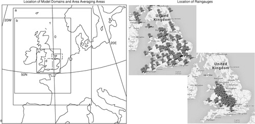
The western boundary of the nested 4 km run is shown to be very close to the boundary of the 12 km run; however, it meets the minimum suggested distance, eight gridlengths, for a nested model from the parent model's boundary Met Office (2008). No numerical errors or instabilities were observed due to the proximity of the two boundaries, as suggested may be present by other studies (e.g. Davies, 1983; Warner et al., 1997). Two separate 1.5 km runs were nested within the 4 km runs; one within the 4 km run which was nested within the 12 km run and the other within the 4 km run which was forced directly from the global model. A further 1.5 km run was also forced directly from the global model. The domain of the 1.5 km run was kept small to keep computational time manageable. As a result, the 1.5 km runs do not capture the whole of the extra-tropical cyclone, for either case study, but do capture the areas associated with the most extreme precipitation.

2.3. Observational data

To determine whether the downscaling method produces realistic intensities and distributions of the precipitation, the output from the LAM was compared to observational datasets. The observational data used in this study were raingauge data and radar data, with two separate raingauge datasets being available for the July event. A nationwide tipping bucket raingauge dataset was available via the UK Met Office Land Surface (MIDAS) dataset (UK Meteorological Office, 2012). This provides hourly accumulations for a few hundred raingauges throughout the UK from January 1915 to the present (Fig. 1, right, top). A further tipping bucket raingauge dataset was available for the July event from the UK Environment Agency (EA). This was only available on a per region basis for a specific (less than a month) time period but was at a higher spatial density than the MIDAS data (Environment Agency, 2011). As a result, the EA raingauges could only be obtained for a small area (Fig. 1, right, bottom). Both datasets, being tipping bucket data, record the time at which a bucket accumulates 0.2 mm of rain; these were then converted into hourly accumulations. For the intensities observed during these events, this equates to several tips an hour, representing a high temporal resolution, with a relatively small error.

The quality control flags from both the EA and MIDAS datasets were used to select only those raingauges that were not flagged as suspicious. The number of raingauges used in this study from each dataset is discussed in the next section. Neither of the raingauge datasets was available as a gridded dataset, which meant the comparison to the LAM output is made difficult. The option of creating a gridded dataset from either of the raingauge datasets, for example, via Kriging, was explored; however, the density of the MIDAS dataset was too low to produce a resolution useful for comparison to the LAM, and only two regions could be requested from the EA, again limiting the ability of creating a gridded dataset. The radar data used was the Met Office NIMROD data, a network of 15 C-band rainfall radars at a 2 km spatial resolution at a 5-minute temporal resolution. This was only used for the July event due to it being non-operational over the area for the June event.

2.4. Analysis methods

Due to neither of the raingauge datasets being gridded, none of the verification or skill scores methods, for example, Structure-Amplitude-Location (SAL, Wernli et al., 2008) or Fractional Skill Score (FSS, Roberts, 2008a), could be used to compare the LAM intensities to observations. The skill scores could not be used on the radar data either due to the radar data showing a very different distribution to the precipitation than seen in the model. The radar data had the precipitation organised in a line along the England–Wales border, whereas the models had the precipitation across southern England. The method chosen here was to take area averages within the LAM output and compare to the average raingauge intensity for all the raingauges and radar points that are located within this area. The size, and the location, of the averaging area was chosen to include the area in the model that showed the most intense precipitation, and designed to exclude areas with no precipitation, that is, including only the most intense precipitation seen in the LAM. For the July event this represented an area of around 40 000 km², and included 14 of the MIDAS raingauges and 29 of the EA raingauges. The June event was a much more localised event hence the averaging area was around 26000 km² and only including four of the MIDAS raingauges. The EA raingauges for this region were not able to be retrieved. These search areas are shown in Fig. 1 (left) as well as the location of the raingauges (right). The two raingauge datasets were kept separate for the July event due to the large differences in the density of the raingauges and the size of the areas covered by each dataset.

A further problem with comparing raingauge data to model data is that a raingauge is a point observation, whereas even a single grid box in the model will represent the average precipitation over an area determined by the resolution of the model. Areal Reduction Factors (ARFs), defined as ‘the ratio of rainfall depth over an area to the rainfall depth of the same duration and return period at a representative point in the area’ (Kjeldsen, 2007), have been used in the past to address this problem. The effect of ARF is essentially a bias correction to either the raingauge data or NWP data; however, Kjeldsen (2007) discuss that the ARF values expressed by Keers and Wescott (1977) have not been reviewed since 1977 and are expected to have changed in this time. Due to this reason, and it being unclear in Kjeldsen (2007) how ARF values should be applied to compare raingauge values to NWP data, ARF values are not used here.

In this study a cross-correlation method, which compares the location of maxima or minima between two data sets and determines whether the location of these are in the same place in each data set, is used. A cross-correlation was chosen over other methods as it was considered to provide the most useful information in regards to the difference in the location between areas of intense precipitation. The cross-correlation was used to compare the output between the lead times for all three resolution runs to determine whether the lead time resulted in the precipitation being in different locations. The cross-correlation is performed by initially aligning the two grids, normalising each data set, multiplying each grid point by the corresponding grid point in the other data set, and summing the results to gain a single value. The correlation, Corr(g, h), of two functions (data sets), g(x, y) and h(x, y) i s given by:1

where φ _x and φ _y are the offset in the x and y directions, respectively as the two grids are then staggered by repeatedly offsetting one grid relative to the other by one grid box, either in the x or y direction, and repeating this calculation. This value will be largest when the maxima (in the case of precipitation) are multiplied together in each grid. As the grids become more staggered, the rows and columns are wrapped so that the same number of grid points are taken each time, this wrapping has been masked in Fig. 6 to highlight the area of interest. The grids continue to be staggered until the two grids are completely offset, in both the x and y directions, creating a 2D image of values, with the x and y axes corresponding to the number of grid boxes the grids are offset by. If the two data sets have maxima in the same location, then the maximum value will appear at an offset of (0,0), indicating that no offset was required to align the areas of maximum precipitation. However, if the maximum value does not appear at (0,0), then it shows that the two data sets predict different locations for the maxima in the precipitation. The values have no units due to the normalisation of both fields prior to performing the cross-correlation. All of the cross-correlations were performed for the same area, 5.5° West to 0.5° East, 51° North to 54° North.

3. Event identification

During the Summer of 2007, England experienced extensive flooding due to precipitation associated with extra-tropical cyclones that passed over the UK on the 20th July and 25th June, resulting in widespread disruption affecting thousands of people (Pitt, 2008) in southern and north-east England, respectively. This section discusses the large-scale meteorological conditions that led to the intense precipitation events, the representation of the precipitation in the global model, and whether the large-scale meteorological conditions can be identified in the global model using a tracking algorithm. The July event is discussed first due to it being associated with more damage and disruption, and to a wider area, than the June event.

The precipitation experienced during the Summer of 2007 was unusual for summer events due to the persistent and widespread nature of the precipitation. Short lived, localised precipitation, associated with convective storms, is more typical during the summer months in the UK (Hand et al., 2004). The persistent and widespread nature suggests the presence of a larger-scale synoptic feature, however with convective cells embedded within the synoptic feature. This highlights the need to simulate such storms at resolutions more able to deal with convection, preferably at ‘storm resolving’ resolutions as discussed earlier.

The Hodges (1994, 1995) tracking algorithm (TRACK) was used to identify both events in the ECMWF Operational Analysis and to examine their lifecycles. This made use of 3 hourly data obtained by splicing 3 hourly forecasts between the 6 hourly analyses to provide higher frequency data. The results of the tracking can be seen in Fig. 2.

Fig. 2 The tracks of the July (left) and June (right) extra-tropical cyclone (blue) identified using the Hodges (1995) tracking method in the ECMWF Operational Analysis. For July, the green line shows a precursor storm that is considered to be associated with the main storm. The dates of the points indicated are at 0000.

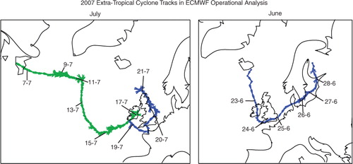
The track of the cyclone that caused the flooding during July (left, blue line) shows the cyclone originating over Ireland, curving south before moving north over the UK, along the east coast of England before disappearing off the north coast of Scotland. The green line represents another cyclone identified by TRACK, which shows a cyclone originating off the east coast of North America and travelling across the Atlantic. This track was included as it seemed to be associated with the July cyclone, and perhaps providing the precursor conditions for the July cyclone. The June event (right) is first identified off the coast of Iceland, from there it is tracked south crossing Ireland before turning east and moving along the south coast of England. It continued across Denmark and the south coast of Sweden and finally disappearing whilst over Finland. The most intense precipitation and the location of the flooding, for both events, occurred north of the storm centre due to the associated frontal system rotating north.

Using the ECMWF Operational Analysis, the lifecycles of the identified cyclones in terms of intensity measures of MSLP, 850 hPa vorticity and winds are examined and shown in Fig. 3. Also included is the total precipitation from the ECMWF Operational Forecast. To examine the full resolution properties of variables associated with the cyclones, their full resolution properties are added back onto the vorticity tracks using a search within a 5° spherical arc radius from the cyclones centre for each field. This was found to be sufficient to capture the extremes of the fields in the vicinity of the cyclone, as investigated for the wind field by Catto (2009) and for the precipitation (Champion et al., 2011). Precipitation is computed as the area average within this radius, the MSLP is calculated as the minimum within the 5° region, using a steepest descent minimisation. The 850 hPa maximum winds were obtained as a direct search for the maximum within the region as was the maximum vorticity at full resolution.

Fig. 3 Lifecycles of the July (top) and June (bottom) 2007 events, including the precursor event. The black line represents Mean Sea Level Pressure (MSLP, hPa), the blue line precipitation (precip, mm/hr), the red line winds (m/s) and the green line 850 hPa relative vorticity (vor, ×10⁻⁵/s), taken from the ECMWF Operational Analysis. The grey area is when the storm was over the UK.

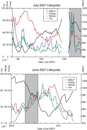
The July (Fig. 3, top) precursor event shows a strong cyclonic MSLP signal which weakens as it nears Ireland, with a strong wind signal although not a particularly strong precipitation signal; however, this is the average over a 5° area. This system may well have provided residual vorticity for the second storm to develop, as suggested by the 850 hPa relative vorticity field in the top plot of Fig. 3. As the second July event passes over England, shown as a grey shading, the pressure signal is not particularly strong, never dropping below 1000 hPa. The wind signal is also not very strong; however, a relatively high precipitation intensity is seen, with >0.7 mm/hr seen for a 5° area average, along with an increase in the relative vorticity. The precipitation intensity is an average over a 1×10⁶ km² radius and includes areas of no precipitation, hence a lower value; however, this is representative of intense precipitation.

The June (Fig. 3, bottom) event has a steadily deepening MSLP signal; however, whilst it is over the UK (grey shading) it is not a particularly deep signal although it is deeper than the July event. The winds, vorticity and precipitation signals intensify at the same time as the MSLP signal deepens, therefore the strongest signals are not seen whilst they are over the UK. Whilst over the UK, the winds associated with the June event are stronger than for the July event; however, the precipitation and vorticity signals are both weaker. As for the July event, the lifecycle of the June event suggests the presence of a large scale atmospheric feature; however, it is not a deep event in terms of MSLP.

The reason for the MSLP signal, for either event, not being very deep is as Blackburn et al. (2008) suggest, that the feature that caused the intense rainfall for both events were upper-level features, typically identified in the 200 hPa geopotential height field. These upper level features remained stationary over the UK due to an unusually persistent Rossby wave pattern on the mid-latitude jet stream, which was seen with the wave pattern being almost stationary around the entire Northern Hemisphere. The cyclones resulted in moist air being continually drawn from the Atlantic over land due to the cyclonic circulation resulting in a continual supply of water vapour which is important both for the development of the cyclones and for the production of precipitation. The role of the latent heat release caused by the precipitation has on the development of the cyclones is an interesting question which is not within the scope of this study. A closed, persistent, cyclonic circulation over the Atlantic, as is the case here, will result in a continual moisture supply moving from the Atlantic over the UK.

The presence of a large scale atmospheric feature, for example, an extra-tropical cyclone causing intense precipitation over a large area, is the focus of this study. To be able to predict where the precipitation will occur within a region such as the UK, and to determine which areas are likely to experience problems associated with the intense precipitation, high-resolution NWP models are required, even though the synoptic situation can be resolved quite well in a coarser resolution global circulation model. In the next section, the precipitation field from the LAM is analysed, to determine the optimal criteria for running the model and the impact of resolution on the precipitation intensity.

4. Results

The field of interest in this study is the precipitation field, a commonly investigated field in downscaling studies and also the principal, and sometimes the only, atmospheric variable used to drive hydrological models, therefore uncertainties associated in downscaled precipitation is likely to have a large impact on the output from the hydrological models. It is also the field with one of the smallest spatial scales, especially in the case of convective storms, and therefore the impact of an increase in resolution is likely to have a large effect on the results. The results are split up into the different areas of investigation in this study. First the way in which the LAM is configured is discussed, as it was found to have a big impact on the results. The results are then compared to observations to determine whether realistic precipitation intensities are obtained via this method. The July event was investigated first due to it being associated with more damage and disruption, and over a wider area, than the June event.

4.1. Choosing a re-initialisation frequency

Initially it was planned to run the LAM for an extended period, around 15 d, to capture the duration of the July storm and to try to capture both the rising limb and the falling limb of the precipitation, that is, the entire precipitation distribution associated with the storm. To run the model for such an extended period, the model was re-started (re-initialised) every 6 hours from the global model, the ECMWF Operational Forecast. However, this did not allow enough time for the precipitation to spin up from the initial state as the forecast model adjusts to the initial conditions, resulting in unrealistic precipitation intensities. The spin-up time was found to be between 6 and 12 hours, and therefore the model should not be initialised at a higher frequency than this. Boundary conditions were applied to the model every 6 hours to allow the global model to force the larger-scale pattern of the LAM.

Running the model using this method meant that the precipitation could spin-up, although the boundary conditions ensured that the global circulation continued to force the development of the larger-scale features within the LAM's domain. However, by removing the re-initialisation from the global model it was also found that the precipitation field became unrealistic 48 hours after the initialisation. For the purposes of this study, a 48 hour forecast was sufficient to capture the precipitation associated with the cyclones that caused the Summer 2007 flooding; the rising limb was captured in all the runs however the falling limb was not captured in the 48-hour lead time, although was captured in the other lead times. Therefore re-initialising the model every 48 hours to get the initially planned 15 d forecast was not explored. This does pose the question as to how frequently the LAM should be re-initialised for long timeseries runs of high-resolution, nested models; this is discussed in Section 5.

4.2. Temporal variation of the precipitation output

The uncertainty in the location of the precipitation over time was investigated by varying the lead time, the time between when the model was initialised, and the time the most intense precipitation is observed. If the location of the precipitation output from the different lead times is similar, then this suggests the uncertainty in the location of the precipitation is insensitive to lead time and therefore does not vary during the length of the forecast. In this study, the lead time is varied between 12 and 48 hours, in steps of 12 hours. By comparing the intensity, location and distribution of the precipitation field to observations, during the whole 48 hour forecast, will provide information as to whether the location of the precipitation remains constant between lead times, or varies during the 48 hour forecast.

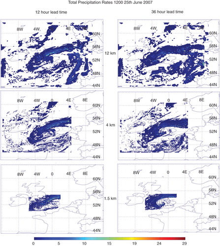
The precipitation field for the July event is shown in Fig. 4. This is the hourly accumulated precipitation field for 1200 on the 20th, when the peak in the precipitation was observed. Three resolutions are shown, the 12 km run (top), the nested 4 km run (middle) and the nested 1.5 km run (bottom), for forecasts started at two lead times, 12 hours (left) and 36 hours (right). Without using observations, this will show the effect of the lead time, and the resolution of the model, on the precipitation field.

Fig. 4 Total precipitation rates from the model at 1200 on the 20th July 2007 for the 12-hour lead time (left) and the 36-hour lead time (right), for the 12 km run (top), 4 km run (middle) and 1.5 km run (bottom). Units are mm/hr.

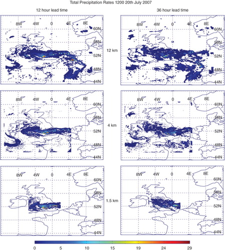
In the 12-hour lead time, a circulation of precipitation around the storm's centre, located between south Wales and Western England, is seen in all three runs, with the precipitation extending from Wales across England and down into France, although the domains of the 4 and 1.5 km runs do not extend into France. However, it is the distribution of the intense precipitation that changes between the runs, with the 12 km run predicting the intense precipitation to be further west and further north than in either of the other runs. The 4 km run and the 1.5 km show much greater agreement in the distribution of the precipitation to each other, although greater detail is seen in the 1.5 km run. Whether this greater detail is useful, or whether it is random noise, should be considered when using such high-resolution models for precipitation prediction; however, it is not explored here due to the use of area averages removing this detail.

The distribution of the precipitation is very different in the 36-hour lead time, for all three runs. The precipitation is not as intense, and the precipitation is shifted towards the east, most notably in the 1.5 km run where the area of most intense precipitation is over East Anglia. There is also a lot more variability between the runs in the 36-hour lead time. Whilst at this stage the field has not been compared to observations, see Section 4.5 where this analysis is undertaken, they cannot all have equal skill in predicting the location of the precipitation. This suggests that the uncertainties in the location of the precipitation field vary during the course of the forecast, due to the 12-hour lead time and 36-hour lead time runs showing different distributions. At the longer lead times the variation between the runs is also greater, compared to the variations between the runs at the shorter lead times. This would be expected as the runs are further away from the initial conditions; however, an important consideration when using downscaled precipitation is how the uncertainties associated with the precipitation will vary depending on how far through the forecast the precipitation occurs.

As already mentioned the forcing for the June event was much weaker, suggesting that the uncertainty in the location of the precipitation may be larger over time. The pattern of the precipitation is very different between the two lead times for the June event, Fig. 5. At a 36-hour lead time, there is more evidence of a cyclone centre being present over the UK, compared to a band of rain, more typical of a front, in the 12-hour lead time. The cause for the large difference in the structure of the rainfall is not clear. The effect of this is to change the location of the most intense precipitation, with the maximum intensity seen at a 36-hour lead time also being much lower than the maximum intensity seen at a 12-hour lead time. This large difference in the structure of the precipitation highlights that the uncertainty associated with the precipitation changes over time.

Fig. 5 Total precipitation rates from the model at 1200 on the 25th June 2007 for the 12-hour lead time (left) and the 36-hour lead time (right), for the 12 km run (top), 4 km run (middle) and 1.5 km run (bottom). Units are mm/hr.

4.3. Spatial variation in the precipitation output

The spatial variation in the precipitation output between the lead times was tested by performing a cross-correlation on the 12-hour lead time output to the 36-hour lead time output for an area covering most of England, shown in Fig. 6 for July (left) and June (right). This was not performed on the radar data due to the pattern being significantly different in the model compared to the radar, as discussed in Section 2.4. If the precipitation is in the same location for both lead times the maximum, shown in red, would be at (0,0). However, it can be seen that for all three resolutions the maximum in the cross-correlation occurs away from this centre point, indicating that the precipitation is in a different location in the two lead times.

Fig. 6 Cross-correlation between the precipitation fields from the 12-hour lead time and the 36-hour lead time for the 12 km (top), 4 km (middle) and 1.5 km (bottom) runs for July 2007 (left) and June 2007 (right). Red indicates a high correlation, blue shows a low correlation. The axes are the number of grid boxes shifted in each direction. The artificial periodicity is shown in the masked area.

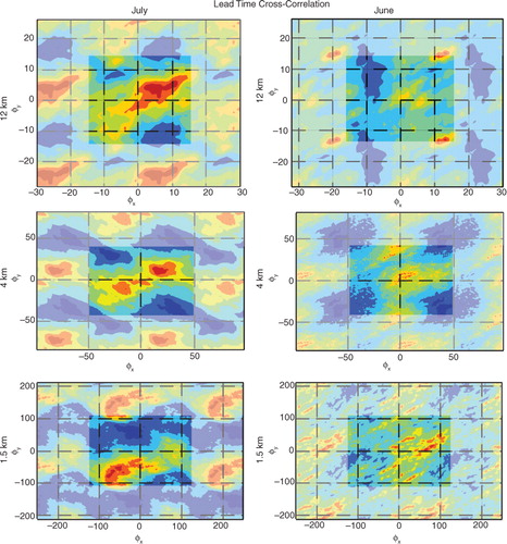
Figure 6 shows that there is a difference in the location of the most intense precipitation between the two lead times differing by 60 km for the 12 km run, 80 km for the 4 km run and 75 km for the 1.5 km run, either North-South or East-West. The July results (left) show larger areas of correlation, suggesting that the patterns of the precipitation are more similar between the lead times, compared to the June results (right). This will also be due to the extent of the precipitation which is much smaller for the June event. This uncertainty in the location of the intense precipitation at very high resolutions is to be expected and highlights the need to move towards a probabilistic approach to predicting the location of convective-scale events, rather than the deterministic approach used here (Roberts, 2008b). These results also highlight a significant problem for flood forecasting due to different catchments being affected dependent on the location of the precipitation.

4.4. Effect of downscaling on the precipitation field

If the uncertainties vary during the course of the forecast of the LAM, it could be argued that high-resolution global models, with no downscaling, may represent more useful precipitation information than downscaled precipitation, which is subject to various issues.

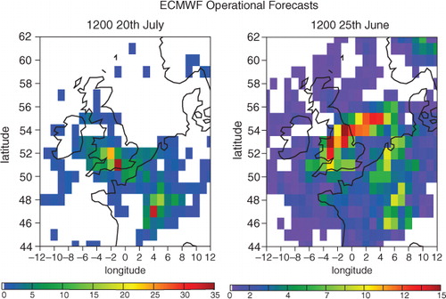
To compare the precipitation intensities from the global model to the LAM precipitation intensities, the precipitation field from the ECMWF forecast system is shown in Fig. 7 for July (left) and June (right). The forecast system is used, rather than the operational analysis data that is used to force the model, as precipitation is not an analysed quantity in the operational analysis system. To take into account the spin up, the 6-hourly accumulations for 1200 on the 20th July is calculated using the forecast started at 1200 on the 19th July, and subtracting the forecast for 1800 from the forecast for 0000 on the 20th July. The ECMWF Operational Forecast system in 2007 was at a 25 km resolution which is a coarser resolution than the LAM output. The accumulations predicted by the global forecast model are higher than those predicted by the LAMs, discussed in greater detail in the next section. The location of maximum precipitation is different in the global model compared to the LAMs. These results show that whilst the LAM is initialised by the global model, and is forced at the boundaries every 6 hours, it does produce different intensities and distributions to the precipitation in comparison to the global model. Whether these differences result in more accurate representations of the precipitation distribution and intensity is discussed in the next section. However, one benefit of downscaling, for hindcast events or from global models, is that the temporal resolution of the saved fields can be at a frequency more suitable for driving hydrological models without producing extremely large amounts of data.

Fig. 7 Six-hour precipitation accumulation for 1200 on the 20th July 2007 (left) and for 1200 on the 25th June 2007 (right) from the ECMWF Operational Forecast, the Operational Analysis was used to drive the LAM. Units are mm, the minimum accumulation shown is 0.5 mm.

This section has not compared the results to observations, however this section has explored the variation in the distributions and intensities of the precipitation field due to differences in the running method, that is, whether the run was nested within another high-resolution model or driven directly from the global data, and how far through the forecast the precipitation occurs, that is, the impact of lead time on the precipitation field. In the next section, the results are compared to rainguage data to determine which run and lead time produces distributions and intensities that most closely match observations.

4.5. Comparison with observations

It was shown in the previous section that the distribution, location and intensities of the downscaled precipitation are dependent on the lead time and downscaling method. In this section, the results are compared to observational data to provide information on whether a particular set up and lead time more closely matches observations than another. The datasets used are discussed in Section 2.3. As discussed in Section 2.4 ARFs, that have been used to compare point-source raingauge data to model data, are not applied here.

Figure 8 shows the area averaging comparison for July (top) and June (bottom) between the raingauges and the model for all three resolutions and two lead times. The first point to note is that the location of the averaging area is kept constant for each event, thus the fact that the lead times predict the precipitation to be in slightly different locations is not taken into account in this area averaging.

Fig. 8 Area averaged hourly precipitation rates for the model at a 12-hour lead time (black) and a 36-hour lead time (red) for resolutions at 12 km (solid), 4 km (dotted) and 1.5 km (dashed), and the average raingauge intensities (blue) for the MIDAS dataset (solid) and EA dataset (dashed, July only), for the July event (top) and the June event (bottom). The NIMROD data is shown as a dotted blue line (July only).

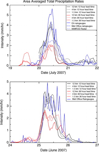
The July area averaged total precipitation for the 12-hour lead time runs (Fig. 8, black lines, top) have a similar time evolution for each of the model simulations compared to both raingauge datasets (blue lines), however there are differences in the intensities predicted. The timing of the peak in the precipitation differs between simulations and between datasets; the 12 km (solid line) and 1.5 km (dashed line) runs predict the peak in the precipitation to match the MIDAS raingauges whereas the 4 km (dotted line) run matches the EA raingauges (dashed line), an hour later. The radar data (blue dotted line) does not show such an obvious peak, however the maximum in the precipitation agrees with the EA data. There is a bigger disagreement between the model runs and raingauge observations in the falling limb of the precipitation, with both raingauge datasets showing a secondary peak a few hours after the main peak, however none of the model runs capture this secondary peak, nor is it captured in the radar data. This may have been a very localised convective system, too small to be identified in the model data and obscured in the radar data by other precipitation, however this was not investigated.

All of the July runs predict a steeper drop-off in the precipitation than the raingauge data. The cause for this is not known, it could be due to the raingauges recording random small-scale intense precipitation on a smaller scale than the model can resolve. For the peak precipitation, the 12 km run predicts the lowest area averaged intensity which is lower than the MIDAS data. The 4 and 1.5 km runs both predict intensities similar to the MIDAS data, all of which predict an area averaged intensity 1.5 mm/hr lower than the EA data for a period of several hours, therefore predicting a much lower cumulative precipitation total compared to the EA data.

The 36-hour lead time July runs (Fig. 8, red lines, top), at all three resolutions, have similar distributions around the time of peak precipitation, although noting that the 1.5 km run was only a 36 hour forecast due to computational limitations. The biggest variation is seen around midday on the 19th, that is, the day before the largest precipitation is observed. All three resolutions predict rainfall which isn't identified in either raingauge dataset. However, the 1.5 km run predicts more than double the amount of rainfall than either the 4 or 12 km runs. All three resolutions predict similar intensities for the peak in the precipitation on the 20th, although around 20% smaller than predicted by the MIDAS raingauge dataset, which observes a lower intensity than the EA raingauge dataset. The area average of the operational forecast (not shown) at the time of the peak precipitation is around 6.35 mm/hr, which is higher than the highest resolution runs. Compared with the current observations available this represents an over-estimation of the precipitation intensities. This suggests that the coarse resolution model can predict high intensities, as also seen in the LAM results, however they are not realistic when compared to observations. This is due to the forecast model predicting the intense precipitation to be over a much larger area than in the LAM due to the relatively coarse resolution of the forecast model.

It can be seen from Fig. 8 (July, top) that the two raingauge datasets used to compare to the July output predict different area average intensities. Whilst both datasets have a similar time evolution, it is apparent there is a large difference in the area average rate at the time of peak precipitation for the July event (1200 on 20th July), with the EA data showing an average around 5.5 mm/hr whereas the MIDAS data shows an average around 4 mm/hr. This is likely due to the number of raingauges included in the area averaging, due to differences in the spatial density of the two datasets. In the area averaging 14 MIDAS raingauges were included compared to the 29 EA raingauges that were within the averaging area. This increase in the number of gauges per given area increases the likelihood that small-scale precipitation, for example, convective cells, is captured.

The June area averaged total precipitation rates (Fig. 8, bottom) are noisier than the July event due to the smaller averaging area and more localised precipitation. The MIDAS observations (neither EA observations nor radar were available for the June event) are noisy due to only three raingauges being included in the averaging area, hence a clear peak in the precipitation cannot be seen. On average the 12 hour lead time runs (black lines) are closer to the observations (blue line) than the 36-hour lead time runs (red lines). The time evolution of the June rates is hidden by the noise although a similarly quick drop-off in the precipitation compared to the observations, as seen for July, can be observed. The June event highlights the issue of lead time but also shows all three resolutions predicting similar intensities and evolutions to the precipitation, highlighting the relative importance of the initial conditions. The area average of the operational forecast (not shown) at the time of peak precipitation shows significantly higher area average intensities, >11 mm/hr. This is again due to the forecast predicting the intense precipitation to be over a much greater area than the LAMs, although the extent of the intense precipitation predicted is much greater for the June event than the July event; however the LAMs predict an opposite pattern with the June event having a smaller extent than the July event. This highlights the need for an increased resolution of the model to improve the prediction of the small-scale features of such events.

5. Discussion and conclusions

This study has looked at the effect of the configuration when using a NWP LAM driven by data from a global model on the ability of the NWP model to produce realistic precipitation intensities and distributions for extreme precipitation associated with extra-tropical cyclones. This was done by looking at the precipitation field from the NWP model and comparing it to observational data. The study addressed the following questions:

What re-initialisation frequency can be used? In this study it was shown that it takes around 6 hours for the precipitation in the model to spin-up, meaning that a re-initialisation frequency of 6 hours or less would result in unrealistic intensities of precipitation. It was also found that after 48 hours the precipitation again became unrealistic, showing that boundary conditions do not provide enough constraint for the model to run for longer integrations. Therefore, for long downscaling integrations the model must be re-initialised at a minimum every 36 hours, and at a maximum every 12 hours. The precipitation data for the first 6 hours after re-initialisation would be unrealistic. This frequency may need to be reduced for events with weaker forcing; the cases here both have a strong large-scale feature associated with them for the entire period of the runs. The solution would be to have overlapping integrations, allowing the model to spin-up whilst the previous run is still producing realistic distributions, that is, re-initialising every 24 hours, running for 36 hours and not using the first 6 hours of data. Whether this dependence on the strength of the forcing is taken into account in timeseries downscaling is not clear, although it suggests that this will be a big factor on the uncertainties associated with the downscaled field.

How does the location uncertainty of the precipitation vary over time? By investigating the lead time, the time between initialising the model and the peak precipitation, it was shown that the uncertainties associated with the precipitation location increase during the 48 hour period, with the 12-hour lead time showing the best agreement to the low resolution raingauge data. This again shows the importance of the initial state. Roberts (2008b) noted that getting the location of storms correct is a big challenge, suggesting both resolution and the initial conditions have a large effect of the positions on storms. This result is of particular importance when using downscaled data as input to other models, for example, hydrological models that will need to take into account the changing uncertainty in the predictions.

What is the spatial variation in the precipitation output? The configuration of the downscaling was investigated by running the very high-resolution runs (4 km and 1.5 km) both by nesting them within a parent model and by running them directly from the global data, to determine whether the variation between the runs is more dependent on the driving data or the resolution of the run. The result of the nesting was for the location of the precipitation to be in similar locations for the different lead times, compared to when the runs were forced directly from the global data. This is likely due to stronger forcing from the nesting, compared to the boundary forcing from the global model. Roberts (2008b) suggest that the resolution of a model for such level of detail needs to be around 1–2 km where the convective parameterisations can also be switched off. The convective parameterisation was switched off for the 1.5 km run, where a lot more detail in the precipitation field is seen, and an increase in the area averaged precipitations intensities was seen. The accuracy of the extra detail produced by the 1.5 km run could not be assessed.

What is the effect of the density of the raingauge observations? Two raingauge products were used in the comparison for the July output and it was found that they differed in the observed intensities by up to 25%. This was attributed to the different sampling of the two products, with the EA data set having double the number of raingauges (29) than the MIDAS data set (14) for the July averaging area. The effect of a greater spatial density of the EA data is that the small-scale precipitation, for example, convective cells embedded within the larger scale precipitation, is captured in comparison to the coarser spatial density MIDAS data. However, only 29 EA raingauges were used for a 40000 km² area, which equates to less than one raingauge per 1000 km². This spatial scale is still larger than the scale of some convective cells, therefore it is possible that the EA data set does not capture all the convective cells and hence does not show the actual intensities experienced. The problems associated with using raingauge data as ‘truth’ are discussed by Thompson (2007). Neither data set was in a gridded format, and the option of gridding data was not within the scope of this study, which meant that to compare to the LAM output, an area within the LAM was averaged and compared to the average of all the raingauges that were in the same area.

What is the optimal set-up? The results suggest that a shorter lead time produces intensities which more closely match the lower resolution raingauge data set and highlights the importance of the initial conditions, although as discussed earlier, may also be due to the longer lead time predicting the precipitation to be in a different location. It appears that the optimal lead time from the start of the simulation to the peak intensity is roughly 12 hours to allow enough time for the precipitation to spin-up whilst ensuring there is still strong enough forcing from the initial conditions to constrain the model. Whilst the 36-hour lead time may simply be a spatial offset, greater variability between the runs was observed, and this still represents an error in the predicted precipitation and therefore a problem for catchment hydrology models.

The results also highlight the issue of resolution of the model. The small-scale nature of some of the precipitation during the storm means that a high resolution is required to capture the intense precipitation associated with such events. This was true for a large scale event, July 2007, as well as a more localised event, June 2007; however, both were caused by a large scale atmospheric feature. The results have shown that there is an optimal configuration for the model to predict precipitation intensities similar to the observations. This configuration is a short lead time, whilst allowing time for the precipitation to spin-up, with a series of nested resolutions to reduce the uncertainty in the precipitation over time.

The study has shown that realistic precipitation intensities can be obtained using a LAM driven from a coarse resolution global model, however with a specific configuration, and when compared to a relatively low resolution observational dataset. Whilst there is a need to test this configuration on a larger number of case studies, it would be possible to use this method to downscale information from a coarse resolution GCM to gain information at a more regional scale on the precipitation associated with extra-tropical cyclones in a warming climate. This is one of the aims of the NERC DEMON project and is similar to the approach taken by Mahoney et al. (2013) to investigate extreme precipitation events in a warmer climate in the Colorado Front Range. An extension to this work would be to investigate the dynamics of the extra-tropical cyclone at a high resolution during the entire lifetime of the cyclone. This could be achieved using a nested model whose domain moves with the centre of the cyclone, as used to investigate tropical cyclones (Tolman and Alves, 2005; Gopalakrishnan et al., 2012). Kühnlein et al. (2013) highlight the need to use an ensemble approach for convective-scale forecasts, where there is a weak large-scale forcing. The results from Kühnlein et al. (2013) show that after 6 hours it is the boundary conditions, and physics perturbations that dominate the uncertainty. If an ensemble approach was to be used here, it would extend the work on uncertainties presented in this study.

6. Acknowledgements

The authors acknowledge the help from Grenville Lister and Willie McGinty at NCAS Climate for help getting the limited area model running, and for the ECMWF for providing the global data. The raingauge data was provided by the UK Met Office (MIDAS) via the British Atmospheric Data Centre, and by the UK Environment Agency. The authors also thank the two reviewers for their comments on the paper.

References

- Bengtsson L. , Hodges K. , Keenlyside N . Will extratropical storms intensify in a warmer climate?. J. Clim. 2009; 22: 2276–2301.
- Blackburn M. , Methven J. , Roberts N . Large-scale context for the UK floods in summer 2007. Weather. 2008; 63: 280–288.
- Catto J . Extratropical Cyclones in HiGEM: Climatology, Structure and Future Predictions. 2009; Reading, UK: University of Reading. PhD Thesis.
- Champion A. , Hodges K. , Bengtsson L. , Keenlyside N. , Esch M . Impact of increasing resolution and a warmer climate on extreme weather from northern hemisphere extratropical cyclones. Tellus A. 2011; 63: 893–905.
- Chan S. , Kendon E. , Fowler H. , Blenkinsop S. , Ferro C. , co-authors . Does increasing the spatial resolution of a regional climate model improve the simulated daily precipitation?. Clim. Dyn. 2014; 41(5–6): 1475–1495.
- Cheng C. , Li G. , Li Q. , Auld H . A synoptic weather-typing approach to project future daily rainfall and extremes at local scale in Ontario, Canada. J. Clim. 2011; 24: 3667–3685.
- Davies H . Limitations of some common lateral boundary schemes used in regional NWP models. Mon. Weather Rev. 1983; 111: 1002–1012.
- Davies T. , Cullen M. , Malcolm A. , Mawson M. , Staniforth A. , co-authors . A new dynamical core for the Met Office's global and regional modelling of the atmosphere. Q. J. Roy. Meteorol. Soc. 2005; 131(608): 1759–1782.
- DEMON. 2012. Online at: http://www.bgs.ac.uk/stormrm/demon.html; http://www.bgs.ac.uk/stormrm/demon.html .
- ECMWF. IFS Documentation – Cy31r1 Part III: Dynamics and Numerical Procedures. 2007; Reading, UK: Technical Report. European Centre for Medium-Range Weather Forecasts.
- ECMWF. 2012. Online at: http://www.ecmwf.int/, URL http://www.ecmwf.int/ .
- Environment Agency. Hydrometry and Telemetry – How to Operate Rainfall and Climate Sites and Manage the Data. 2011; London, UK: Environment Agency. 1st ed. Operational instruction 622–11.
- Fowler H. , Blenkinsop S. , Tebaldi C . Linking climate change modelling to impacts studies: recent advances in downscaling techniques for hydrological modelling. Int. J. Climatol. 2007; 27: 1547–1578.
- Gopalakrishnan S. , Goldenberg S. , Quirino T. , Zhang X. , Marks F. , co-authors . Toward improving high-resolution numerical hurricane forecasting: influence of model horizontal grid resolution, initialization, and physics. Weather Forecast. 2012; 27(3): 647–666.
- Grahame N. , Davies P . Forecasting the exceptional rainfall events of summer 2007 and communication of key messages to Met Office customers. Weather. 2008; 63(9): 268–273.
- Gregory D. , Rowntree P . A mass flux convection scheme with representation of cloud ensemble characteristics and stability dependent closure. Mon. Weather Rev. 1990; 118: 1483–1506.
- Hand W. , Fox N. , Collier C . A study of the twentieth-century extreme rainfall events in the United Kingdom with implications for forecasting. Meteorol. Appl. 2004; 11: 15–31.
- Hodges K. I . A general method for tracking analysis and its application to meteorological data. Mon. Weather Rev. 1994; 122: 2573–2586.
- Hodges K. I . Feature tracking on the unit sphere. Mon. Weather Rev. 1995; 123: 3458–3465.
- Keers J. , Wescott P . A Computer-Based Model for Design Rainfall in the United Kingdom. 1977; Exeter, UK: Met Office, Met Office Scientific Paper No. 36.
- Kendon, E., Roberts, N., Senior, C. and Roberts, M. 2012. Realism of rainfall in a very high-resolution regional climate model. J. Clim. 25, 5791–5806. DOI: 10.1175/JCLI-D-11-00562.1.
- Kjeldsen T . Flood Estimation Handbook Supplementary Report No. 1: The Revitalised FSR/FEH Rainfall-Runoff Method. 2007; Wallingford, UK: Centre for Ecology and Hydrology, Supplementary Report No. 1.
- Kühnlein C. , Keil C. , Craig G. , Gebhardt C . The impact of downscaled initial condition perturbations on convective-scale ensemble forecasts of precipitation. Q. J. Roy. Meteorol. Soc. 2013
- Lean H. , Clark P. , Dixon M. , Robers N. , Fitch A. , co-authors . Characteristics of high-resolution versions of the met office unified model for forecasting convection over the united kingdom. Mon. Weather Rev. 2008; 136: 3408–3424.
- Lo J. C.-F. , Yang Z.-L. , Pielke R . Assessment of three dynamical climate downscaling methods using the Weather Research and Forecasting (WRF) model. J. Geophys. Res. 2008; 113: D09112.
- Mahoney K. , Alexander M. , Scott J. D. , Barsugli J . High-resolution downscaled simulations of warm-season extreme precipitation events in the Colorado front range under past and future climates. J. Clim. 2013; 26: 8671–8689.
- Met Office. Unified Model User Guide. 2008; Exeter, UK: Met Office. 4th ed.
- Orskaug E. , Scheel I. , Frigessi A. , Guttorp P. , Haugen J. , co-authors . Evaluation of a dynamic downscaling of precipitation over the Norwegian mainland. Tellus. 2011; 63(4): 746–756.
- Osborn T. , Hulme M. , Jones P. , Basnett A . Observed trends in the daily intensity of united kingdom precipitation. Int. J. Climatol. 2000; 20: 347–364.
- Pinto J. , Ulbrich U. , Leckebusch G. , Spangehl T. , Reyers M. , co-authors . Changes in storm track and cyclone activity in three SRES ensemble experiments with the ECHAM5/MPI-OM1 GCM. Clim. Dyn. 2007; 29: 195–210.
- Pitt M . The Pitt Review: Learning Lessons From the 2007 Floods. 2008; London, UK: Technical Report. Cabinet Office.
- Roberts N . Assessing the spatial and temporal variation in the skill of precipitation forecasts from an NWP model. Meteorol. Appl. 2008a; 15: 163–169.
- Roberts N . Modelling Extreme Rainfall Events. 2008b; London, UK: Department for Environment and Rural Affairs. Technical Report.
- Thompson R . Rainfall Estimation Using Polarimetric Weather Radar. 2007; Reading, UK: University of Reading. PhD Thesis.
- Tolman H. L. , Alves J.-H. G. M . Numerical modeling of wind waves generated by tropical cyclones using moving grids. Ocean Model. 2005; 9: 305–323.
- Trémolet Y . Incremental 4D-Var Convergence Study. 2005; Reading, UK: ECMWF. Technical Report 469.
- Tryhorn L. , DeGaetano A . A comparison of techniques for downscaling extreme precipitation over the Northeastern United States. Int. J. Climatol. 2011; 31: 1975–1989.
- UK Meteorological Office. Met office integrated data archive system (Midas) land and marine surface stations data (1853-current). 2012. Online at: http://badc.nerc.ac.uk/view/badc.nerc.ac.uk__ATOM__dataent_ukmo-midas; http://badc.nerc.ac.uk/view/badc.nerc.ac.uk__ATOM__dataent_ukmo-midas .
- Warner T. , Peterson R. , Treadon R . A tutorial on lateral boundary conditions as a basic and potentially serious limitation to regional numerical weather prediction. Bull. Am. Meteorol. Soc. 1997; 78(11): 2599–2617.
- Wernli H. , Paulat M. , Hagen M. , Frei C . SAL – a novel quality measure for the verification of quantitative precipitation forecasts. Mon. Weather Rev. 2008; 136: 4470–4487.
- Wilson D. , Ballard S . A microphysically based precipitation scheme for the UK Meteorological Office unified model. Q. J. Roy. Meteorol. Soc. 1999; 125: 1607–1636.