Prior history of Mistral and Tramontane winds modulates heavy precipitation events in southern France

Abstract

Heavy precipitation events (HPEs) are frequent in southern France in autumn. An HPE results from landward transport of low-level moisture from the Western Mediterranean: large potential instability is then released by local convergence and/or orography. In the upstream zone, the sea surface temperature (SST) undergoes significant variations at the submonthly time scale primarily driven by episodic highly energetic events of relatively cold outflows from the neighbouring mountain ranges (the Mistral and Tramontane winds). Here, we study the HPE of 22–23 September 1994 which is preceded by a strong SST cooling due to the Mistral and Tramontane winds. This case confirms that the location of the precipitation is modulated by the SST in the upstream zone. In fact, changes in latent and sensible heat fluxes due to SST changes induce pressure and stratification changes which affect the low-level dynamics. Using three companion regional climate simulations running from 1989 to 2009, this article statistically shows that anomalies in the HPEs significantly correlate with the SST anomalies in the Western Mediterranean, and hence with the prior history of Mistral and Tramontane winds. In such cases, the role of the ocean as an integrator of the effect of past wind events over one or several weeks does indeed have an impact on HPEs in southern France.

• heavy precipitation events
• Mediterranean
• Mistral
• air–sea interactions
• CORDEX
• atmosphere–ocean coupling

To access the supplementary material to this article, please see Supplementary files under Article Tools online.

1. Introduction

In autumn, the Mediterranean coasts are often prone to heavy precipitation events (HPEs) (typically more than 100 mm in 24 h) that can lead to flash floods. These situations are generally linked to the presence of cold air in altitude blocked over the Iberic Peninsula that induces a rapid diffluent southerly flow in the upper layer over Western Europe. HPEs frequently occur in southern France when low-level southerly winds advect warm and moist air towards hilly topography such as the Cévennes (the southern part of the Massif Central, Fig. 1). The convective available potential energy is then at a maximum. Mountains or wind convergence on the sea allow the triggering and enhancement of convection. When local feedbacks are at play and/or when synoptic conditions evolve slowly, convective systems can become stationary and can lead to severe flash floods (Ducrocq et al., 2008; Nuissier et al., 2008).

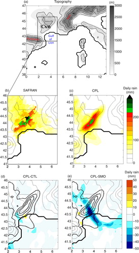
Fig. 1 Topography and rivers of the region including the western Mediterranean with geographical indications and definition of boxes used to calculate averaged SST differences in the IPSS calculation (see Section 4): GoL includes the plateau of the Gulf of Lion, Py the area offshore of the Pyrenees, Ba the area between the Balearic Islands and the Spanish coast, Li the Ligurian Sea extended down to the north of Sardinia, South Med the area between the Balearic Island and Sardinia and Ty the Tyrrhenian sea.

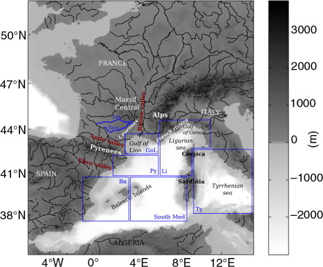
The Cévennes are separated from the Alps to the east by the Rhône valley and from the Pyrenees to the west by the Aude valley (Fig. 1). This layout is such that the region is also subject to strong winds when westerly to northerly winds blow across France. In fact, the flow is then channelled by the valleys in southern France and accelerates: the Mistral (Drobinski et al., 2005; Guénard et al., 2005, 2006) and the Tramontane (Drobinski et al., 2001) blow respectively from the Rhône and the Aude valleys. These winds are particularly cold and dry, inducing strong evaporation over sea and the whole north-western Mediterranean can cool by a few degrees when they blow for several days in autumn. The Gulf of Lions is located just south of the Cévennes, where strong northerly wind and intense air–sea flux enhance the oceanic cyclonic circulation (Madec et al., 1996) with mixing and entrainment in addition to cooling of the sea surface (Lebeaupin Brossier and Drobinski, 2009). The deepening of the oceanic mixed layer in autumn is a pre-conditioning of strong deep convection around 42°N–5°E that can occur in winter (Marshall and Schott, 1999; Béranger et al., 2010). The sea surface temperature (SST) in the Gulf of Lions can thus change from 20°C in summer to 13°C in winter (Fusco et al., 2003).

If such strong air–sea interaction events occur before a precipitation event, the cooling of the sea can be such that it induces changes in the thermodynamic properties of the atmosphere when southerly winds blow over it towards the Cévennes. In fact, the Mediterranean Sea can directly contribute to the heat and moisture feeding of the systems (Millán et al., 1995; Duffourg and Ducrocq, 2011) and changes in the SST can change the precipitation amounts of HPE (Pastor et al., 2001; Homar et al., 2002; Lebeaupin et al., 2006; Lebeaupin Brossier et al., 2013; Berthou et al., 2014).

Regional climate modelling allows multi-decadal timescale simulations at higher resolution compared to global climate modelling. These systems now reach spatial resolution (10–25 km) that allow the simulation of strong precipitation events (Colin, 2012; Rajczak et al., 2013). However, local processes and feedbacks involved in the dynamics of mesoscale convective systems cannot be fully represented in regional climate models (RCMS), because of the convection parameterisation and the insufficient resolution of complex terrain. Nevertheless, HPEs mainly driven by synoptic conditions are well reproduced. RCMs can thus be used to study the evolution of extreme events with climate change in regions of relative fine scale topography and land–sea contrast (Giorgi et al., 2009). Finally, RCMs tend to be multi-compartment systems, which integrate coupling with the ocean and land-surface for example. In this study, we use an Atmosphere–Ocean Regional Climate Model (AORCM). It allows the study of air–sea interactions and coupled processes, which are especially strong in the north-western Mediterranean.

Lebeaupin Brossier et al. (2013) compared a simulation of an RCM forced by ERA-interim SST with an AORCM on an intense precipitation event in the Aude valley on 12–13 November 1999. Seven days before precipitation occurred, a strong Mistral event started and lasted 5 d. The event decreased the SST by 1°C on average over the Gulf of Lions (and locally by 2°C) while only a mean decrease was present in the ERA-interim SST field of the RCM simulation. This difference led to an eastward shift in precipitation in this AORCM compared to the RCM. However, through the direct comparison of an RCM with an AORCM, two effects could not be separated: the proper coupling effect at submonthly scales and the effect of long-term biases in the SST. Then, Berthou et al. (2014) used a third simulation: an RCM forced by the SST coming from the AORCM which had been smoothed over a month to remove the effect of the SST biases and keep only the submonthly air–sea coupling effects. The study focused on the HPE of 19 September 1996 that showed major changes in the precipitation distribution due to large long-term biases between the RCM and the AORCM in the Gulf of Lions. Only a minor part of the difference was due to proper air–sea coupling since no major Mistral event occurred before the precipitation event. The difference in precipitation mainly originated from differences in the wind field and not in the water vapour or Convective Available Potential Energy fields. Small et al. (2008) indicate in fact that in the mid-latitudes, mesoscale eddies and SST fronts can have an influence on dynamic fields through modifications of the pressure field, atmosphere stability and surface friction.

The aim of this paper is to study the submonthly air–sea coupling impact on a HPE. Thus, we first tackle another HPE, 22–23 September 1994 where the precipitation differences mainly come from submonthly coupled effects, to understand what mechanisms are at play in the precipitation change. In light of this case study and of Berthou et al. (2014), an index is proposed to quantify when HPEs are most sensitive to submonthly air–sea coupling and to biases in SST.

Section 2 introduces the models and simulations that are used. In Section 3, the HPE is described as well as the pre-conditioning of the SST. A comparison of the different simulations is performed and an explanation of the precipitation differences is given. Section 4 explains the construction of an index relating precipitation differences to SST differences and tests this index on the two most extreme precipitation events simulated by the RCM in the 1989–2009 period. The last section summarises the advances made possible by the study and discusses possible follow-ups.

2. Materials and methods

The model set-up is the same as in Lebeaupin Brossier et al. (2013) and the simulations are also used in Berthou et al. (2014), so the description can also be found in these articles.

2.1. Experimental design

The MORCE (Model of the Regional Coupled Earth system) platform is the framework in which the regional two-way air–sea coupled system (the AORCM) used in this study was developed (Drobinski et al., 2012). It is a tool to better understand the role of coupled processes on the regional climate of particularly vulnerable areas. The MORCE system is used in the Hydrological Cycle in the Mediterranean Experiment (HyMex) (Drobinski et al., 2014) and the Coordinated Downscaling Experiment (CORDEX) of the World Climate Research Program (WCRP) (Giorgi et al., 2009).

2.1.1. The atmospheric model.

The atmospheric model within the MORCE system is the Weather Research and Forecasting (WRF) model of the National Center for Atmospheric Research (NCAR) (Skamarock et al., 2008). The domain covers the Mediterranean basin with a horizontal resolution of 20 km. It has 28 vertical levels using sigma coordinates. The first 1000 m are resolved on eight levels. Initial and lateral conditions are taken from the European Centre for Medium-Range Weather Forecasts (ECMWF) ERA-interim reanalysis (Simmons et al., 2007) provided every 6 h with a 0.75° resolution. Moreover, indiscriminate nudging is used to constrain the fields above the planetary boundary layer with a coefficient of 5.10⁻⁵s⁻¹ for temperature, humidity and velocity components. This reduces chaos between different simulations and allows us to consider that the differences come mostly from the surface differences (Stauffer and Seaman, 1990; Salameh et al., 2010; Omrani et al., 2013). The nudging is a Newtonian-type nudging with relaxation towards ERA-interim reanalysis. The nudging coefficient was chosen following Omrani et al. (2013) so that the relaxation time is large enough to constrain the large scale more than the small scale since the large-scale evolution is slower. The boundary layer parametrisation is a K-profile scheme improved by Noh et al. (2003) (YSU). The surface-layer is the Monin-Obukov scheme (Stull, 1994).

The cumulus convection scheme is the Kain-Fritsch scheme (Kain, 2004). Convection is triggered when the temperature of a 60 hPa layer is higher than the environment temperature at its condensation level. A temperature deviation is added to the parcel depending on the larger scale vertical velocity in order to trigger convection in a converging environment. The updraft initial velocity depends on the buoyancy difference with the environment at the lifting condensation level. The updraft velocity is then influenced by entrainment, detrainment and water loading. If the updraft reaches a minimum cloud depth, which depends on the base cloud temperature, deep convection is triggered. Otherwise, the algorithm proceeds to the same test with the 60 hPa layer one level above the former one and the algorithm goes on. Convective updrafts are represented using a steady-state entraining/detraining plume model where entrainment and detrainment rates are inversely proportional. Downdraft mass flux is estimated as a function of the relative humidity and stability just above cloud base. Downdraft stops when it reaches the surface or when it becomes warmer than the environment. It is then forced to detrain into the environment within and immediately above the termination level. The convection stops when the CAPE calculated for a parcel with entrainment is consumed.

The complete set of physics parametrisations can be found in Lebeaupin Brossier et al. (2013).

2.1.2. The ocean model.

The ocean model of MORCE is Nucleus for European Modelling of the Ocean (NEMO) (Madec and the NEMO Team, 2008). It is used in a regional eddy-resolving Mediterranean configuration MED12 (Lebeaupin Brossier et al., 2011; Beuvier et al., 2012) with a 1/12° horizontal resolution, which represents about 6.5–7 km in the Gulf of Lions. In the vertical, MED12 has 50 stretched z-levels with finer resolution near the surface. The initial conditions for 3D potential temperature and salinity fields are provided by the MODB4 climatology (Brankart and Brasseur, 1998) except in the Atlantic zone between 11°W and 5.5°W, where the Levitus et al. (2005) climatology is applied. In this area, a 3D relaxation to this monthly climatology is used. River runoff and the Black Sea water input come from a climatology and their freshwater flux is set at the mouths of the 33 main rivers and at the Dardanelles Strait respectively. Smaller river runoffs are summed and set as a homogeneous coastal runoff around the Mediterranean Sea as in Beuvier et al. (2010). Further details on the ocean model parametrisation can be found in Lebeaupin Brossier et al. (2013) and Beuvier et al. (2012).

2.1.3. Numerical experiments.

The control simulation (CTL) is the downscaling of the ERA-interim reanalyses obtained with WRF alone. For this RCM simulation, the SST is thus prescribed from ERA-interim and is updated daily.

The coupled simulation (CPL) runs with two-way interactive exchanges between the two compartment-models managed by the OASIS coupler version 3 (Valcke, 2006). For this AORCM simulation, the exchanged variables are the SST and the heat, water and momentum fluxes. The coupling frequency is 3 h. The coupler uses a bilinear method to interpolate the ocean grid towards the atmospheric grid and vice versa.

The smoothed simulation (SMO) is an atmosphere-only simulation with the same characteristics as the CTL simulation, except that instead of the ERA-interim SST, a new SST field has been used for the forcing of the atmospheric model. This forcing has been designed in order to retain the same climatology and diurnal cycle as the CPL SST, but without the submonthly SST variations. For that purpose, the SST value used to force the RCM at each target time step was calculated by performing a central moving average with a 31-d window, retaining only the 31 time steps in the time window that correspond to the same GMT time as the target time step. This way, the diurnal cycle (as well as its seasonal variations) is preserved, as are all the persistent spatial structures that exist in CPL. The high-frequency air–sea coupling effects (submonthly variations), however, are not present in SMO.

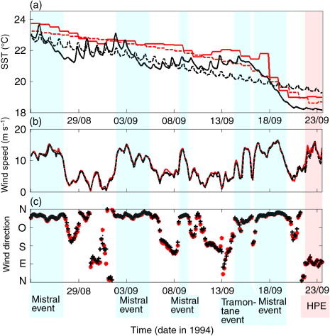
The three simulations run from January 1989 to December 2008. CPL starts with an ocean at rest. In this study, we only focus on the north-western Mediterranean area in September 1994. Figure 2 illustrates the differences in SST between the three simulations during the month preceding the precipitation event of 23 September 1994 averaged on the Gulf of Lions (Fig. 1). CPL SST shows a daily cycle and sudden decreases of SST on several days. The SST of SMO simulation shows a smoothed evolution over the month. The CTL SST lacks a daily cycle since it is updated daily. It also shows a smooth evolution but the large cooling of 14–19 September is represented.

Fig. 2 (a) Time evolution of the SST (°C) averaged over the box GoL defined in Fig. 1. GOS-SST (red line), CTL: ERA-interim at 0.75° (red dashed line), CPL: from NEMO (black line), SMO (black dashed line); (b) wind intensity and (c) wind direction for CPL (black line) and CTL (red line) at (42.4°N–5°E).

3. Chronology of the Mistral event and representation of the HPE

3.1. Pre-conditioning of the SST: Mistral/Tramontane events

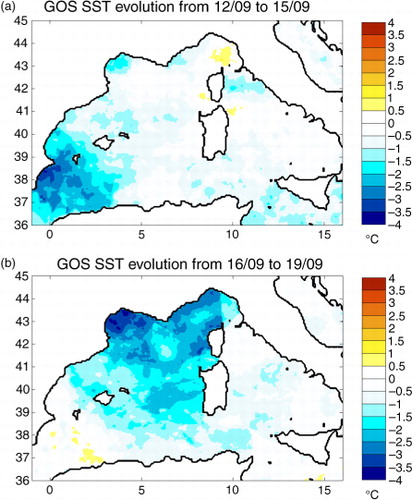
Over the month preceding the precipitation event, the GOS-SST, which is an optimally interpolated SST with a resolution of 1/16°obtained from the night-time satellite data of the Advanced Very High Resolution Radiometer (Marullo et al., 2007), shows four periods of strong cooling (Fig. 2a). For each period, the CPL simulation also represents a cooling that is associated with northwesterly to northerly winds at (42.4°N, 5°E) with an intensity greater than 10 ms⁻¹, respectively, the Tramontane and the Mistral (Fig. 2b and c). Thus, the CPL simulation is able to reproduce those strong air–sea coupling events. The last and strongest Tramontane and Mistral event started on 14th of September. Strong westerly winds lasted 2 d and reached the Gulf of Genoa: the Tramontane blew from the Aude valley and the Cierzo from the Ebro valley. It cooled the SST in the Gulf of Lions and offshore the French Riviera by 1.4°C and 0.6°C, respectively (Fig. 3a). On 16th, the Tramontane ended and a short transition took place with weaker winds before the Mistral started at the end of the day. Northerly winds of up to 20 ms⁻¹ in the model blew for 3 d until 19th (Fig. 2b and c). The GOS-SST cooled down by 3°C on average in the Gulf of Lions (Fig. 2a) and by 2.5°C in the French Riviera (Fig. 3b). Moreover, the Mistral affected the whole western Mediterranean basin since the SST cooled down by about 0.5°C near the Algerian coast (Fig. 3b). From 20^th to 23^rd, the SST did not show much evolution (Fig. 2a).

Fig. 3 Effect of the successive Tramontane and Mistral events in high-resolution reanalyses GOS-SST: (a) SST difference between 15 and 12 September 1994 during the Tramontane event (°C); (b) SST difference between the 19 and 16 September 1994 (°C) during the Mistral event.

The CPL simulation reproduces the intensity of the cooling in the Gulf of Lions with an overestimation of 0.5°C compared to GOS-SST. The coupling of an atmospheric regional model with 20 km resolution with an ocean model of the Mediterranean Sea with 6–7 km resolution is thus successful in representing the air-sea coupling under such a strong and long-lasting wind event. Locally, it shows too strong a cooling in the Gulf of Genoa compared to GOS-SST (Fig. 4a and b). The SST of ERA-interim that was used in CTL simulation also shows good representation of the cooling in average in the Gulf of Lions (Fig. 2a). However, the preceding smaller air–sea coupling events are not represented by ERA-interim SST, as it was also noticed in Berthou et al. (2014) on the case of 16 September 1996. The CPL simulation also shows differences with the CTL simulation of about 1°C north of Corsica and −2.5°C south of the Pyrenees (Fig. 4c).

Fig. 4 Sea surface temperature on 23 September 1994 (°C): (a) SST from NEMO-MED12 in CPL simulation (daily mean); (b) SST in GOS fine scale reanalyses; (c) difference between CPL and CTL simulations (daily mean); (d) difference between CPL and SMO simulations (daily mean).

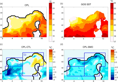
The SMO simulation shows a smoothed cooling that represents the trend of September (Fig. 2a). Thus, it does not show the air–sea coupling effects that are responsible for the SST cooling from 14th to 19th shown by CPL and CTL. Therefore, the difference between CPL and SMO shows the effect of submonthly air–sea coupling. On 23rd, Fig. 4d shows that CPL is colder than SMO on the whole north-western Mediterranean by 0.6°C with a maximum cooling along the French Riviera that reaches −2°C. This is due to the strong Mistral/Tramontane event that SMO simulation does not take into account.

To sum up the differences between the three simulations, the CPL simulation shows an SST response to this Tramontane and Mistral event that SMO does not have because of its construction. CTL also reproduces the effect of the last Mistral event on the SST but shows in addition to it a long-term SST difference with CPL. When the winds change direction and blow towards the Cévennes, the SST is thus different in the three simulations and can induce differences in the atmospheric fields.

3.2. The HPE of 22–23 September 1994

On 22 and 23 September 1994, a cut-off low indicated by the 500 hPa geopotential height stays during the 2 d over Spain (not shown). A surface depression is located over Spain and evolves slowly towards the northeast. Consequently, southeasterly winds blow over the Mediterranean, bringing warm, moist and unstable air towards southern France. Thunderstorms develop in the Gulf of Lions and heavy precipitation occurs on the Cévennes in the morning of 22nd (also shown by the model in Fig. 5). On 23rd, moderate rain starts in the morning and turns into heavy rain on the Gulf of Lions and the Cévennes. Cumulated rain over the 2 d led to major floods of the rivers Lot and Rance (tributary of the river Tarn, Fig. 1) with damage reported on buildings (RIC, 2012).

Fig. 5 Precipitation cumulated every 3 h (RR3) averaged over the Cvn box shown in Fig. 6a. Cv=convective rain (resulting from the parametrisation scheme), non Cv=rain resulting from resolved processes in CTL, CPL and SMO simulations; no graupel was recorded.

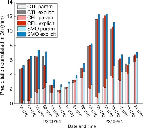
Figure 6b shows the accumulated rainfall over the 2 d (22 and 23 September 1994) in the SAFRAN analysis which provides 8 km gridded rain at the hourly time step using ground data observations (raingauges) (Quintana-Seguí et al., 2008). The cumulated rainfall extends along the Cévennes and presents two local maxima: to the east (44.36°N,3.75°E), raingauges report 323 mm in Le Pont-de-Montvert and to the west (43.9°N, 3.1°E), raingauges report up to 251 mm in Fondamente. In comparison to SAFRAN, the spatial extent of the rain in the CPL simulation is well reproduced on the slopes of the Cévennes along the 500 m terrain-height: two local maxima are represented with 220 mm of rain just south of the two SAFRAN maxima (Fig. 6c). However, it lacks accuracy away from the slopes. The SMO simulation produced 40 mm more rain than the CPL simulation between the two CPL maxima. Thus, SMO shows only one maximum of 284 mm at (44°N, 3.5°E) and overestimates precipitation in the zone between the two SAFRAN maxima by more than 100 mm. Figure 5 shows that this increase occurs throughout the 2 d and is mainly an increase in rain resulting from the cumulus convection scheme. The CTL simulation (Fig. 6d) shows little difference with the CPL simulation (−10 mm in 2 d).

Fig. 6 (a) The north-western Mediterranean region as represented by WRF model at 20 km resolution (topography with contours every 500 m); (b,c) accumulated precipitation over the 22 and 23 September 1994 (mm). (b) In SAFRAN/F analysis at 8 km resolution using ground data observations. (c) In CPL; (d,e) CPL 2 d-accumulated precipitation (contour every 50 mm), colours: Rain difference cumulated over the 2 d between. (d) CPL and CTL simulations and (e) CPL and SMO simulations.

Thus, CPL shows some improvement in the rain location compared to SMO owing to submonthly coupling of the atmospheric model to an oceanic model in CPL. The CTL simulation performs similarly to CPL. The fact that there are more differences in the rain field between CPL and SMO than between CPL and CTL while there are large SST differences in both cases will be discussed later in Section 4. Focus is now on the explanation of CPL-SMO precipitation difference.

3.3. Rain differences induced by the submonthly coupled effects on 22–23 September 1994

CPL simulation shows 40 mm less precipitation in the middle of the Cévennes than SMO simulation and 30 mm less in the Gulf of Lions (Fig. 6e). This rain difference occurs mainly during the two convergence episodes that occurred on the morning of 22nd and of 23rd. Both situations are illustrated in Figs. 7a, c and 8a, c. Figure 7c shows a decrease in precipitation on 22 September at 03 UTC by 8 mm east of the precipitation maximum (30 mm) and an increase by 2 mm west of it. This is a similar situation to 19 September 1996 shown in Berthou et al. (2014) where a shift of the peak of precipitation was observed between CPL and CTL simulations. It corresponds to wind changes in the convergence zone, as shown in Fig. 7a and b. Figure 7d shows a pressure anomaly higher than 0.5 hPa located at (43.5°N, 4.1°E) in a convergence zone between strong southeasterly winds blocked by the Alps (Fig. 7a) and northeasterly winds coming from the Rhône valley. The pressure anomaly is hydrostatic: temperature anomalies due to SST anomalies on the wind path (Fig. 4d) accumulate vertically in the convergence zone, leading to this enhanced pressure anomaly. The same phenomenon can be observed at (42.4°N, 6°E) with a smaller pressure anomaly. The first pressure anomaly may be linked to the anticyclonic shift of the wind seen from (42.75°N, 4°E) to (43.3°N, 3.5°E) (Fig. 7b). The wind on the eastern side of the convergence zone gets a stronger southeast component which leads to a westward shift of the convergence maximum, reducing the rain on the eastern side of the convergence zone and enhancing it on the western side.

Fig. 7 Situation on 22 September 1994 at 03 UTC on the Gulf of Lions (a) wind at first level (shading: CPL intensity, black arrow: SMO wind vector, red arrow: CPL wind vector); (b) difference in first level wind between CPL and SMO (shading: wind intensity, black arrow: wind direction); (c) colour: Rain difference between CPL and SMO cumulated from 00 to 03 UTC (mm), contour: CPL rain (every 10 mm/3 h); (d) colours: difference in first level pressure between CPL and SMO (hPa), dashed-line: wind divergence lower than zero (every 2.5.10⁻⁵s⁻¹); (e) Moist Brunt-Väisälä frequency averaged on the first five levels of atmosphere for CPL (10⁻³s⁻¹), (f) Difference in moist Brunt-Väisälä frequency averaged on the first five levels of atmosphere between CPL and SMO (10⁻³s⁻¹).

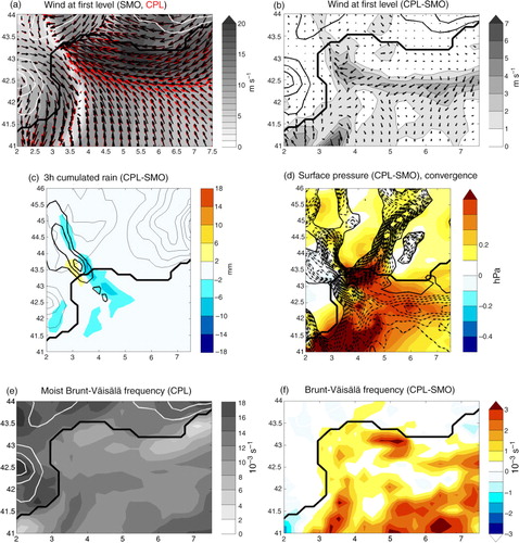
The weaker convergence zone with a west–east orientation axis at 42.4°N is also affected by a wind change (Fig. 7a and b): the south to south-southeasterly wind is more deviated to the west when it encounters this convergence zone in CPL than in SMO. This zone of convergence is the limit of the area where the winds are blocked by the Alps and deviated to the west in a strong easterly low-level jet. Thus, the blocking of the Alps is more efficient in CPL than in SMO. This can be linked to an increase in the temperature stratification in the area south of the blocking zone owing to cooler SST. In the zone around (41.5°N, 6°E), the moist Brunt-Väissälä frequency is 10×10⁻³s⁻¹ in CPL (Fig. 7e), this is 2×10⁻³s⁻¹ larger than in SMO (Fig. 7f). In fact, this leads to an increased Froude number from 2.1 to 2.5 [Fr=Nh _m /U where N is the moist Brunt-Väisälä frequency, h _m the mountain height (2500 m) and U the upstream wind speed (12 ms⁻¹)]. This Froude number scales the height of the mountain by the ability of the air to oscillate. Thus, the larger it is, the smaller the ability of air to go over the mountain is: the flow is more strongly blocked. The increased deviation of the winds to the west in the Gulf of Lions leads to a weaker convergence and weaker precipitation (−6 mm) in the Gulf of Lions (Fig. 7a).

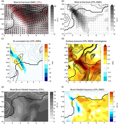
On 23rd at 00 UTC, another mechanism is at play (Fig. 8). This time, weak winds are present on the western side of the convergence zone with weak stratification. On the eastern side, south-southeasterly winds get a stronger easterly component in CPL than in SMO and the convergence zone moves to the west, where winds were weaker in SMO: rain is enhanced on the western side (+8 mm) and reduced on the eastern side (−10 mm). Again, a pressure anomaly is present in the convergence zone. However, the pressure gradient induced by it is located two grid-points further to the north-east than the observed wind anomaly (Fig. 8b and d). Thus, the pressure anomaly does not seem to play as large a role as on 22nd. This time, the wind changes could be linked to changes in stratification. In fact, the convergence zone limits an area of less stratified air (below 12×10⁻³s⁻¹) on the west to more stratified air on the east (over 12×10⁻³s⁻¹) in CPL (Fig. 8e). This spatial difference in stratification is larger in CPL than in SMO (Fig. 8f). Thus, a more stratified mass of air coming from the east encounters a less stratified mass of air on the west and penetrates more into the less stratified zone, moving the convergence zone to the west. A similar mechanism had been found in the case of 19 September 1996 too (Berthou et al., 2014).

Fig. 8 Same figure as Fig. 7 on 23 September 1994 at 00 UTC.

Pressure anomalies in the convergence zone, changes in stratification leading to changes in the blocking by the Alps or to a move of the convergence zone are three mechanisms that cause changes in precipitations. They all originate from the surface flux differences that occurred both in the Gulf of Lions and in the upstream zones. Therefore, they depend on the integrated flux difference under the wind trajectory in the boundary layer [also shown in Lebeaupin et al. (2006)]. Since the low-level jet has a similar intensity in both simulations except very locally in the convergence zones, the averaged flux differences on the wind path mainly depend on the SST differences of the different simulations.

4. Rain sensitivity to the SST

4.1. Constructing an index

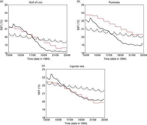
The presence of a convergence zone makes the precipitation events sensitive to anomalies in the SST field. However, this is not enough to build an index that could relate precipitation differences to SST differences. In fact, CPL-CTL also shows SST anomalies but very similar precipitation amounts. Figure 9b shows the SST evolution of the three simulations before the HPE on average in the three zones defined in Fig. 4c. The CPL simulation is colder than the SMO simulation in all the boxes during the 22–23 September event. Thus, the whole region upstream of the convergence zone is subject to weaker fluxes in CPL compared to SMO due to the smoothing of the Mistral event in SMO (Fig. 9c). In another way, the main anomaly between CPL and CTL simulations is located in the Pyrenees region (Fig. 4c). Figure 9b shows that the zone underwent a similar cooling in CTL as in CPL but with a persistent bias in SST which is not due to the last Tramontane/Mistral event. The atmospheric situation during the 2 d persists so that no air is advected from this zone to the convergence zone as shown in Fig. 7a and 8a. Therefore, no temperature anomaly is advected towards the convergence zone and the SST anomaly has no influence on it. Thus, the presence of precipitation anomalies depends on the position of SST anomalies that have to be on the trajectory of the air flowing towards the convergence zone. In this case, the upstream zones are thus the Gulf of Lions and the northeastern zones of the western Mediterranean basin.

Fig. 9 SST (°C) averaged over the boxes presented in Fig. 4c: (a) box (GoL); (b) box (Py); (c) box (Li). CPL (black plain line), SMO (black dashed line), CTL (red dashed line).

An index that takes into account both the intensity of the SST anomalies on the main wind trajectory and the presence of convergence can thus be developed to link precipitation differences to SST differences. Named IPSS for Index of Precipitation Sensitivity to the SST, it can be expressed as follows:1

where the first factor is the ratio between the surface area of the convergence zone () where and the total surface (), only considering the Gulf of Lions sub-domain (Fig. 4c). It shows whether there is a convergence zone before the air flows up onto the Cévennes and how spread it is. The second factor of the index is a spatial average of the squared SST anomalies (δSST _CPL-CTL or δSST _CPL-SMO ) over one or any combination of the regions (Reg) defined in Fig. 1:

• the Gulf of Lions (GoL)

• the zone offshore of the Pyrenees (Py)

• the Ligurian Sea extended down to North Sardinia (Li)

• a zone between the Balearic Islands and Sardinia (South Med)

• a zone between the Spanish coast and the Balearic Islands (Ba)

• the Tyrrhenian Sea (Ty)

Those zones are potential upstream zones for HPEs and can thus be important for the impact of SST changes on precipitation. The choice of the zones will be discussed later.

This index is calculated at every time step (3 h) and averaged over the day when the HPE was reported. It is expected that the higher the index, the larger the precipitation difference in HPEs between two simulations with different SST. This index can be applied to investigate both the effects of the submonthly coupling (CPL vs. SMO) or the effects of a different SST (CPL vs. CTL).

4.2. Test of the IPSS on the 22 most extreme HPE between 1989 and 2009

The IPSS was compiled on the 22 most extreme precipitation events in the Cévennes that occurred in the simulations run from 1989 to 2009. Those events were chosen for their daily accumulated precipitation amount larger than 110 mm in at least one grid point in CTL simulation in the Cvn box (Fig. 6a). Twenty-five days came out of this selection. However, three events lasted 2 d so we selected the most extreme of the 2 d to preserve the statistical independence of the selected events. They are presented in Supplementary Table 1. All the events are recorded as HPE by raingauge networks [Colin (2012), annex D; Ricard et al. (2012)] except 24 November 1993 and 27 October 1991. If we also take the 22 most extreme events in the rain analysis SAFRAN, we have to use a threshold of 190 mm and we get a hit rate for the model of 40% [as defined in Federico et al. (2008)]. In conclusion, 90% of the events of the simulation are heavy rain events recorded in the literature and 40% of them are among the most extreme events in reality. The event that occurred on 12–13 November 1999 studied by Lebeaupin Brossier et al. (2013) is also represented in this sample. An index showing the amount of precipitation difference between two simulations (I _rain) is calculated in the following way:2

Figure 10 shows the results for CPL vs. CTL index and CPL vs. SMO index with the average in SST anomalies taken in GoL and Li only since they were the upstream regions for our case study. The two sets of data share the extent of the convergence but show different intensities of SST differences. Thus, their IPSS is different. For example, in the case of 23 September 1994, the IPSS is 0.56°C for the difference CPL-SMO with an index of precipitation difference of 13.3 mm (Fig. 10 and Supplementary Table 1). For CPL-CTL, the IPSS is 0.38°C and the index of precipitation difference is 6.2 mm. The index shows a good relation between SST differences and the intensity of the precipitation difference for this case, where the upstream regions were Li and GoL. The case studied in Berthou et al. (2014) (19 September 1996) shows weaker precipitation differences for CPL-SMO for weaker IPSS and larger precipitation differences for CPL-CTL for a larger IPSS (Fig. 10 and Supplementary Table 1). This is in accordance with the hypothesis that precipitation differences are larger when the IPSS is larger. However, the case of 1996 shows very large precipitation differences for a moderate IPSS. This may be due to the particular sequence of that case that led to the build-up of an intense pressure anomaly located next to the convergence: this is a different mechanism than the simple vertical accumulation of temperature anomalies (Berthou et al., 2014). The case studied by Lebeaupin Brossier et al. (2013) (12–13 November 1999) shows precipitation differences mainly due to biases (for CPL-CTL, I _rain is 14.3 mm and IPSS is 0.74°C for 12th) since submonthly coupling effects shown by CPL-SMO are weaker (I _rain is 6.4 mm and IPSS is 0.27°C, Fig. 10 and Supplementary Table 1).

Fig. 10 Index of the precipitation difference (I _rain) (mm) as a function of the coupling index IPSS (°C) for the 22 strongest events represented by the model in the Cévennes area. Each event is represented by one red and one blue cross: red crosses represent the calculation of I _rain and IPSS for CPL-SMO and blue crosses for CPL-CTL. Moreover, three cases among the 22 are highlighted: squares show the case of 23 September 1994, discs show the case of 19 September 1996 and stars show the case of 12 November 1999.

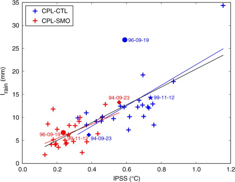
Table 1. Coefficient of correlation calculated between I _rain and IPSS (°C) with IPSS calculated on different regions indicated on the third line of the table and defined in Fig. 1

R value for
IPSS	IPSS	IPSS	IPSS	IPSS	IPSS	IPSS
GoL+Li	GoL+Co+Py	GoL	South Med	Ty	Ba	GoL+Li, no conv
CPL-CTL	0.66	0.64	0.60	0.51	−0.09	0.33	0.63
CPL-SMO	0.56	0.52	0.54	0.41	0.52	0.48	0.62
Both	0.76	0.75	0.73	0.65	0.43	0.61	0.74

Statistically significant coefficients of correlation above 99% are indicated with bold font.

The coefficient of correlation between I _rain , the index of precipitation difference and the IPSS is 0.56 for the CPL-SMO points and 0.66 for the CPL-CTL cloud of points. If all the points are taken into account, the coefficient of correlation is 0.76. These results show that I _rain and IPSS are well correlated independently from the time-scale of the SST differences (long-term biases or submonthly coupling). All these coefficients of correlation are significant above 99.5% using the Student t-test for the Pearson coefficient. This index is thus successful in showing how much change in precipitation can be generated by either biases in the SST (CPL-CTL) or by submonthly air–sea coupling during a HPE (CPL-SMO). It is interesting to note that SST differences are generally more important between CPL and CTL and lead to larger precipitation differences than those only due to submonthly coupling. This is why the coefficient of correlation using both sets is improved compared to only one set of data.

To test the sensitivity of the calculation of the IPSS to the definition of the zones, it was compiled with SST averages on different zones and the obtained coefficients of correlation are shown in Table 1. The first one (IPSS GoL+Li) corresponds to the one discussed above and shown on Fig. 10. Adding the Pyrenees to the area or taking the Gulf of Lions alone does not change the index much.

Thus, the index is robust when the box definition within the north-western Mediterranean is changed. If the IPSS is calculated either with the Ty, Ba or South Med (see Fig. 1), the coefficient of correlation gets worse (Table 1). Thus, the SST of remote zones shows less influence on the precipitation event: this confirms the analysis of the case studies. Finally, if the IPSS is computed without the factor of convergence, the regression coefficient does not change much. In fact, convergence is always present at some stage during the day in these HPEs reproduced by the model: it does not discriminate between those events. However, it may be useful for comparison of the effect on precipitations that are less intense and involve less convergence.

Therefore, the coefficient of correlation between I _rain and IPSS is quite robust to variations in its definition which makes it reliable. Moreover, the fact that the coefficient of correlation is higher with areas closer to the precipitation event makes us confident in the analyses of the case studies of 23 September 1994 and of Berthou et al. (2014) which showed atmospheric mechanisms that linked SST anomalies just upstream of the precipitation event with precipitation anomalies. Heavy rain events are subject to modulation of their rain amount that is proportional to the IPSS, which mainly reflects the mean SST differences from the Pyrenees to Corsica.

The IPSS calculated for CPL-SMO can be compared with the IPSS calculated between GOS-SST and GOS-SST smoothed over a month (with the convergence calculated using CPL simulation). This can show how good the representation of submonthly coupled effects is in CPL. For the case study of 23 September 1994, the IPSS_CPL-SMO is equal to 0.56°C when the IPSS_GOS-GOSsmo is 0.41°C. For the 19 September 1996, they are respectively 0.24°C and 0.26°C and for 12 November 1999 they are 0.27°C and 0.42°C. The mean value of the difference between the two IPSS over the 22 events is −0.03°C with a mean absolute error of 0.08°C and the coefficient of correlation between both indexes is 0.65. This shows that the CPL simulation represents quite well the submonthly coupled effects over this set of events. Thus, our conclusion that submonthly air–sea coupling can modulate heavy rain events (for strong IPSS) is strengthened by the good value of the IPSS in the model. If the relation between I _rain and IPSS is verified in other models, the IPSS calculated between GOS-SST and a smoothed GOS-SST could be used to assess the impact of coupled processes on the intensity of precipitation in real cases thanks to the calculated regression.

5. Conclusion

This case study completes previous studies from Lebeaupin Brossier et al. (2013) and Berthou et al. (2014) that showed precipitation differences linked with changes in SST. In fact, Lebeaupin Brossier et al. (2013) investigated the difference between CPL and CTL simulations but could not separate the precipitation differences coming from submonthly coupling effects such as the Mistral event that occurred 4 d before the event from the climatological differences between ERA-interim SST (CTL) and the SST calculated by the ocean model NEMO coupled to the atmospheric model WRF (CPL) in simulations running from 1989 to 2009. In Berthou et al. (2014), both effects were analysed separately and submonthly coupled effects were weaker than effects from the biases on the case study of 19 September 1996. However, the study highlighted atmospheric mechanisms that link SST anomalies to precipitation anomalies.

The present study shows that these mechanisms are also at play in the case of 22–23 September 1994, when SST differences originate from an intense Tramontane and Mistral event that started 10 d before the event and lasted 6 d. This event cooled the SST of the whole north-western Mediterranean by about 2°C with a larger impact on the French Riviera. In the SMO simulation, the decrease in SST is about half of this intensity since the SST gradually decreases with the monthly trend. Representing the sharp decrease of SST caused by the Mistral event thus brings a large temperature anomaly that leads to a precipitation decrease of 40 mm on a total of 220 mm in 2 d. The change in wind induced by SST differences is the main explanation for such a decrease with changes in stratification that cause a larger blocking and weaker convergence, to stratification changes that lead to a shift of the convergence zone and to pressure anomalies that are generated in the convergence zones.

Based on these findings, the Index of Precipitation Sensitivity to the SST (IPSS) was built to link SST differences to precipitation differences. It takes into account the extent of the convergence just upstream of the Cévennes in the Gulf of Lions and the extent of SST differences in the northwestern Mediterranean. It shows strong statistical significance when it is tested on the most extreme precipitation events that occurred between 1989 and 2009: the larger the IPSS, the larger the precipitation differences. The index is robust when different upstream regions are tested. Although the IPSS is computed with information about convergence, this factor is common to all HPEs reported by those simulations and is thus not a discriminating factor among them. The strong correlation between rain differences and IPSS shows that the SST in the zone from the Pyrenees to Corsica through the Gulf of Lion is one of the factors influencing the location and intensity of HPE located in the Cévennes through the influence of SST on the location of the convergence of low-level moisture. Moreover, the effect of submonthly variations of SST on HPE is lower than the effect of climatological biases between CPL and CTL but is still present: five events out of 22 reach rain differences higher than 9 mm averaged on the Cévennes (Fig. 10). Representing the submonthly variations of SST due to air–sea coupling has an impact on rain that is all the more important because the SST variations caused by the mistral/tramontane are large. In fact, in this region and for this season, submonthly coupled effects are mostly linked to Mistral/Tramontane events that lead to strong air–sea interactions. Submonthly variations of SST in the CPLs seem realistic compared with high resolution reanalyses. This validates the IPSS calculated with the CPL and SMO simulations.

The index developed in this study can further be used to assess the impact of submonthly coupled effects on HPEs in a CPL that has no equivalent of our SMO simulation. Indeed, the IPSS can be calculated by smoothing the SST of the ocean model and using the obtained regression. The index could also be tested on other regions where convergence initiates HPEs.

This study uses only one configuration of RCM and AORCM and the intensity of the response of the model to SST differences may be different owing to model differences. Thus, future work will use this index and compute the precipitation differences with similar twin simulations run within the Med-CORDEX program by different groups using different regional models to investigate the relation between SST changes and precipitation changes. If the relation is verified in other models, the index will also be useful for assessing the influence of submonthly coupled effect on precipitation events using high-resolution SST reanalyses and HyMeX data.

6. Acknowledgements

This work is a contribution to the HyMeX program (HYdrological cycle in The Mediterranean EXperiment) through INSU-MISTRALS support and the Med-CORDEX program (COordinated Regional climate Downscaling EXperiment Mediterranean region). This research has received funding from the French National Research Agency (ANR) project REMEMBER (contract ANR-12-SENV-001). It was supported by the IPSL group for regional climate and environmental studies, with granted access to the HPC resources of IDRIS (under allocation i2011010227). The authors acknowledge Météo-France who provided the situation description of the 22–23 September 1994 case and observation data (http://pluiesextremes.meteo.fr). We thank the Gruppo di Oceanografia da Satellite team (GOS), http://gos.ifa.rm.cnr.it/index.php, and MYOCEAN project for providing the GOS-SST product.

The authors are very grateful to Robert Jones for his corrections of the English text and to Bénédicte Jourdier for her help with graphism. We thank the anonymous reviewers for their help to improve the manuscript.

Notes

To access the supplementary material to this article, please see Supplementary files under Article Tools online.

References

- Béranger K. , Drillet Y. , Houssais M.-N. , Testor P. , Bourdallé-Badie R. , co-authors . Impact of the spatial distribution of the atmospheric forcing on water mass formation in the Mediterranean Sea. J. Geophys. Res. Oceans. 2010; 115(C12): C12041.
- Berthou S. , Mailler S. , Drobinski P. , Arsouze T. , Bastin S. , co-authors . Sensitivity of an intense rain event between an atmosphere-only and an atmosphere-ocean regional coupled model: 19 September 1996. Q. J. Roy. Meteorol. Soc. 2014
- Beuvier J. , Béranger K. , Lebeaupin Brossier C. , Somot S. , Sevault F. , co-authors . Spreading of the western Mediterranean deep water after winter 2005: time scales and deep cyclone transport. J. Geophys. Res. 2012; 117: 26.
- Beuvier J. , Sevault F. , Herrmann M. , Kontoyiannis H. , Ludwig W. , co-authors . Modeling the Mediterranean Sea interannual variability during 1961–2000: focus on the Eastern Mediterranean transient. J. Geophys. Res. Oceans. 2010; 115(C8): C08017.
- Brankart J. , Brasseur P . The general circulation in the Mediterranean Sea: a climatological approach. J. Mar. Syst. 1998; 18(1–3): 41–70.
- Colin J . Étude des événements précipitants intenses en Méditerranée: approche par la modélisation climatique régionale. [Study of intense precipitation events in the Mediterranean using regional climatic modelisation]. . 2012. PhD Thesis, CNRM-GAME, Météo France.
- Drobinski P. , Anav A. , Lebeaupin Brossier C. , Samson G. , Stéfanon M. , co-authors . Model of the regional coupled earth system (MORCE): application to process and climate studies in vulnerable regions. Environ. Model. Software. 2012; 35: 1–18.
- Drobinski P. , Bastin S. , Gunard V. , Caccia J. , Dabas A. , co-authors . Summer mistral at the exit of the Rhone valley. Q. J. Roy. Meteorol. Soc. 2005; 131: 353–375.
- Drobinski P. , Ducrocq V. , Alpert P. , Anagnostou E. , Béranger K. , co-authors . HyMeX, a 10-year multidisciplinary program on the Mediterranean water cycle. Bull. Am. Meteorol. Soc. 2014; 95: 1063–1082.
- Drobinski P. , Flamant C. , Dusek J. , Flamant P. , Pelon J . Observational evidence and modelling of an internal hydraulic jump at the atmospheric boundary layer top during a tramontane event. Boundary Layer Meteorol. 2001; 98: 497–515.
- Ducrocq V. , Nuissier O. , Ricard D. , Lebeaupin C. , Thouvenin T . A numerical study of three catastrophic precipitating events over southern France. II: Mesoscale triggering and stationarity factors. Q. J. Roy. Meteorol. Soc. 2008; 134(630): 131–145.
- Duffourg F. , Ducrocq V . Origin of the moisture feeding the heavy precipitating systems over southeastern France. NHESS. 2011; 11(4): 1163–1178.
- Federico S. , Avolio E. , Bellecci C. , Lavagnini A. , Colacino M. , co-authors . Numerical analysis of an intense rainstorm occurred in southern Italy. NHESS. 2008; 8: 19–35.
- Fusco G. , Manzella G. M. R. , Cruzado A. , Gačić M. , Gasparini G. P. , co-authors . Variability of mesoscale features in the Mediterranean Sea from XBT data analysis. Ann. Geophys. 2003; 21(1): 21–32. Copernicus GmbH.
- Giorgi F. , Jones C. , Asrar G. R . Addressing climate information needs at the regional level: the CORDEX framework. WMO Bull. 2009; 58(3): 175.
- Guénard V. , Drobinski P. , Caccia J. , Campistron B. , Bénech B . An observational study of the mesoscale mistral dynamics. Boundary Layer Meteorol. 2005; 115: 263–288.
- Guénard V. , Drobinski P. , Caccia J. , Tedeschi G. , Currier P . Dynamics of the map iop-15 severe mistral event: observations and high-resolution numerical simulations. Q. J. Roy. Meteorol. Soc. 2006; 132: 757–778.
- Homar V. , Romero R. , Ramis C. , Alonso S . Numerical study of the October 2000 torrential precipitation event over eastern Spain: analysis of the synoptic-scale stationarity. Ann. Geophys. 2002; 20: 2047–2066.
- Kain J. S . The KainFritsch convective parameterization: an update. J. Appl. Meteorol. 2004; 43(1): 170–181.
- Lebeaupin C. , Ducrocq V. , Giordani H . Sensitivity of torrential rain events to the sea surface temperature based on high-resolution numerical forecasts. J. Geophys. Res. Atmos. 2006; 111(D12): D12110.
- Lebeaupin Brossier C. , Béranger K. , Deltel C. , Drobinski P . The Mediterranean response to different spacetime resolution atmospheric forcings using perpetual mode sensitivity simulations. Ocean Model. 2011; 36(1–2): 1–25.
- Lebeaupin Brossier C. , Drobinski P . Numerical high-resolution air–sea coupling over the gulf of lions during two tramontane/mistral events. J. Geophys. Res. 2009; 114(D10): D10110.
- Lebeaupin Brossier C. , Drobinski P. , Béranger K. , Bastin S. , Orain F . Ocean memory effect on the dynamics of coastal heavy precipitation preceded by a mistral event in the northwestern Mediterranean. Q. J. Roy. Meteorol. Soc. 2013; 139: 1583–1897.
- Levitus S. , Antonov J. , Boyer T . Warming of the world ocean, 1955–2003. Geophys. Res. Lett. 2005; 32(2): L02604.
- Madec G. , Lott F. , Delecluse P. , Crpon M . Large-scale preconditioning of deep-water formation in the northwestern Mediterranean Sea. J. Phys. Oceanogr. 1996; 26: 1393–1408.
- Madec G. , The NEMO Team . NEMO Ocean Engine. 2008. Note du Pole de modélisation, Institut Pierre-Simon Laplace (IPSL), Paris, France. No 27 ISSN No 1288–1619.
- Marshall J. , Schott F . Open-ocean convection: observations, theory, and models. Rev. Geophys. 1999; 37(1): 1–64.
- Marullo S. , Buongiorno Nardelli B. , Guarracino M. , Santoleri R . Observing the Mediterranean Sea from space: 21 years of pathfinder-AVHRR sea surface temperatures (1985 to 2005): re-analysis and validation. Ocean Sci. 2007; 3(2): 299–310.
- Millán M. , Estrela M. J. , Caselles V . Torrential precipitations on the Spanish east coast: the role of the Mediterranean Sea surface temperature. Atmos. Res. 1995; 36(1): 1–16.
- Noh Y. , Cheon W. G. , Hong S. Y. , Raasch S . Improvement of the k-profile model for the planetary boundary layer based on large eddy simulation data. Boundary Layer Meteorol. 2003; 107(2): 401–427.
- Nuissier O. , Ducrocq V. , Ricard D. , Lebeaupin C. , Anquetin S . A numerical study of three catastrophic precipitating events over southern France. I: Numerical framework and synoptic ingredients. Q. J. Roy. Meteorol. Soc. 2008; 134(630): 111–130.
- Omrani H. , Drobinski P. , Dubos T . Optimal nudging strategies in regional climate modelling: investigation in a big-brother experiment over the European and Mediterranean regions. Clim. Dynam. 2013; 41: 2451–2470.
- Pastor F. , Estrela M. J. , Pearrocha D. , Milln M. M . Torrential rains on the Spanish Mediterranean coast: modelling the effects of the sea surface temperature. J. Appl. Meteorol. 2001; 40(7): 1180–1195.
- Quintana-Seguí P. , Le Moigne P. , Durand Y. , Martin E. , Habets F. , co-authors . Analysis of near-surface atmospheric variables: validation of the SAFRAN analysis over France. J. Appl. Meteorol. Climatol. 2008; 47(1): 92–107.
- Rajczak J. , Pall P. , Schär C . Projections of extreme precipitation events in regional climate simulations for Europe and the Alpine Region. J. Geophys. Res. Atmos. 2013; 118: 3610–3626.
- RIC. L’évaluation préliminaire des risques d'inondation 2011 bassin Adour-Garonne – sous bassin du Lot. [Preliminary evaluation of flood risks in 2011 in the Adour-Garonne basin and Lot sub-basin]. . 2012. Technical Report, Direction régionale de l'Environnement, l'Aménagement et du Logement.
- Ricard D. , Ducrocq V. , Auger L . A climatology of the mesoscale environment associated with heavily precipitating events over a northwestern Mediterranean area. J. Appl. Meteorol. Climatol. 2012; 51(3): 468–488.
- Salameh T. , Drobinski P. , Dubos T . The effect of indiscriminate nudging time on large and small scales in regional climate modelling: application to the Mediterranean basin. Q. J. Roy. Meteorol. Soc. 2010; 136(646): 170182.
- Simmons A. , Uppala S. , Dee D. , Kobayashi S . New ECMWF reanalysis products from 1989 onwards. ECMWF Newsletter. 2007; 110: 25–35.
- Skamarock W. C. , Klemp J. B. , Dudhia J. , Gill D. O. , Barker D. M. , co-authors . A description of the advanced research WRF version 3. 2008. Technical Report, DTIC Document.
- Small R. , deSzoeke S. , Xie S. , OŃeill L. , Seo H. , co-authors . Air–sea interaction over ocean fronts and eddies. Dynam. Atmos. Oceans. 2008; 45: 3. 274–4. 319.
- Stauffer D. R. , Seaman N. L . Use of four-dimensional data assimilation in a limited-area mesoscale model. Part I: Experiments with synoptic-scale data. Mon. Weather Rev. 1990; 118(6): 1250–1277.
- Stull R. B . An Introduction to Boundary Layer Meteorology. 1994; London, UK: Kluwer.
- Valcke S . Oasis3 user guide (prism_ 2-5). CERFACS PRISM Support Initiative Rep. 2006; 3: 60.