The importance of using a high-resolution model to study the climate change on small islands: the Lesser Antilles case

Abstract

High-resolution climate change simulations over the Lesser Antilles are performed using the ALADIN-Climate regional climate model nested within the global model ARPEGE (Météo-France). Three sets of simulations are conducted at 10 km grid spacing for reference (1971–2000) and future climate (2071–2100) under two CMIP5 scenarios (RCP4.5 and RCP8.5). With the dynamical downscaling, islands of Lesser Antilles are considered as land by the model, whereas, for the driving model, there is only sea over the domain. Temperature and precipitation change are analysed on land and on sea separately. For temperature, the warming is greater on land than on sea, especially for the minimum daily temperature (3.2°C vs. 2.3°C for the RCP85 scenario). For precipitation, projections are less reliable because the seasonality is not well reproduced by the model. Nevertheless, simulations exhibit the fact that projections on land differ from one island to the other and disagree with those on sea notably during the wet season. This underlines the importance of the dynamical downscaling to study the climate on small islands. Statistical downscaling has been performed on the Guadeloupe Island to study changes in extreme precipitation indices. The projections provided by the regional climate model suggest an increase in extreme rainfall events: longer dry periods, a bigger annual total precipitation, more frequent very heavy daily precipitation and a stronger 1 d maximum precipitation, whereas for the driving Global Climate Model, these trends are less intense.

• climate change
• regional climate model
• RCP scenarios
• Lesser Antilles
• temperature
• precipitation

1. Introduction

General Circulation Models (GCMs) have been widely used to produce long-term predictions of future climate change scenarios. Their simulations provide a representation of a possible climate in the future at a global scale. That way, in the IPCC report (AR5), the CMIP5 experiment provided a bundle of scenarios, with a horizontal resolution of 150 km. For several years, climate researchers have underlined the fact that the low spatial resolutions of GCMs are too coarse to assess the climate impact on a local scale (Gao et al., 2006; Somot et al., 2006) and proposed to use a downscaling method. As a bridge of transforming coarse outputs to a finer resolution, downscaling techniques have been developed from two general approaches focusing on atmospheric physics and empirical statistics respectively, namely dynamical downscaling and statistical downscaling. The latter can be considered as a method for correcting the behaviour of the model with statistical methods (Duan and Mei, 2013). Regarding the former approach, two kinds of numerical regionalization (or downscaling) techniques have been developed by modellers to generate regional climate information. One can use high-resolution GCMs or limited area models (LAMs) nested in a GCM called further regional climate models (RCMs) like in Li et al. (2013).

In this way, the Coordinated Regional Climate Downscaling Experiments (CORDEX) project aims to refine the resolution by atmospheric models at 50 km resolution over large continental domains, driven by CMIP5 models at their lateral boundaries and through the sea surface temperature (sst) (Giorgi et al., 2009). In general, high resolution enables a better representation of orography allowing the discrimination between various climate types over the country, and a better reproduction of the climate and heavy precipitation (Déqué and Somot, 2008; Somot et al., 2008). Gao et al. (2008) show the importance of using a high-resolution model to study the change in climate where the topography is complex. Indeed, they illustrate the differences between projections of precipitation in China from the RCM and those from the driving GCM and show the RCM trends are in better agreement with observed changes.

In the particular case of small islands, which have been long identified as being among the most vulnerable to climate change and climate extremes (IPCC, 2007, 2012), the challenge is different. Indeed, with the CORDEX experiments (50 km horizontal resolution), no land grid-point is located in our area of interest (12–20°N and 64–56°W), that is to say, all islands of Lesser Antilles are considered as sea by models; Puerto Rico and Venezuela are the nearest land-points to the studied location (far from ~500 km). It is well known that, in this region, the proximity of land has a strong influence on precipitation (Smith et al., 2012). In order to represent most of Lesser Antilles islands in the model and to illustrate the influence of lands on projections, a dynamical downscaling has been performed using the ALADIN-Climate RCM nested within the global model ARPEGE (Météo-France). Compared to the PRECIS-Caribbean project (Taylor et al., 2013) for which the RCMs were run at a 25 km resolution, the simulations presented in this paper focus on Lesser Antilles with a 10 km resolution and the most recent IPCC emissions scenarios (AR5) have been used.

The paper is sectioned as follows. A short description of the RCM and simulations is provided in Section 2. This is followed by a basic validation of the model performances in Section 3. Section 4 presents the RCM projections for which land and sea points are analysed separately. A statistical downscaling is proposed to examine the projections of precipitation extreme indices in Section 5, and Section 6 presents a summary and discussion of the results.

2. Model, experiments and data

2.1. Model

The CNRM-CM5 model (Voldoire et al., 2011) is one of the contributors to CMIP5. Its sst has been used to drive, after subtraction of the monthly mean bias according to the ERA40 observation Fiorino (2004), a 50 km resolution version of the atmospheric component of CNRM-CM5, ARPEGE version 5 (Déqué, 2010). The ARPEGE simulations have been, in turn, used to provide lateral boundary conditions to its limited area version called ALADIN-Climate (Radu et al., 2008; Colin et al., 2010). In fact ALADIN-Climate and ARPEGE-Climate share exactly the same computer code and solve on different grids the same discretized equations. In this study, we use the latest version (V5.2) for which more details can be found at http://www.cnrm.meteo.fr/gmgec/arpege-climat/ARPCLI-V5.2/index.html.

2.2. Experiments

We carry out simulations over the West Indies (12–20°N and 64–56°W, see Fig. 1) with the LAM ALADIN-Climate at a 10 km horizontal resolution. At this fine scale, most islands of Lesser Antilles are considered as land in the Land/Sea mask of the model (see Table 1). There are 47 land points and 7128 sea points. Even though the complex orography of these islands is not reproduced by the elevation proposed by the model, the fine scale enables to have points with a high elevation, especially in Dominica. Note that the domain is not centred on islands, but shifted to the East to capture the Atlantic influences which modulate the underlying climatology in the studied location.

Fig. 1 The box shows the ALADIN domain (12–20°N and 56–64°W: 850 km×850 km).

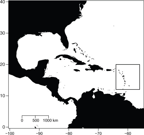
Table 1. For each island considered as land by ALADIN: area, highest elevation for ALADIN, CRU and Shuttle Radar Topography Mission (SRTM) and the number of land points in the grid of ALADIN and CRU

Highest elevation (m)			Number of land point
Island	Area (km^2)	ALADIN	CRU2.0	SRTM	ALADIN	CRU2.0
Antigua	281	121	1	402	1	1
Montserrat	102	110	227	914	1	1
Guadeloupe	1443	567	461	1467	15	7
Marie-Galante	158	84	1	204	1	1
Dominica	750	1227	1	1447	6	4
Martinique	1128	240	280	1397	10	6
Saint Lucia	620	244	167	950	6	4
Saint Vincent	345	416	315	1234	2	2
Barbados	431	98	110	340	5	2

http://www2.jpl.nasa.gov/srtm/.

Two periods are simulated by ALADIN-Climate: the present day period 1971–2000 with observed GHG (greenhouse gases) concentrations (called further run HIST), and the future period of 2071–2100 with GHG forcing from the IPCC emission scenarios (AR5): RCP4.5 and RCP8.5 (Moss et al., 2010).

2.3. Data

The ERA-interim reanalysis provides monthly mean atmospheric variables from 1979 up to now, gridded at a 0.75° resolution (Dee et al., 2011). Here we use the 2 m temperature and precipitation of the 156 sea points in our domain for the 1979–2000 period.

In addition, the CRU2.0 dataset provides monthly means for the period centred on 1961–1990 gridded at 10 min resolution over land areas only (New et al., 2002). Here we use the precipitation and the mean temperature of 28 points in our domain. Because of the low station density and the topographic complexity, the error in estimating CRU2.0 monthly precipitation can stand locally between 20 and 40% in the studied location (New et al., 2002). Nevertheless, the annual cycle can be considered well represented by this dataset.

3. Model validation

The model validation consists of evaluating the model's ability to capture variability in the large-scale patterns over the whole domain. In this way, mean monthly precipitation or temperature coming from the run HIST is compared to observed data presented in Section 2.3.

Monthly means over the whole domain are estimated by the median of the monthly mean of each point. The land and sea points are distinguished to underline how the model can reproduce the interface between land and sea.

3.1. Precipitation

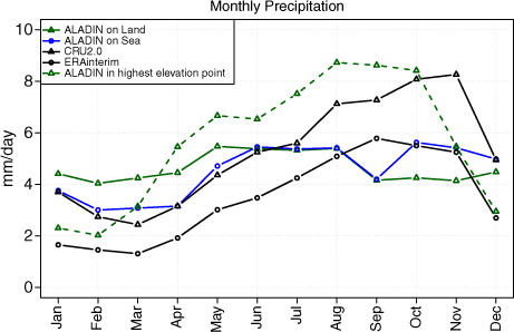
Figure 2 compares the monthly mean precipitation for ERA-interim, CRU 2.0 and run HIST of ALADIN-Climate. The ALADIN-Climate model demonstrates reasonable skill in reproducing the precipitation pattern between January and May even though the precipitation is overestimated: more precipitation on land than on sea, the peaking of the dry period in February and March. On sea, even though the seasonal variability is less marked by the model than observation, ALADIN-Climate reproduces well the annual cycle (except for September). However, the wet period (July–November) is generally not simulated by the model on land where the precipitation decreases from September. In fact, the model simulates the same precipitation amount for every month on land: the daily rainfall is not higher in the wet period. Nevertheless, there are some land points where the annual cycle is relatively well respected, especially on the highest elevation point (Dominica) where the seasonality and the intensity of wet days are well modelled by the ALADIN-Climate (see the dotted line in Fig. 2). For this island, ALADIN-Climate simulates with some success the seasonal variability. A possible explanation could be the relatively high elevation of this grid point which triggers seasonal convection more efficiently. However, there are not enough land points in this domain to check this hypothesis.

Fig. 2 Monthly mean precipitation over the area 12–20°N and 56–64°W, obtained from ERA-interim dataset in black with circles (median on 156 sea points), CRU2.0 dataset in black with triangles (median on 28 land points), ALADIN simulation on Land in green with triangles (median on 47 land points), ALADIN simulation on Sea in blue with circle (median on 7128 sea points) for the end of the 20th century. Units are in mm/day.

3.2. Temperature

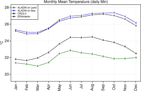
Figure 3 (resp. 4) compares the monthly mean of the maximum (resp. minimum) daily temperature for ERA-interim, CRU 2.0 and run HIST of ALADIN-Climate. Globally, the temperature is well represented by the model. On sea, the temperature proposed by the model is very similar to observation because of the subtraction of the monthly mean bias coming from the sst. On land, the model seems to underestimate the temperature (despite the application of a gradient of 0.0033 km⁻¹ to bring the temperature at the sea level). The seasonal variability is very well captured by the model, especially for the maximum daily temperature. In agreement with observation, the difference between Tmax and Tmin is more important on land than on sea (Fig. 4).

Fig. 3 Monthly mean Tmax (maximum daily temperature) over the area 12–20°N and 56–64°W, obtained from ERA-interim dataset in black with circles (median on 156 sea points), CRU2.0 dataset in black with triangles (median on 28 land points), ALADIN simulation on Land in green with triangles (median on 47 land points), ALADIN simulation on Sea in blue with circle (median on 7128 sea points) for the end of the 20th century. Units are in °C.

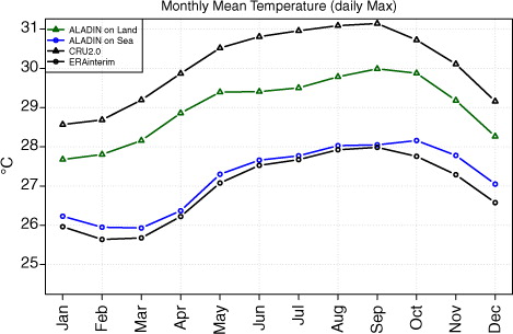
Fig. 4 Monthly mean Tmin (minimum daily temperature) over the area 12–20°N and 56–64°W, obtained from ERA-interim dataset in black with circles (median on 156 sea points), CRU2.0 dataset in black with triangles (median on 28 land points), ALADIN simulation on Land in green with triangles (median on 47 land points), ALADIN simulation on Sea in blue with circle (median on 7128 sea points) for the end of the 20th century. Units are in °C.

4. Projections

Projections under the RCP4.5 and RCP8.5 emission scenarios for the period 2071–2100 relative to the model baseline (1971–2000) are examined. RCP4.5 (resp. RCP8.5) temperature projections over the 21st century correspond approximately to those of SRES B1 (resp. A2-A1F1) (Rogelj et al., 2012).

Projections on land and sea are examined separately to underline the effect of land points on the RCM response. The significance of the changes in the monthly and annually values has been tested at a level risk α=0.05 for precipitation and temperature.

4.1. Temperature

First, for all model points and the two RCPs scenarios considered, temperatures increase significantly between 2000s and 2100s at a level significance α=0.05. Table 2 shows the anomalies of the monthly mean temperature (minimum and maximum daily) over the domain.

Table 2. Anomalies (median on all model points) of the monthly mean temperature between the period 1971–2000 and the period 2071–2100 according to the two scenarios (RCP4.5, RCP8.5)

Scenario	Model point	Jan	Feb	Mar	Apr	May	Jun	Jul	Aug	Sep	Oct	Nov	Dec	Year
Tmin	RCP4.5	Land	1.78	1.1	1.3	1.67	1.61	1.8	2.16	1.99	1.78	1.75	2.08	1.72	1.73
Sea	1.41	1.18	1.1	1.03	0.9	1.01	1.23	1.31	1.27	1.21	1.44	1.3	1.2
RCP8.5	Land	2.81	2.55	2.69	3.31	3.19	3.34	3.41	3.45	3.43	3.32	3.7	3.04	3.18
Sea	2.27	2.12	2.06	2.12	2.02	2.15	2.36	2.58	2.58	2.54	2.54	2.32	2.30
Tmax	RCP4.5	Land	1.58	1.45	1.47	1.46	1.43	1.36	1.4	1.48	1.45	1.4	1.52	1.53	1.46
Sea	1.43	1.18	1.06	0.97	0.85	1	1.23	1.32	1.28	1.18	1.43	1.32	1.19
RCP8.5	Land	2.66	2.52	2.66	2.73	2.57	2.54	2.66	2.88	2.93	2.9	2.84	2.75	2.72
Sea	2.28	2.13	2.03	2.09	1.98	2.16	2.36	2.58	2.58	2.53	2.51	2.34	2.30

All monthly mean temperature (min and max) increase significantly for all model points.

The RCM response is warmer (~+1.6°C/3.0°C) on land than on sea (~+1.2°C/2.3°C) for the RCP4.5/RCP8.5 scenario. Besides, compared to the sea points, the minimum daily temperature is generally more affected by the warming than the maximum temperature on land points.

Figure 5 shows, with a boxplot, the distribution of the anomalies of the seasonal temperature () on each island which are ordered from North to South. In addition, the Sea domain has been split in four zones (North–West, South–West, North–East, North–West) to appreciate if the changes are different on each zone. The RCM response is approximately the same in the whole Sea domain.

Fig. 5 Projections of the seasonal mean temperature for the period 2071–2100 relative to the period 1971–2000 baseline underline two scenarios (RCP4.5 in green and RCP8.5 in red) over all islands and Sea (divided in four zones: NW, NE, SE, SW). Units are in °C.

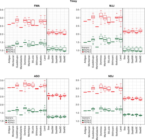
On land, the anomalies can be different from one island to another. For example, in the MJJ season, the temperature has an increase of 2.5°C for the RCP85 in Marie-Galante against 3.1°C for Dominica. Nevertheless, it seems there is no gradient North–South. The dry season FMA exhibits the lowest temperature response for Land and Sea.

4.2. Precipitation

Table 3 shows the proportion of model points for which the increase or decrease of the monthly mean precipitation is significant for each RCPs scenario. Sea and Land points are evaluated separately to underline the fact that future changes can be different on land and on sea. Indeed there are differences between projections on land and on sea. For example, under the RCP4.5 scenario, 69% of Land points have a significant increase for the mean precipitation in July, whereas 61% of Sea points have a significant decrease. It is approximately the same for June and September.

Table 3. Proportion of model points where the monthly mean precipitation increase (↗) or decrease (↘) significantly (at risk α=0.05) between the period 1971–2000 and the period 2071–2100 according to two scenarios (RCP4.5, RCP8.5)

Scenario	Trend	Model point	Jan	Feb	Mar	Apr	May	Jun	Jul	Aug	Sep	Oct	Nov	Dec	Year
RCP4.5	↗	Land	0	0	0	0	0	0.4	0.69	0.02	0.31	0	0.19	0	0.10
Sea	0.01	0	0	0	0	0	0	0	0	0	0.03	0	0
↘	Land	0.04	0.27	0.54	0.5	0.6	0.06	0.1	0.06	0.06	0.08	0	0.42	0.375
Sea	0	0.09	0.81	0.84	1	0.94	0.61	0.57	0.28	0.89	0	0.74	0.99
RCP8.5	↗	Land	0	0	0	0	0	0.4	0.6	0.1	0.15	0.02	0.33	0	0.02
Sea	0	0.01	0	0	0	0	0	0	0	0	0.01	0	0
↘	Land	0.62	0.48	0.94	0.52	0.42	0.08	0.02	0.02	0.1	0.6	0	0.71	0.56
Sea	0.75	0.22	0.89	0.61	0.98	0.63	0.74	0.7	0.78	0.86	0.07	0.94	0.99

The sea and the land points are analysed separately. Grey columns indicate months for which trends on land clearly differ from those on sea.

As for temperature, Fig. 6 shows projections of the seasonal mean precipitation for each island and each sea zone. On sea, seasonal rainfall is projected to decrease over the domain (~−15% for the two scenarios) and this decrease is generally more important in the South. No scenario seems to have a greater influence on precipitation projections on Sea.

Fig. 6 Projections of the seasonal mean precipitation for the period 2071–2100 relative to the period 1971–2000 baseline underline two scenarios (RCP4.5 in green and RCP8.5 in red) over all islands and Sea (divided in four zones: NW, NE, SE, SW). Units are in %.

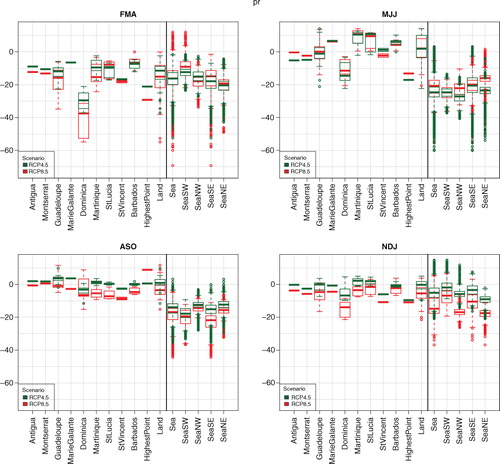
On land, precipitation decreases for the FMA season (dry season), but it is less important (~−10% for the RCP8.5 scenario) than on sea. The level of the drying varies with the island for which Dominica seems to have a drier response (~−40% for the RCP8.5 scenario) compared to the other. For the others seasons, no significant trend can be concluded. Globally the RCP8.5 scenario has a drier response than the RCP4.5 scenario on land for which the annual precipitation decreases significantly on the majority of grid points.

In the particular case of the highest elevation point on which the seasonal rainfall variability is well represented by ALADIN, monthly precipitation decreases significantly from January to June and December for both scenarios in agreement with projections on sea. Contrary to sea projections, a significant increase occurs in August (except for RCP4.5) and September. Figure 6 on which this particular point is noted HighestPoint, illustrates these opposite trends for the season ASO (wet period).

5. Statistical downscaling on Guadeloupe and projection of precipitation extreme indices

In this section, we illustrate the projections of some extreme indices concerning precipitation. As seen above, RCM simulations are not perfect reproductions of reality. Indeed, a comparison between observations and model output under reference condition has been made to highlight a model bias (see Section 3). This bias does not permit to estimate correctly the indices and so a correction has been made on the outputs model. Under the questionable, but implicitly admitted in IPCC-WG1 reports, assumption that the model bias stays the same under changing conditions, the same correction can be performed for both reference and future periods. In this paper, we focus on the Guadeloupe Island to show the link between anthropogenic emissions and impacts on extreme indices but this study can be extended to any island in our domain provided that daily observations are available.

5.1. Extremes indices

Some extreme indices are defined and described in detail in Klein Tank et al. (2009) and Zhang et al. (2011). All indices are calculated on each year to estimate the annual mean. Eleven indices which are recommended by ETCCDI to represent extreme precipitation are proposed:

1. cdd (consecutive dry days): count the largest number of consecutive days where the daily precipitation <1 mm,

2. cwd (consecutive wet days): count the largest number of consecutive days where the daily precipitation >1 mm,

3. rr1 (number of wet days): count the number of days where the daily precipitation >1 mm,

4. rr10 (number of very wet days): count the number of days where the daily precipitation >10 mm,

5. rr30 (number of heavy precipitation days): count the number of days where the daily precipitation >30 mm,

6. rr50 (number of very heavy precipitation days): count the number of days where the daily precipitation >50 mm,

7. cumul (total wet day precipitation): the amount of annual precipitation in mm,

8. sdii (simple daily intensity): the mean of the daily precipitation amount of wet days in mm,

9. r1d (max 1 d precipitation): The maximum of the daily precipitation in mm,

10. r3d (max 3 d precipitation): The maximum of the 3 d precipitation in mm,

11. r5d (max 5 d precipitation): The maximum of the 5 d precipitation in mm.

5.2. The model correction: q–q plot function

The model correction used here is the q–q plot method introduced by Déqué (2007). Using the q–q plot as a correction function is equivalent to consider that the RCM is able to predict a ranked category of precipitation but not a value for this variable. Thus, the goal is to transform the values simulated by the climate model in order to obtain a probability law near to the observation. The correction function is determined in comparing observations and the values of the climate model generated at the same period. The same function can then be applied to correct the simulated values under the different scenarios:

Let F be the cumulative distribution function (cdf) of the daily precipitation amounts generated by the RCM under the reference period 1971–2000 (run HIST).

Let G be the cdf of the daily precipitation amount of the observed data.

Let x be a daily precipitation generated by the RCM (for any scenario). Then the variable y corrected by the q–q plot method is defined by: y = G ⁻¹(F(x)).

From a practical point of view, we have a correction table with the 99 percentiles of the two distributions (reference simulation F and observation G) for each grid point or station. A linear interpolation is applied between two percentiles. Outside the table range, a constant correction is extrapolated.

5.3. Observations and the application of q–q plot correction

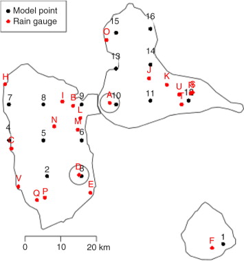
In Guadeloupe, 22 rain-gauge stations and 16 model points (see Fig. 7) are available to determine the cdf of the daily precipitation between 1971 and 2000. As seen above, the seasonal variability of precipitation is not well captured by the model. So the correction has been made month by month leading to determine 16×12F (from the run HIST) and 22×12G (from observation) which are empirically estimated by ~30×30 values.

Fig. 7 Twenty-two rain-gauge stations (daily precipitation) and the 16 land points of the RCM ALADIN-climate available in Guadeloupe.

Let F _(i,m) be the cdf of the daily precipitation simulated during the month m on the model point i (on the 1971–2000) and be the cdf the daily precipitation observed during the month mon the station s. Then the following steps are applied to determine the corrected daily precipitation of the three runs (HIST, RCP4.5 and RCP8.5):

for s=1 to22 (loop on stations) do

Let j the nearest land point model from station s

for m=1 to12 (loop on month) do

Let the daily precipitation simulated during the month m at the model point j,

Let , the daily precipitation of the model are corrected.

return

end for

end for

Thus, on each station, three series of daily precipitation are available for which the q–q plot correction has been made:

• on the period 1971–2000 (similar to observations) called run HISTcor

• on the period 2071–2100 under the RCP4.5 emission scenario called run RCP45cor

• on the period 2071–2100 under the RCP8.5 emission scenario called run RCP85cor

Table 4 illustrates the gains of the model correction on the calculation of extreme indices for two stations located by a circle in Fig. 7. For example, station A (altitude 11 m) which is associated with the model point 10 (altitude 56 m), is subject to an average of 3.9 daily rainfalls which exceed 50 mm per year between 1971 and 2000 (OBS) whereas, for the RCM, such a rainfall amount occurs only once in 30 yr (HIST). After the application of the q–q plot function (HISTcor), the number of very heavy rainfall is close to the reality. For all stations and all indices, the correction method permits to reproduce extreme precipitation very close to the reality. Note that the method does not correct the temporal properties of the series. Indeed, for station D (altitude 110 m) which is associated with the model point 3 (altitude 234 m), the max 1 d precipitation is well respected by HISTcor but the max 3 or 5 d precipitation is underestimated compared to observation.

Table 4. Comparison of precipitation extreme indices between observation and the output of the RCM at the nearest model point (before and after the q–q plot correction)

cdd	cwd	rr1	rr10	rr30	rr50	cumul	sdii	r1d	r3d	r5d
Station D	OBS	8.2	20.2	248.4	100.1	28.6	11.4	3425.1	13.8	138.1	223.2	280.7
HIST	6.5	30.9	278.3	41.0	0.33	0.07	1645.3	5.9	28.3	55.0	76.0
HISTcor	7.8	19.1	248.4	99.3	28.0	11.2	3419.7	13.8	138.1	192.7	244.0
Station A	OBS	13.4	11.0	176.3	44.4	10.4	3.9	1597.1	9.0	94.3	142.7	168.4
HIST	4.0	49.6	316.3	61.2	0.16	0.03	2123.1	6.7	24.1	46.7	67.4
HISTcor	12.5	10.5	176.4	44.3	10.5	4.4	1609.5	9.1	100.8	135.8	165.8

5.4. Projections of extreme indices after q–q plot correction

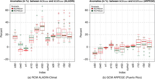
The projections (outputs for runs RCP45 and RCP85) are corrected in the same way than the run HIST to evaluate the possible changes in extreme precipitation under the two scenarios. Figure 8a illustrates the anomalies in percentage of each index between the present period (run HISTcor) and a possible future (run RCP45cor or run RCP85cor) from the corrected output of the RCM. Each boxplot is built from index calculated on 22 stations and provides information on the distribution of changes on Guadeloupe. Except for the cwd and rr1 indices for which the decrease is not really significant, all indices increase in the future for both scenarios. Even if the RCP8.5 scenario seems to have a bigger impact on extreme precipitation, both scenarios lead to similar results: longer dry period (~+2 d), a bigger annual total precipitation (~ +170 mm), very heavy daily precipitations more frequent (~+3per year) and a stronger 1 d maximum precipitation (~ +20 mm). These trends are in concordance with the observed trends illustrated in Stephenson et al. (2014).

Fig. 8 Anomalies of indexes between HISTcor and RCPcor in percentage.

It seems to have a contradiction between Table 3 (the annual cumul rather tends to decrease for land points) and Fig. 8a (annual cumul increases 20% for all points). But, this increase on corrected projections lies in the fact that there are a lot of land point where precipitation increases in June, July, September and November and that the q–q method permits to simulate heavier precipitation in wet seasons which determines, for the most part, the annual precipitation cumul while corrected precipitations during the dry season (FMA) which are in decrease have little influence on this cumul.

To illustrate the gains from high-resolution dynamical downscaling, RCM projections are compared to the GCM ARPEGE-Climate projections carried out at horizontal resolution 50 km. At this resolution, Puerto Rico is the nearest point considered as a land to Guadeloupe (~500 km). Even if this land point is far from Guadeloupe, this choice instead of a nearest sea point has been motivated by the fact that projections on sea points can be very different from land point projections, especially for precipitation (see Section 4). The same correction method has been applied to the Puerto Rico daily precipitation simulated by the ARPEGE-Climate GCM. Figure 8b illustrates the anomalies of indices between the present day and a possible future from the corrected GCM outputs and is to be compared with Fig. 8a. There are many opposite trends (cdd, rr30 and rr50), and when indices have the same trend (r1d, r3d and r5d), the GCM anomalies are smaller than RCMs.

6. Summary and discussion

The aim of this study was twofold: to present new climate simulations over Lesser Antilles under two CMIP5 scenarios and to underline the importance of using high-resolution models to examine the climate change on small islands.

High-resolution climate change simulations over Lesser Antilles are performed using the ALADIN-Climate RCM nested within the global model ARPEGE. Three sets of simulations were conducted at 10 km grid spacing for present day and future climate (2071–2100) under two CMIP5 scenarios (RCP4.5 and RCP8.5). With such a horizontal resolution, islands can be considered as land by the regional model whereas, for the driving model (50 km resolution), there is only sea over the domain and the nearest land grid points are situated at Puerto Rico or Venezuela.

For temperature, projections on sea and land are in the same way leading to a significant warming. Nevertheless, the presence of land grid points permits to underline the fact that this warming is more marked on land (~+1.6°C/3.0°C) than on sea (~+1.2°C/2.3°C) for the RCP4.5/RCP8.5 scenario. This fact shows that the dynamical downscaling which enables the inclusion of land points leads to notable advantages to examine the temperature change over small islands in a better way.

Contrary to temperatures for which ALADIN is capable of simulating the ‘present day’ annual cycle, the model has difficulties to reproduce precipitation well during the wet season, especially on land grid points. In fact, the RCM has difficulties to generate very heavy rainfalls which are common in a such location, especially during the wet season. This point is puzzling and leads us to consider uncertainties about the amount of precipitation changes. But, this weakness of the model should not mask the fact that the precipitation trends on sea can differ from those on land and, hence, the importance to have land grid points in a study of climate change. Climate models, through their complex equations, mimic reality, but their primary goal is not to reproduce it. These tools have been designed to explore the sensitivity to external factors like greenhouse gas, or the internal predictability from an observed initial state. Of course a good accuracy in representing present climate is always welcome, but it is not a proof that the mechanisms which lead to a different (future) climate are well described by the model equations. The recent development of decadal prediction will teach us how far bias and predictive skill are connected.

On sea, RCM projections show a decrease in annual precipitation (~ −20%) and are in agreement with those of the PRECIS project (Campbell et al., 2011). On land, RCM projections are moderate and can be different from one island to the other, but it seems that the RCM response tends to have wetter wet-seasons and drier dry-seasons. This difference between land and sea projections shows that the Sea/Land interface have a great importance to take into account the physical mechanisms caused by greenhouse gas change, and so the inclusion of land point is primordial to examine the model response to the precipitation change. The grid point where the precipitation is well reproduced has the same behaviour in terms of projections (drier dry-seasons and wetter wet-seasons) and enables us to argue the predicting capacity of the model even if it is globally not in agreement with the observation.

The RCM and the driving GCM projections on Guadeloupe are also compared in terms of extreme precipitation indices. For the driving model, the most suitable projections to study the climate change on Guadeloupe are those of Puerto Rico which is the nearest point considered as a land (~500 km). The same quantile–quantile correction method has been performed on the RCM and the driving GCM outputs in order to estimate the extreme indices close to observation. The RCM projections clearly show a trend in extreme precipitation indices: longer dry periods, a bigger annual total precipitation, very heavy daily precipitation more frequent and a stronger daily maximum precipitation, whereas for the driving model, these trends are weaker. These non-similar trends are not in contradiction, like in Gao et al. (2008), but only express different trends between Puerto Rico and Guadeloupe which can be explained by the different climate changes in these two locations.

Notwithstanding the previous arguments, the precipitation projections presented in the paper must be considered with caution, but underline the fact that high-resolution models, which include better resolutions of small islands, must be the starting point for future projections, for regions like the Caribbean, since land and sea are differently captured. A better representation of orography is a way to explore, in order to improve the model ability to capture the mean state, to bring relevance in the model results.

Finally, we present only the results of one RCM driven by one GCM. Comparison to our results with previous simulations (like PRECIS-Caribbean project) is difficult, as each simulation has a different scenario, model resolution and domain. Large ‘ensembles’ of simulations with different RCMs driven by different GCMs, possibly with an improved performance in simulating present day climate, are needed to increase the confidence in the projection of future climate over Lesser Antilles.

Notes

¹No land point is located on the domain.

²The thresholds of some indices are been changed to be adequate with the tropical climate.

³This simulation drive the ALADIN-Climate.

References

- Campbell J. D. , Taylor M. A. , Stephenson T. S. , Watson R. A. , Whyte F. S . Future climate of the Caribbean from a regional climate model. Int. J. Climatol. 2011; 31(12): 1866–1878.
- Colin J. , Déqué M. , Radu R. , Somot S . Sensitivity study of heavy precipitation in limited area model climate simulations: influence of the size of the domain and the use of the spectral nudging technique. Tellus A. 2010; 62(5): 591–604.
- Dee D. P. , Uppala S. M. , Simmons A. J. , Berrisford P. , Poli P. , co-authors . The era-interim reanalysis: configuration and performance of the data assimilation system. Q. J. Roy. Meteorol. Soc. 2011; 137(656): 553–597.
- Déqué M . Frequency of precipitation and temperature extremes over France in an anthropogenic scenario: model results and statistical correction according to observed values. Glob. Planet. Chang. 2007; 57(1–2): 16–26.
- Déqué M . Regional climate simulation with a mosaic of RCMs. Meteorol. Z. 2010; 19: 259–266.
- Déqué M. , Somot S . Analysis of heavy precipitation for France using ALADIN RCM simulations. Idojaras. 2008; 112: 179–190.
- Duan K. , Mei Y . A comparison study of three statistical downscaling methods and their model-averaging ensemble for precipitation downscaling in China. Theor. Appl. Climatol. 2013; 116: 1–13.
- Fiorino M . A Multi-Decadal Daily Sea Surface Temperature and Sea Ice Concentration Data Set for the Era-40 Reanalysis. 2004; 1–16. European Centre for Medium Range Weather Forecasts: ERA-40 Project Report Series, No. 12.
- Gao X. , Pal J. , Giorgi F . Projected changes in mean and extreme precipitation over the Mediterranean region from a high resolution double nested RCM simulation. Geophys. Res. Lett. 2006; 33(3): L03706.
- Gao X. , Shi Y. , Song R. , Giorgi F. , Wang Y. , co-authors . Reduction of future monsoon precipitation over China: comparison between a high resolution RCM simulation and the driving GCM. Meteorol. Atmos. Phys. 2008; 100: 73–86.
- Giorgi F. , Jones C. , Asrar G. R . Addressing climate information needs at the regional level: the CORDEX framework. World Meteorol. Organ. Bull. 2009; 58(3): 175.
- IPCC. Climate Change 2007: The Physical Science Basis, Contribution of Working Group I to the Fourth Assessment Report of the Intergovernmental Panel on Climate Change. 2007; Cambridge University Press, Cambridge, UK, New York, USA.
- Managing the Risks of Extreme Events and Disasters to Advance Climate Change Adaptation: A Special Report of Working Group I and II of the Intergovernmental Panel on Climate Change. Cambridge University Press. Online at: http://ipcc-wg2.gov/SREX/report/full-report/ .
- Klein Tank A. M. G. , Zwiers F. , Zhang X . Guidelines on analysis of extremes in a changing climate in support of informed decisions for adaptation. Climate data and monitoring WCDMP.
- Moss R. , Edmonds J. , Hibbard K. , Manning M. , Rose S. , co-authors . The next generation of scenarios for climate change research and assessment. Nature. 2010; 463(7282): 747–756. [PubMed Abstract].
- Li H. , Kanamitsu M. , Hong S.-Y. , Yoshimura K. , Cayan D. , co-authors . Projected climate change scenario over California by a regional ocean–atmosphere coupled model system. Clim. Chang. 2013; 122: 609–619.
- New M. , Lister D. , Hulme M. , Makin I . A high-resolution data set of surface climate over global land areas. Clim. Res. 2002; 21(1): 1–25.
- Radu R. , Déqué M. , Somot S . Spectral nudging in a spectral regional climate model. Tellus A. 2008; 60(5): 898–910.
- Rogelj J. , Meinshausen M. , Knutti R . Global warming under old and new scenarios using IPCC climate sensitivity range estimates. Nat. Clim. Chang. 2012; 2(4): 248–253.
- Smith R. , Minder J. , Nugent A. , Storelvmo T. , Kirshbaum D. , co-authors . Orographic precipitation in the tropics: the Dominica experiment. Bull. Am. Meteorol. Soc. 2012; 92: 1567–1579.
- Somot S. , Sevault F. , Déqué M . Transient climate change scenario simulation of the Mediterranean sea for the twenty-first century using a high-resolution ocean circulation model. Clim. Dyn. 2006; 27(7–8): 851–879.
- Somot S. , Sevault F. , Déqué M. , Crépon M . 21st century climate change scenario for the Mediterranean using a coupled atmosphere–ocean regional climate model. Glob. Planet. Chang. 2008; 63(2): 112–126.
- Stephenson T. S. , Vincent L. A. , Allen T. , Van Meerbeeck C. J. , McLean N. , co-authors . Changes in extreme temperature and precipitation in the Caribbean region, 1961–2010. Int. J. Climatol. 2014; 34: 2957–2971.
- Taylor M. A. , Centella A. , Charlery J. , Bezanilla A. , Campbell J. , co-authors . The PRECIS-Caribbean story: lessons and legacies. Bull. Am. Meteorol. Soc. 2013; 94(7): 1065–1073.
- Voldoire A. , Sanchez-Gomez E. , Salas y Mélia D. , Decharme B. , Cassou C. , co-authors . The CNRM-CM5.1 global climate model: description and basic evaluation. Clim. Dyn. 2011; 40: 2091–2121.
- Zhang X. , Alexander L. , Hegerl G. C. , Jones P. , Tank A. K. , co-authors . Indices for monitoring changes in extremes based on daily temperature and precipitation data. Wiley Interdiscipl. Rev Clim. Chang. 2011; 2(6): 851–870.