Representer-based variational data assimilation in a spectral element shallow water model on the cubed-sphere grid

Abstract

A representer-based variational data assimilation system is newly developed for the spectral element shallow water model in the High Order Method Modeling Environment. This study includes the development of tangent linear and adjoint codes and a background error covariance model. The correctness of the developed codes were checked by various ways such as linearity tests for tangent linear codes, adjoint tests for adjoint codes and symmetric tests for representer functions, which are four-dimensional covariance functions in observation-space. Then, direct and indirect representer-based data assimilation systems were constructed and evaluated by performing a series of identical twin experiments, where synthetic data were obtained from a reference run (nature run) and assimilated to correct initial conditions. The characteristics of the covariance model according to the different horizontal scales were evaluated by a suite of single-observation experiments. The results show satisfactory behaviours for both direct and indirect representer-based variational data assimilation methods, which indicates that they are ready to be further developed as a full-fledged four-dimensional variational data assimilation system as next step.

• Direct/indirect representer data assimilation
• spectral element shallow water model
• tangent linear model
• adjoint model
• background error covariance
• correctness test
• numerical weather prediction

1. Introduction

For the last two decades, variational data assimilation (DA) systems have been widely used for operational numerical weather prediction (NWP) systems (Rabier, 2005). Variational DA seeks to find minimisers of cost functions, which measure the misfit of model states from background and observations over given numerical domains and time intervals of interest. In general, the cost function is chosen as minus the logarithm of a probability density function. And, for Gaussian background and observational errors, the cost function is a weighted sum of squared residuals between data and model inputs such as initial conditions, boundary conditions and/or forcings. For the general case, the probability density function can be linearised so that the cost function can be taken as a quadratic form. A minimiser of a cost function is generally called an analysis field, which mathematically and statistically represents a best estimate of the current state in the model conditioned on given observations. Such analysis can be obtained by iterative minimisation algorithms, which require gradient information for a given cost function. In large dimensions, gradient information can be efficiently calculated from the adjoint model (ADM) of a forecast model.

Details of the design of each four-dimensional variational DA (4DVAR) system can be different from each other, for example, the model-space incremental 4DVAR in ECMWF (Rabier et al., 2000), the observation-space representer 4DVAR in NRL (Xu et al., 2005) and see Courtier (1997) for the duality between those two formulations. However, variational DA systems have the following main components in common: (1) tangent linear and adjoint codes of the forecast model, (2) tangent linear and ADMs of observation operators, (3) a background error covariance model and (4) iterative optimisation algorithms as a main driver of the variational DA system.

In this study, we developed representer-based 4DVAR systems (Bennett, 1992, 2002) for a global spectral element shallow water (SW) system (Taylor et al., 1997) adapted from the High Order Method Modeling Environment (HOMME, Dennis et al., 2005). Spectral element methods do not have pole problems since the sphere can be tiled with squares of approximately the same size, thus avoiding the clustering problem at the poles. By using a local coordinate system within each element, the problems of singularities in the coordinate system can be avoided, while it has a strong advantage of scalability for the future high performance computing environment. A numerical model that has similar characteristics of the grid structure and numerics is currently under development by the Korea Institute of Atmospheric Prediction Systems (KIAPS), funded by the Korea Meteorological Administration.

Before a 4DVAR system is fully developed for operational NWP and ocean forecasting, it is tested with comparatively simple systems such as global SW systems or double gyre ocean models (Courtier and Talagrand, 1990; Zhu et al., 1994; Xu and Daley, 2002; Moore et al., 2004; Kurapov et al., 2007). Xu and Daley (2002) investigated the cycling representer methods and formulated an accelerated representer algorithm with two-dimensional, multivariate barotropically unstable SW system. Moore et al. (2004) used a two-dimensional time evolving double gyre to test tangent linear, adjoint and various tools in the regional ocean modelling system (ROMS) before the 4DVAR system in ROMS were fully developed for a 3 dimensional ocean model. Also, Kurapov et al. (2007) tested a representer-based 4DVAR with a SW model and studied the circulation in a nearshore surf zone.

The objective of the current study is to develop all the utilities of 4DVAR based on direct and indirect representer methods, that is, tangent linear, its adjoint codes, and background covariance models, for a global spectral element SW system and to test the utilities with the isolated mountain test case of Williamson et al. (1992). The performance of the developed DA system is evaluated via a series of identical twin experiments. This study is focused on fundamental aspects of DA for a SW model, especially potential usage of representer-based 4DVAR systems for spectral element numerical methods, while addressing a next step toward development of a 4DVAR system for a three-dimensional primitive equation model.

In Section 2, the governing equations of the HOMME dynamical cores are explained. The development of tangent linear and its ADMs, and the background error covariance model is described in Sections 3, followed by a description of direct and indirect representer methods in Section 4. Section 5 presents the numerical results of single-observation experiments on the horizontal length scale effect in covariance models, and the results of identical twin experiments with the 4DVAR systems based on both direct and indirect representer methods. The summary and discussions are given in Section 6.

2. Dynamical model

The sphere is decomposed into six identical regions, using the central (gnomonic) projection of the faces of the inscribed cube onto the spherical surface (Sadourny, 1972; Ronchi et al., 1996; Nair et al., 2005). Figure 1a shows the surface of the cubed sphere that is the computational domain, where each cube face consists of an array of Ne×Ne spectral elements and each element contains Np×Np Gauss–Lobatto–Legendre (GLL) points. The non-overlapping faces are all singularity-free subdomains, and the discretisation is considered only for a single subdomain. The leapfrog trapezoidal method is used for time integration but for the first time step in HOMME, the forward Euler procedure was implemented with a half time step. It is because two digits of accuracy in the energy is lost without the procedure. See details of the numerical discretisation of space and time in Taylor et al. (1997) and Nair et al. (2005). The cubed-sphere grid with gnomonic projection is known as an excellent choice for high-order methods for global modelling applications like HOMME, the default dynamical core in the Community Atmosphere Model and the Community Earth System Model, which also solves a primitive hydrostatic equation using a spectral element method (Dennis et al., 2012).

Fig. 1 (a) The cubed-sphere computational domain with Gauss–Lobatto–Legendre (GLL) points of N _p ×N _p in the N _e elements, (b) zonally uniform flow over the isolated mountain at the initial time, (c) zonal wind field (contours, ms⁻¹) after 14-day time integration.

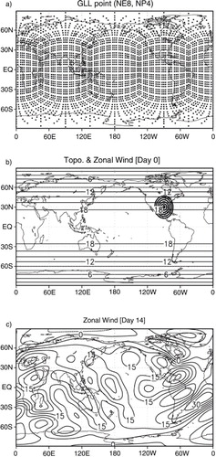
Here, we consider the SW model within HOMME for test case 5 in Williamson et al. (1992), zonal flow over an isolated mountain (Fig. 1b). The centre of the mountain is located at the numerical position with height m, where , , and λ and θ are, respectively, the longitudinal and latitudinal directions (Fig. 1b). The test case consists of solid body rotation and the Coriolis parameter that depends on latitude. The zonal wind flow is uniform over an isolated mountain at the initial time. The initial velocity field is (u, v)=(u ₀·cosθ, 0) with and a is the Earth radius. Figure 1c shows the zonal wind fields after 14-day time integration.

3. Utility development

Like other 4DVAR systems, the representer-based DA is also composed of a tangent linear model (TLM), its ADM, observational operators and a background error covariance model. There are different ways to develop those utilities. For example, the ADM code can be developed by directly discretising from the continuous adjoint equations or line-by-line coding from a perturbation forecast model, which is a linearised and then discretised form of the non-linear model (NLM). Lawless et al. (2003) defined the former as the continuous and the latter as the semi-continuous approaches to obtain an ADM. For simplicity, the ADM code in this study was written by a line-by-line transpose of the TLM, and both numerical codes in TLM and ADM are manually constructed following the recipes for adjoint coding as in Giering and Kaminski (1997) and Zou et al. (1997). It is worth noting that only this approach leads to consistent formulations of non-linear, tangent linear and adjoint code within machine precisions.

Symbolically, the non-linear SW forecast model could be written as a single evolution equation,1

The N is the NLM operator. The field x is the state vector [u, v, p] and the state variables (u, v) and p respectively are wind and geopotential fields in the HOMME SW model.

3.1. TLM and correctness checks

A correctness check of tangent linear codes is an essential part to test if they correctly present the tangential behaviour of a given non-linear code. Here two measures are evaluated as:2a 2b

where δx is the linear perturbation and M is a linear operator. Eq. (2a) states that for infinitesimal perturbations, the difference between the unperturbed and perturbed non-linear evolutions is expected to correspond to the tangent linear evolution. This relationship should hold within a machine precision as the magnitude of the scale factor α becomes small for the correctly developed tangent linear code. The other measure [eq. (2b)] not only compares the size of the non-linear (finite difference) and tangent linear evolution of the initial perturbations but also their vector difference.

Figure 2 shows that as the size of perturbation decreases, the tangent linear measure approaches to the ideal value, 1, within a machine precision. When the perturbation goes too small, however, the tangent linear measure gets worse due to the numerical round-off error, which is a general behaviour shown in the process of verifying the correctness of TLM. Figure 3 compares the 15-day evolved field of the TLM with the difference field of ‘perturbed’ and ‘unperturbed’ non-linear fields for meridional wind components. For this case, the initial perturbation δx is defined as 10% magnitude of initial field x (0)= x ₀ and α=10⁻². The two fields are well matched to each other with a pattern correlation coefficient higher than 0.98. Therefore, one can conclude that the TLM well represents the tangential dynamics for the given SW system in HOMME.

Fig. 2 Log of TL measures for (a) eq. (2a) and (b) eq. (2b) for each model state variable according to the scaling factor α. The vertical and horizontal axes are shown in logarithm scales.

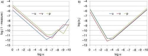
Fig. 3 Meridional wind fields after 15-day time evolution of the initial perturbation for (a) TLM and (b) difference of ‘perturbed’ and ‘unperturbed’ non-linear models. Contours are shown with 0.5 ms⁻¹ intervals without the zero contours.

3.2. Adjoint model and correctness checks

For the correctness of any adjoint code, it should satisfy the following adjoint relationship for a given tangent linear code within a machine precision:3

Adjoint codes are determined to be correctly developed if the self-inner product of the TLM with a given perturbation is the same as the inner product of the perturbation and the ADM of which the initial condition is the TLM result. This correctness check can be applied to any individual codes including time evolving modules. For adjointness checks, 1-day tangent linear integration and 1-day adjoint integration are performed. The evaluated adjoint measure in eq. (3) is 17389598702.128990 for the left-hand side and 17389598702.128815 for the right hand side. We attained 14 digits of accuracy. The results confirm the correctness of the developed ADM for the given TLM.

3.3. Representer matrix and symmetric tests

The overall correctness of a TLM and its ADM, given a forecast model including a non-linear observation operator H and the background covariance model P ^b , can be evaluated by a symmetry check of the q×q representer matrix R with q being the number of observations (Bennett, 2002). The representer matrix is defined as follows:4

Here, H and H ^T are respectively a tangent linear of observation (forward) operator and adjoint operator for H that links the model state to the observation. The i-th column of the q×q representer matrix can be explicitly constructed by sampling the measured values of the i-th representer function at q locations (see Section 4 for more details). For symmetric tests, the observation operator is set to be a simple bi-linear interpolation, and its corresponding adjoint module is also developed. And, the background error covariance is set to be an identity matrix (i.e. P ^b =I). Because the representer matrix must be symmetric (Bennett, 1992, 2002), off-diagonal components with respect to the main diagonal should be exactly same such that R−R ^T =0 within a machine precision. The result of the symmetric test showed that at least 13 digits of accuracy were attained, which indicates that the TLM and ADM of the NLM and the observation operator are correctly constructed.

3.4. Covariance model

A careful specification of the background error and the observation error covariances is a critical factor that directly influences the performance of a DA system (Daley, 1991). The background error covariance characterises the balance properties between state variables, spatial spreading of information, and smoothing of the increments (Bouttier and Courtier, 1999). Given a large dimensionality, however, the background error covariance cannot be explicitly constructed, while the observation error covariance is usually on the main diagonal (zero on the off-diagonal elements) with the given variances corresponding to the noise level in the data. The background error covariance P^b should be dealt with a covariance ‘model’, which is factorised as a series of matrices (Bannister, 2008a, 2008b):5

where K _b represents the balance properties between state variables and C represents the spatial correlation of unbalanced variables with the standard deviation Σ, which is diagonal. In this study, however, the geostrophic balance model developed and implemented for the spectral element SW model in HOMME is not yet considered for simplicity. Thus, the covariance model has simple univariate properties, partitioned as a squared-root of variances and spatial correlations:6

Note that since the cubed-sphere grid at the GLL node (and wind vector components in this coordinate) is not orthogonal, the transform matrix D is used to define the conventional zonal- and meridional wind components, which are orthogonal (Taylor et al., 1997):7

The background error covariance then can be constructed with the transform matrix D, its inverse matrix and the adjoint as follows:8

The climatological variance can be specified by several methods including the NMC (National Meteorological Center) method (Parrish and Derber, 1992), the observation method (Hollingsworth and Lonnberg, 1986) or ensemble-based methods (Fisher and Anderson, 2001). In our experiments below, we specified 1 m²s⁻² and 250 m⁴s⁻² variance values for wind and geopotential variables, respectively. The univariate spatial correlations are modelled by solving a pseudo-heat equation (Derber and Rosati, 1989; Weaver and Courtier, 2001), which has a similar effect to Gaussian filtering:9

with the Laplace operator ∇² and a constant diffusion coefficient κ. Because the product of the diffusion coefficient and the integration time determines the shape of the correlation function, the product keeps a constant. The correlation length scale will be investigated by changing the discrete time iteration Δτ in eq. (9) in order to characterise horizontal scales of the information spread in the single-observation experiment described in Section 5. Note that since the dynamical core is defined on cubed sphere, there is no pole problem that is usually shown in latitude–longitude grids.

4. Representer method

The representer-based DA scheme was first introduced in the field of oceanography (Bennett and McIntosh, 1982; Bennett and Thorburn, 1992). The representer method solves a linearised Euler–Lagrange equation by using its TLM and ADM of the corresponding NLM (Bennett, 1992, 2002; Chua and Bennett, 2001), and has been applied for ocean forecasting systems (Smith and Ngodock, 2008; Kurapov et al., 2009). Xu and Daley (2000) extended the representer method to the cycling representer method by establishing the theory and applications of the method in the field of meteorology (Ngodock et al., 2007). Then, Xu and Daley (2002) further extended the method to formulate the accelerated representer algorithms. Such extended algorithms are also implemented in three-dimensional primitive equations for operational NWP and ocean forecast systems (Xu et al., 2005; Rosmond and Xu, 2006; Ngodock et al., 2009; Chua et al., 2013).

In the theory of the calculus of variations, the minimiser of the cost function that measures the misfit between data and model results is obtained when the first variation is equal to zero, which can be formulated as Euler–Lagrange equations. The representer method approximates the solution to the Euler–Lagrange system with a sequence of solutions to linear problems such that10

where x _a and x _b are the analysis and background states and δx is an analysis increment. That is, the analysis is expressed by the sum of the background and the analysis increment, and the increment is obtained by a weighted (β _k ) linear combination of the representer functions γ _k , where k=1,…, q and q is the number of observations. Γ ^T β is a matrix expression for the weighted linear combination, and the weight β can be obtained by solving the following linear equation:11 12 13

where the vector y is observations, and O is an observational error covariance. Eqs. (12) and (13) show how to obtain the representer matrix R whose i-th column is the i-th representer function. Eq. (12) is thus called the backward or adjoint equation that yields the i-th adjoint state by integrating the ADM backwards in time with a forcing (or delta function) at the i-th observational location. With the initial condition of the i-th adjoint state applied by the background error covariance, eq. (13) yields the i-th representer function by integrating the TLM forward in time and then sampling the values at the i-th location.

For a direct calculation of the representer function for each observation, the matrix term of the left-hand side in eq. (11) can be explicitly constructed. For example, given the zonal wind observed at (35°W, 12.5°S) and at 3 hours from the initial time (black×in Fig. 4), the ADM is first integrated backwards in time with a forcing of the delta function. Figure 4a shows the structure of sensitivity at the initial time. The positive zonal wind sensitivity is mainly located in the upstream region from the observation, with cyclonic (anti-cyclonic) circulation to the northern (southern) region. Since the background error covariance P ^b shows only univariate correlation, multivariate correlations may be caused by the model constraints such as continuity, geostrophic balance and so on. By integrating TLM, the positive zonal perturbation fields are maximised in its original time and space (Fig. 4b), and then the perturbation fields are evolved to the downstream regions.

Fig. 4 Spreads of observational information with the colour shadings. (a) The structure of the initial sensitivity (time t=0) obtained by integrating ADM backwards in time and then by applying the covariance matrix P ^b in eq. (8). The zonal wind observation (×) is initially located at (35°W, 12.5°S) at 3 hour. Then, TLM is integrated with the initial sensitivity as the initial condition at time (b) 3, (c) 6, (d) 12, (e) 18 and (f) 24 hours, respectively. Arrows represent the wind vectors.

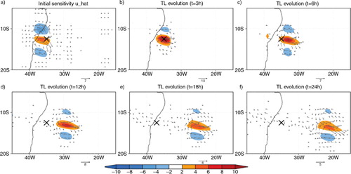
With the adjoint state applied by the covariance matrix P ^b in eq. (8) at the initial time, the TLM is evolved forward in time. That is, the ADM simulates the development of sensitivities backwards in time, the background error covariance P ^b in eq. (8) is applied to the adjoint state at the initial time, and the TLM simulates the development of perturbations with time (Holm, 2008; Moore, 2011). Then, the representer matrix R is constructed by sampling model values at the observational locations and times from the trajectories of the TLM. Therefore, the representer matrix represents a flow-dependent covariance for the multivariables, u, v and p within the assimilation window based on the (linear) model dynamics, and is a positive-definite, symmetric matrix. Since O is usually a diagonal matrix, R+O is also a positive-definite, symmetric matrix. Thus, the eq. (11) can be easily solved for β using a Cholesky factorisation. With the coefficient β , the analysis increment δx can be constructed with a linear combination of representer functions for observations. For a small number of observations, this algorithm is an effective way to solve a generalised inverse problem. For the case of many observations, however, the direct representer is computationally too expensive requiring one backward integration and one forward integration for each observation.

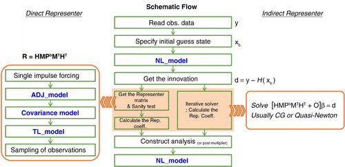
The indirect representer solves eq. (11) by using iterative solvers, which are usually conjugate-gradient or quasi-Newton algorithms. For a comparison of direct and indirect methods, see the schematic flow chart in Fig. 5. The indirect representer method does not require explicit construction of a full representer matrix, so it can be feasible even for a large number of observations. The solution of eq. (11) can be obtained iteratively by treating the multiplication by the inverse as a solution of the linear system, instead of computing the inverse of a matrix and multiplying by it. A standard iterative solver can convert a first-guess representer coefficient into a solution of the linear equation. The computationally intensive part of the iterative optimisation algorithms is mostly matrix–vector multiplication in the left-hand side in the eq. (11). There exist various efficient software packages to compute the iteration such as LAPACK on serial and shared memory computers and ScaLAPACK on distributed memory computers (Mandel, 2006).

Fig. 5 Schematic flow of direct and indirect representer algorithms (middle column). The direct method in the left column first constructs the representer matrix explicitly by directly applying a series of models such as ADM, covariance and TLM, and then the linear equation in eq. (11) is solved for the representer coefficients β. The indirect method in the right column approximates the representer coefficients in eq. (11) by using iterative solvers.

5. Numerical experiments

This section presents the numerical results from the single-observation experiments and identical twin experiments are the impact of the direct and indirect representer methods.

5.1. Single-observation experiment

Single-observation experiments are usually performed to evaluate the structure of background error covariance. Covariance models usually have several parameters to characterise the structure of errors, and it is important to estimate these parameters adequately. In this section, we mainly focus on the effect of the horizontal length scale. With the background error covariance specified in Section 3.4, a series of single-observation experiments are performed for different horizontal length scale parameters. A single zonal wind observation located over the ocean at (10°N, 170°W) was assimilated. The innovation value is artificially set to 1 ms⁻¹ and its observation time is 5 minutes later from the initial time. Since the spatial correlations in the SW model in the HOMME are modelled by solving a pseudo-heat equation as in eq. (9), the spatial correlation can be controlled by the number of iteration. In EXP0, spatial correlation is not applied and variance information is used only. In EXP1 through EXP5, longer horizontal correlation length scales were investigated by increasing the number of iterations by 10.

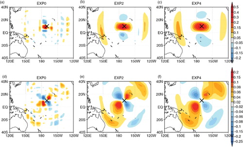
Figure 6 shows the analysis increments at initial time for the zonal and meridional wind fields in the single-observation experiments for EXP0, 2 and 4. Throughout the results, the location of the maximum wind increment does not exactly coincide with the observation location denoted by the black×, because there is a slight difference between the observation time and the initial time. The time correlations in the covariance, if any, do not influence the results and can be ignored. A localised horizontal structure of the increment is observed in EXP0 for both zonal and meridional winds, while a broader and smoother horizontal structure is shown along with increased spatial correlations (EXP2 in Fig. 6). The results of EXP3 through EXP5 are very similar for both zonal and meridional wind increments. That is, under the dominance of zonal flow in the basic state, the major zonal wind increment is located in the upstream region, which is west of the observation location. Also, to the southern (northern) part of that increment, the anti-cyclonic (cyclonic) circulation is deduced as seen in the meridional wind increment. The comparison of different spatial scales for the background error covariance model in eq. (9) shows that the covariance model reasonably spreads the information content by the spatial correlation obtained from EXP3 or larger spatial correlations. Note that there are no explicit correlations between state variables, and no balance constraints or damping of specific modes in the simple covariance matrix P ^b in eq. (8). Thus, cross correlations are introduced merely by the model dynamics (4D-aspect of the representer method). And, there seem to be two different regimes: continuity constraints close to the observation, and gravity waves further apart.

Fig. 6 Analysis increments for (a, b, c) zonal and (d, e, f) meridional wind fields in the single-observation experiments. EXP0 only uses variance information, while EXP2 and EXP4 used for a longer horizontal correlation. The observation location is denoted by the black ×. See Section 5.1 for more detail.

5.2. Identical twin experiments

The identical twin experiment is convenient methodology to test the usefulness of a given DA scheme, usually under a perfect model assumption. The true state is provided by a reference solution, which is a free simulation of the forecast model. The observations are sampled from this reference solution with proper measurement functions and the assumed measurement errors. By comparing with the true state, the performance of a given DA scheme can be easily evaluated.

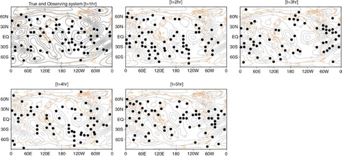
A set of identical twin experiments are designed to evaluate the developed variational DA system. The reference solution is obtained by integrating the SW standard test case 5 (isolated mountain) for 15 days, and the reference solution (nature run) is obtained by running NLM with an initial condition of the 14th day for a 6-hour assimilation window (Fig. 1c). For the observing system, the zonal winds located at the (2, 2) GLL point in each element are selected from the reference solution with probability 0.2, where random errors are added with the zero mean and variance of 1 m²s⁻².

The 334 observations are placed at the time of 1, 2, 3, 4 and 5-hour bins within a 6-hour assimilation window except at 0 and 6 hour bins for convenience. Figure 7 shows the ‘true’ zonal wind fields and randomly selected locations for observation. Note that observations are centred along the tropical zonal band due to the geometry of a cubed-sphere grid (Fig. 1a).

Fig. 7 Zonal wind fields (contours, ms⁻¹) for the true state at 1, 2, 3, 4 and 5 hours from the initial condition. Black dots indicate selected observational locations.

Background fields are chosen on the 13th day, which is one-day prior to the analysis time. The direct and indirect representer DA systems were tested with the zonal wind observations and the different covariance parameters shown in Section 3.4. The result from the direct representer system is given below, followed by a comparison with the results from the indirect representer system.

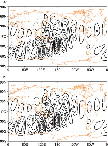
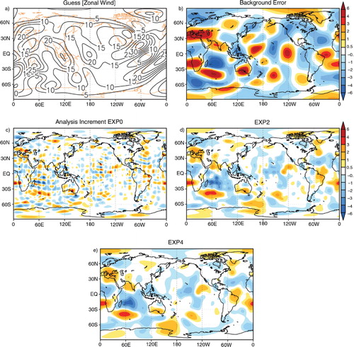
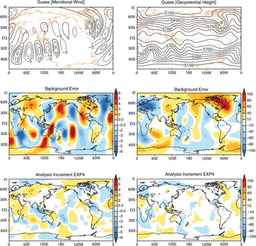
The representer matrix columns are computed by a representer function which requires TLM and ADM for each observation. After calculation of representer coefficients via the representer matrix, the analysis increment is obtained by the linear combination of the representer function. Figure 8 shows the zonal wind fields for background, background error field and the analysis increments for different covariance models. As shown in Fig. 8b, the maximum and minimum of the background errors are located over the eastern Indian Ocean. Analysis increments are shown for different covariance models. As in the single-observation experiments, the identical twin experiments with smaller length scales exhibit much localised increments (Fig. 8c), while smoother increments are shown for longer spatial length scales (Fig. 8d, e). For the analysis increment field, the locations at which background error is corrected are spatially similar to the locations of high-magnitude background errors, and the magnitude of the errors is reduced approximately by 30%.

Fig. 8 Zonal wind fields (ms⁻¹) for (a) guess and (b) the background error. The other panels (c–f) show the analysis increment for EXP0, EXP2 and EXP4. See Section 5.2 for more detail. Here, the background error is defined as true state minus background for direct comparison to the analysis increment (i.e., analysis minus background).

Although only the zonal wind component is assimilated in this study, the analysis increments for meridional wind and geopotential components also correct the background errors (Fig. 9). The errors in the meridional wind field are very similar to those in the zonal wind field, and the analysis increment has a similar spatial pattern to the background error field (left column in Fig. 9), but the magnitude of correction is about 12.6% less than the correction for the zonal wind. The analysis increment for the geopotential shows a similar pattern with 7.5% improvement compared to the background error (right column in Fig. 9). The improvement is still partially observed because the TLM and ADM spread out the observation information to other variables. Since the background error covariance P ^b shows only univariate correlation, multivariate correlations may be caused by the model dynamics. There are many ways in which the analysis increments need to be improved further partly because observations are rare around the polar-regions, and the covariance model is still univariate.

Fig. 9 Meridional wind (left column, ms⁻¹) and geopotential height (right column, gpm) fields for (a, b) initial guess, (c, d) background error and (e, f) analysis increment for EXP4. As in figure 8, the background error is defined as true state minus background.

The fact that the analysis increment does not fully compensate the initial first-guess error does not indicate that the analysis system is non-optimal. Indeed, the analysis is always some kind of mean of the background and the observations. So even if the observations correspond with the truth, the influence from the background will remain and any single analyses will deviate from the truth. Obviously, the larger background error length scales better correspond to the background error pattern. However, the outcome of a single forecast experiment cannot show the optimality or non-optimality of a given setup. That only can be achieved by statistical evaluation of a large number of forecast experiments. The system would be optimal if the actual statistical properties of the observations and of the background (here difference of sates 1 day apart) were properly described by the specified observational and background errors and covariances. Thus, this kind of identical twin experiment can only show that the analysis increments are reasonable: correct sign and reasonable cross correlations.

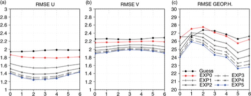
For the background and analysis fields, the forecast errors are calculated from the reference solution for the 6-hour assimilation window (Fig. 10). The analysis gives smaller forecast errors than the guess field for the wind components. The errors are also rather stable within the assimilation window. For the geopotential component, however, the forecast error from the EXP0 analysis is rather larger than that of the background fields. Also, the forecast error for the geopotential increases rapidly in the first 1-hour integration. This is partly due to the ignorance of balance properties between the state variables in the background error covariance (Section 3.4). While the EXP0 analysis is closer to the observation (see Table 1), the EXP5 experiment gives an analysis (and forecast) field closer to the true state (Fig. 10). This implies that the information spreading is very important and that the EXP0 analysis may be over-fitted to the observation.

Fig. 10 Root mean squared error of guess vs. analysis fields for (a) zonal, (b) meridional wind (ms⁻¹) and (c) geopotential height (gpm) fields within the assimilation window. The legends for lines are shown in (c).

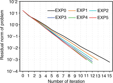
For the indirect representer system, a preconditioned conjugated gradient algorithm is adapted with a stopping criteria with (1) the maximum iteration of 30 or (2) reduction of the residual norm by 0.001% below the initial residual norm. For all cases, the iterations were terminated by the stopping criteria. Figure 11 shows the residual norm to the iterations indicating that about 15 integrations of TLM and ADM models are needed to obtain the analysis increment. The iterative optimisation is converged faster for longer horizontal length scales, and the number of iterations for convergence is given in the parentheses in Table 1. The minimisation problems in the experiments can be more efficiently solved with different stopping criteria. Note that, 334 integrations of the TLM and ADM are needed for direct representer. For the comparison of the analysis fields from direct and indirect representer systems, the two fields are indistinguishable from each other, and their difference is O(10⁻⁵), and the other fields are also similar (figure not shown).

Fig. 11 Residual norm vs. the iteration number for optimisation.

The similarity of both methods can be confirmed by comparing the observational part of the cost function for analysis (or misfit of analysis fields at the 334 observations) in a series of twin experiments (Table 1). The misfit of background fields at the observation locations is initially Jo_init=1996.2858000307174. Both direct and indirect methods show the similar results for the misfits of analysis fields at the observation locations that are much reduced. That is, the misfits of analysis fields are only 0.85% for EXP0 that is the smallest correlation length scale, and 19% for EXP5 that is the largest correlation length scale, possibly because the smoothing procedure in the covariance model influences the analysis values at the locations by neighbourhood values. In Table 1, the representer coefficient β (1) of the representer function for the 1st observation is compared for the direct and indirect representer systems. At least four digits are identical for the coefficient β (1).

Table 1. Final observational cost function J_o and coefficient of the representer function for the 1st observation. The initial value for the observational cost function is Jo_initial=1996.2858000307174. The number of each iteration for convergence in the indirect method is parenthesised

Jo_final	β(1)
EXP0	Dir.	16.887891232005309	−7.97446808307937238E-002
Indir. (15)	16.887880548841444	−7.97402736327472439E-002
EXP1	Dir.	74.140407110010187	−2.1577598478099236E-001
Indir. (13)	74.140422305656671	−2.1577268687457979E-001
EXP2	Dir.	152.96505052357273	−3.4533675376322964E-001
Indir. (12)	152.96504225347354	−3.4532035046868231E-001
EXP3	Dir.	232.55411655531199	−4.4839433805313200E-001
Indir. (12)	232.55410737568016	−4.4836725194073235E-001
EXP4	Dir.	305.25529998879114	−5.2857625785335349E-001
Indir. (12)	305.25529336002552	−5.2855427089217744E-001
EXP5	Dir.	371.32774817521414	−5.8911482799744241E-001
Indir. (11)	371.32773491110731	−5.8910244555192393E-001

6. Summary

In this study, direct and indirect representer-based variational DA systems were developed for the spectral element SW system, which include development and verification of TLM and ADM for the forecast model, a simple background error covariance model, and main representer algorithms. The characteristics of the covariance model were evaluated with different horizontal length scales by the suite of single-observation experiments. The developed direct and indirect representer algorithms were evaluated and compared in a series of identical twin experiments. In both methods, the analysis increments were obtained by the weighted linear combination of representer functions. The weights, called the representer coefficients for the representer functions, were calculated explicitly in the direct method and iteratively in the indirect method. However, this study does not cover various components of variational DA systems, such as outer loop configuration to account for non-linearity, linearisation of simplified physics, and more advanced covariance modelling that need for the further development.

The components of the direct and indirect representer methods were validated in various DA tests and the developed representer-based variational DA system yielded satisfactory results for the spectral element SW model. The indirect representer method seems to be practical enough to be run near-real time with less than 15 iterations of the minimisation algorithms to get more accurate initial conditions. This study can be further extended for improvement of geostrophic balance relationships in the covariance model, covariance parameter estimation, efficient and reliable stopping criteria for optimisation, more realistic simulations of the observing system and so on. The development and verification for the SW system presented here have important practical applications for further development of tangent linear and ADMs for three-dimensional primitive hydrostatic models based on the spectral element methods such as the HOMME, which is currently being developed (Kim et al., 2014). The forward and ADMs for the spectral element models can be employed in various inverse problems including traditional DA, parameter estimation, and model sensitivity and stability analysis. The developed TLM and ADM will be evaluated in a three-dimensional configuration, and the efforts will lead to the development of a future DA system for spectral models like HOMME and the KIAPS model.

7. Acknowledgements

The authors would like to thank the anonymous reviewers for many valuable comments and suggestions, which greatly improved the presentation of this paper. This work has been carried out through the R&D project on the development of global numerical weather prediction systems of Korea Institute of Atmospheric Prediction Systems (KIAPS) funded by Korea Meteorological Administration (KMA).

References

- Bannister R. N . A review of forecast error covariance statistics in atmospheric variational data assimilation. I: characteristics and measurements of forecast error covariances. Q. J. Roy. Meteorol. Soc. 2008a; 134: 1951–1970.
- Bannister R. N . A review of forecast error covariance statistics in atmospheric variational data assimilation. II: modeling the forecast error covariance statistics. Q. J. Roy. Meteorol. Soc. 2008b; 134: 1971–1996.
- Bennett A. F . Inverse methods in physical oceanography, monographs on mechanics and applied mathematics. 1992; Cambridge University Press, Cambridge.
- Bennett A. F . Inverse modeling of the ocean and atmosphere. 2002; New York: Cambridge University Press. 225 pp.
- Bennett A. F. , McIntosh P. C . Open ocean modeling as an inverse problem: tidal theory. J. Phys. Oceanogr. 1982; 12: 1004–1018.
- Bennett A. F. , Thorburn M. A . The generalized inverse of a nonlinear quasigeostrophic ocean circulation model. J. Phys. Oceanogr. 1992; 22: 213–230.
- Bouttier F. , Courtier P . Data assimilation concepts and methods, ECMWF meteorological training lecture notes. 1999; ECMWF. 1–58.
- Chua B. S. , Bennett A. F . An inverse ocean modeling system. Ocean. Model. 2001; 3: 137–165.
- Chua B. S. , Zaron E. , Xu L. , Baker N. , Rosmond T . Park S. K. , Xu L . Recent applications in representer-based variational data assimilation. Data Assimilation in Atmospheric, Oceanic and Hydrologic Application. 2013; Berlin: Springer-Verlag. 287–301.
- Courtier P . Dual formulation of four-dimensional data assimilation. Quart. J. Royal. Meteo. Soc. 1997; 123: 2449–2461.
- Courtier P. , Talagrand O . Variational assimilation of meteorological observations with the direct and adjoint shallow-water equations. Tellus A. 1990; 42: 531–549.
- Daley R . Atmospheric data analysis. 1991; New York: Cambridge University Press.
- Dennis J. , Fournier A. , Spotz W. F. , St-Cyr A. , Taylor M. A. , co-authors . High resolution mesh convergence properties and parallel efficiency of a spectral element atmospheric dynamical core. High Perf. Comp. Appl. 2005; 19: 225–235.
- Dennis J. M. , Edwards J. , Evans K. J. , Guba O. , Lauritzen P. H. , co-authors . CAM-SE: A scalable spectral element dynamical core for the Community Atmosphere Model. High Perf. Comp. Appl. 2012; 26: 74–89.
- Derber J. , Rosati A . A global oceanic data assimilation system. J. Phys. Oceanogr. 1989; 19: 1333–1347.
- Fisher M. , Andersson E . Developments in 4d-Var and Kalman filtering. 2001. ECMWF Tech. Memo. 347 (available from ECMWF, Shinfield Park, Reading, Berkshire, RG2 9AX, UK).
- Giering R. , Kaminski T . Recipes for adjoint code construction. ACM Trans. Math. Software. 1997; 24: 437–474.
- Hollingsworth A. , Lonnberg P . The statistical structure of short range forecast errors as determined from radiosonde data. Part I: the wind field. Tellus A. 1986; 38: 111–136.
- Holm E. V . Lecture note on assimilation algorithms. 2008; ECMWF. 30p.
- Kim S. , Jung B.-J. , Jo Y . Development of a tangent linear model (version 1.0) for the High-Order Method Modelling Environment dynamical core. Geosci. Model Dev. 2014; 7: 1175–1196.
- Kurapov A. L. , Egbert G. D. , Allen J. S. , Miller R. N . Representer-based variational data assimilation in a nonlinear model of nearshore circulation. J. Geo. Res. C11019 . 2007; 1–18.
- Kurapov A. L. , Egbert G. D. , Allen J. S. , Miller R. N . Representer-based analyses in the coastal upwelling system. Dynam. Atmos. Oceans. 2009; 48: 198–218.
- Lawless A. S. , Nichols N. K. , Ballard S. P . A comparison of two methods for developing the linearization of a shallow-water model. Q. J. R. Meteorol. Soc. 2003; 129: 1237–1254.
- Mandel J . Efficient implementation of the ensemble Kalman filter. 2006. CCM Report 231, University of Colorado Denver.
- Moore A. M . Schiller A , Grassington G. B . Adjoint data assimilation methods. Operational Oceanography in the 21st Century. 2011; Springer. 351–380.
- Moore A. M. , Hernan G. A. , Lorenzo E. D. , Cornuelle B. D. , Miller A. J. , co-authors . A comprehensive ocean prediction and analysis system based on the tangent linear and adjoint of a regional ocean model. Ocean Model. 2004; 7: 227–258.
- Nair R. D. , Thomas S. J. , Loft R. D . A discontinuous galerkin global shallow water model. Mon. Wea. Rev. 2005; 133: 876–888.
- Ngodock H. E. , Smith S. R. , Jacobs G. A . Cycling the representer algorithm for variational data assimilation with the Lorenz Attractor. Mon. Wea. Rev. 2007; 135: 373–386.
- Ngodock H. E. , Smith S. R. , Jacobs G. A . Park S. K. , Xu L . Cycling the Representer Method with Nonlinear Models. Data Assimilation for Atmospheric, Oceanic and Hydrologic Applications. 2009; Berlin: Springer-Verlag. 321–340.
- Parrish D. F , Derber J. C . The National Meteorological Center's spectral statistical interpolation analysis system. Mon. Wea. Rev. 1992; 120: 1747–1763.
- Rabier F . Overview of global data assimilation developments in numerical weather prediction centres. Q. J. Roy. Meteorol. Soc. 2005; 131: 3215–3233.
- Rabier F. , Järvinen H. , Klinker E. , Mahfouf J.-F. , Simmons A . The ECMWF implementation of four-dimensional variational assimilation. I: experimental results with simplified physics. Q. J. Roy. Meteorol. Soc. 2000; 126: 1143–1170.
- Ronchi C. , Iacono R. , Paolucci P. S . The “cubed sphere”: a new method for the solution of partial differential equations in spherical geometry. J. Comput. Phys. 1996; 124: 93–114.
- Rosmond T. , Xu L . Development of NAVDAS-AR: nonlinear formulation and outer loop tests. Tellus A. 2006; 58A: 45–58.
- Sadourny R . Conservative finite-difference approximations of the primitive equations on quasi-uniform spherical grids. Mon. Wea. Rev. 1972; 100: 136–144.
- Smith S. R. , Ngodock H. E . Cycling the representer method for 4D-variational data assimilation with the Navy Coastal Ocean Model. Ocean Model. 2008; 24: 92–107.
- Taylor M. , Tribbia J. , Iskandrani M . The spectral element method for the shallow water equations on the sphere. J. Comput. Phys. 1997; 130: 92–108.
- Weaver A. , Courtier P . Correlation modelling on the sphere using a generalized diffusion equation. Q. J. R. Meteo. Soc. 2001; 127: 1815–1846.
- Williamson D. L. , Drake J. B. , Hack J. J. , Jakob R. , Swarztrauber P. N . A standard test set for numerical approximations to the shallow water equations in spherical geometry. J. Comput. Phys. 1992; 102: 211–224.
- Xu L. , Daley R . Towards a true 4-dimensional data assimilation algorithm: application of a cycling representer algorithm to a simple transport problem. Tellus A. 2000; 52: 109–128.
- Xu L. , Daley R . Data assimilation with a barotropically unstable shallow water system using representer algorithms. Tellus. 2002; 54: 125–137.
- Xu L. , Rosmond T. , Daley R . Development of NAVDAS-AR. Formulation and initial tests of the linear problem. Tellus. 2005; 57: 546–559.
- Zhu K. , Navon I. M. , Zou X . Variational data assimilation with a variable resolution finite-element shallow-water equation model. Mon. Wea. Rev. 1994; 122: 946–965.
- Zou X. , Vandenberghe F. , Pondeca M. , Kuo Y.-H . Introduction to adjoint techniques and the MM5 adjoint modeling system. 1997. NCAR Tech. Note NCAR/TN-435-STR.