Roles of an upper-level cold vortex and low-level baroclinicity in the development of polar lows over the Sea of Japan

Abstract

The relationship between a synoptic-scale, upper-level cold vortex and a meso-α scale polar low (PL) over the Sea of Japan, and the role played by low-level baroclinicity in the development of the PL were investigated. We examined three PLs from the perspective of potential vorticity (PV) and energy budgets, using mesoscale analysis data with a horizontal resolution of ~11 km. During the development stage of each PLs, a meso-α scale upper-level PV (UPV) anomaly, which intrudes to around the 700–600 hPa level and which is just a part of a synoptic-scale PV anomaly accompanying the cold vortex, moved to the west side of a low-level PL. The PL was located in a wide region of low static stability in the lower troposphere. These conditions suggested that the synoptic-scale cold vortex, accompanied by a cold dome and the different scales of UPV anomalies, played a role in creating a favourable environment for the PL development. One of the common characteristics of the PL cases studied here was that, in contrast to the low-level PL, the upper-level disturbance associated with the meso-α scale UPV anomaly showed no development at all. This is likely because of the mobile UPV anomaly cut off from its source. Low-level baroclinicity, which varied with time, was an important factor in differentiating the PL shape and the energy sources necessary for PL development. Furthermore, the strength of baroclinicity, through its enhancement of mesoscale fronts and convection, affected diabatic processes, as well as baroclinic development.

• mesoscale front
• PV anomaly
• energy budget analysis

1. Introduction

Polar lows (PLs) generally develop over the ocean, and they decay very rapidly after landfall. Their horizontal scale is less than 1000 km, much smaller than that of extratropical cyclones. PLs cause heavy snowfall and wind gusts in a small area, which can have serious impacts on socioeconomic activities. Over the Sea of Japan, PLs are frequently observed during winter, and wind gusts from these PLs have caused accidents in Japan, including a train blown off a railway bridge. To mitigate disasters due to PLs, the characteristics of PLs over the Sea of Japan have been actively studied since the 1980s by using in situ observations and satellite observations (e.g. Asai and Miura, 1981; Asai, 1988; Ninomiya and Hoshino, 1990; Yamagishi et al., 1992).

Many studies have investigated the structure and mechanism of development of PLs. Shapiro et al. (1987) carried out the aircraft measurements within a PL over the Norwegian Sea and revealed the existence of a mesoscale frontal structure. Hewson et al. (2000) reported that the mesoscale frontal structure of PLs over the North Atlantic Ocean corresponded closely to the frontal structure of the Shapiro and Keyser model (1990) for explosively developing extratropical cyclones. Typically, PLs are characterised by comma and spiraliform cloud patterns.

In numerous case studies and numerical experiments, various mechanisms have been proposed for the development of PLs, including baroclinic instability (e.g. Mansfield, 1974; Duncan, 1977; Reed and Duncan, 1987; Tsuboki and Wakahama, 1992), the conditional instability of the second kind (CISK) (e.g. Rasmussen, 1979; Craig and Cho, 1988), the wind-induced surface heat exchange (WISHE) (e.g. Emanuel and Rotunno, 1989; Craig and Gray, 1996), and a combination of moist baroclinity and CISK (e.g. Sardie and Warner, 1983). With respect to baroclinicity, reverse-shear conditions, wherein the thermal wind is antiparallel to the flow, are favourable for PL development (e.g. Kolstad, 2006). In addition, some studies have suggested that an upper-level potential vorticity (UPV) (e.g. Montgomery and Farrell, 1992; Mailhot et al., 1996) and physical processes such as condensational heating and turbulent heat fluxes from the sea surface play important roles in PL development (e.g. Bresch et al., 1997; Yanase et al., 2004; Føre et al., 2012; Føre and Nordeng, 2012). Taken together, the findings of these studies indicate that the development mechanism of PLs differs from case to case, depending on environmental conditions. Thus, how and in what environments PLs develop are not well understood at present.

Yanase and Niino (2007) used a high-resolution non-hydrostatic model under idealised atmospheric conditions to model the relationship between environmental baroclinicity and PL characteristics, and their results provide a basis for exploring the mechanism of PL development. They found that PLs that develop in weakly baroclinic environments are characterised by a small, quasi-axisymmetric vortex, whereas PLs that develop in strongly baroclinic environments characteristically have a comma-shaped cloud pattern. Their energy budget analysis revealed that strong baroclinicity enabled PLs to develop faster and to become stronger than weak baroclinicity did.

One important factor in PL development is the presence of UPV anomalies. Montgomery and Farrell (1992) proposed a two-stage conceptual model based on a non-linear geostrophic momentum model. The first stage is a spin-up of a low-level incipient vortex induced by UPV anomalies. During the second stage, low-level potential vorticity (PV) anomalies generated by diabatic heating help maintain the intensity of the vortex. This effect of UPV on low-level vortex development has been confirmed by case studies (Grønås and Kvamstø, 1995; Mailhot et al., 1996; Rasmussen et al., 1996; Claud et al., 2004; Bracegirdle and Gray, 2009).

In the Sea of Japan, PLs are usually accompanied by a comma-shaped cloud pattern (Yarnal and Henderson, 1989), and they have a warm core structure in the lower troposphere (Asai and Miura, 1981; Ninomiya and Hoshino, 1990). An upper-level cold vortex is often one of the synoptic characteristics associated with a PL (e.g. Ninomiya et al., 1990; Lee et al., 1998; Fu et al., 2004; Wu et al., 2011). Tsuboki and Wakahama (1992), who used radiosonde observations to investigate the mechanism of PL development over the Sea of Japan as a linear instability problem of baroclinic flow, indicated that the observed PLs were characterised by two unstable modes with wavelengths of 200–300 km and 500–700 km. Yanase et al. (2004) performed numerical experiments that showed that condensational heating was important in the development of a PL under sufficiently moist atmospheric conditions and low static stability. In addition, turbulent heat fluxes from the sea surface help maintain long-term low static stability, although they strongly, but indirectly, influence the PL development.

Numerous studies on PLs over the Sea of Japan have shown that they develop under low-level baroclinicity in connection with the approach of a synoptic-scale upper-level cold vortex. However, the relationship between the synoptic-scale upper-level cold vortex and a meso-α scale PL, and the roles of low-level baroclinicity in the development of the PL are still not well understood. On the basis of a piecewise PV inversion diagnosis, Wu et al. (2011) showed that a UPV anomaly associated with a cold vortex could induce a synoptic-scale cyclonic circulation in the lower troposphere, and could contribute to deepening of a surface PL. The induction of a meso-α scale PL, however, must involve some sort of mesoscale processes under the influence of such a synoptic-scale cold vortex. To clarify these processes, mesoscale PV distributions during the development of PLs must be analysed in detail. In addition, how low-level baroclinicity contributes to the differentiation of the PL characteristics, such as its shape, frontal activity and development processes, needs to be determined through case studies.

Recently, objective analysis data with fine resolution (approximately 10 km) have become available. In these data, the analysed fields are expected to be closer to the actual atmospheric field than fields simulated by a numerical model. Such data enable structures such as fronts and mesoscale PV distributions to be examined, and energy budgets of real PLs to be explored.

In this study we analysed three PLs (Fig. 1a) that occurred over the Sea of Japan to clarify the roles of the upper-level cold vortex and low-level baroclinicity in the development of PLs, in particular, from the perspective of PV and the energy budget. We used mesoscale analysis data of the Japan Meteorological Agency (JMA) with a horizontal resolution of approximately 11 km for this analysis. In addition, we investigated whether the PLs have a mesoscale frontal structure, and the baroclinic interaction between each low-level PL and the upper-level disturbance. Although baroclinic instability in PLs was previously examined as a linear instability problem (e.g. Mansfield, 1974; Duncan, 1977; Reed and Duncan, 1987; Tsuboki and Wakahama, 1992), the three-dimensional baroclinic structure associated with PLs in the real atmosphere is not well investigated. First, we show the results of our frontal analysis. Then we carry out a mesoscale PV analysis to examine what processes caused each meso-α scale PL to develop under the existence of the synoptic-scale cold vortex, while taking account of baroclinic interaction. We also examine the role of low-level baroclinicity by conducting potential and kinetic energy budget analyses.

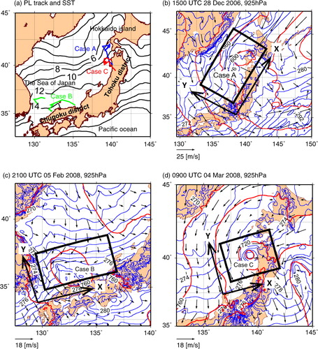
Fig. 1 (a) Sea surface temperatures (SSTs) (solid contours, every 2°C) averaged from December to March for the years 2003–2012, and the tracks of the examined PLs: case A (blue line), case B (green lines) and case C (red line). The X–Y coordinate system, geopotential height (red contours), potential temperature (blue contours) and horizontal wind (vectors) of each PL in the middle of its lifetime: (b) case A (geopotential height, every 60 m; potential temperature, every 2 K); (c) case B (geopotential height, every 20 m; potential temperature, every 1 K); (d) case C (geopotential height, every 20 m; potential temperature, every 1 K).

We explain the data and methods used for the PV and energy budget analyses in section 2, and we describe each investigated PL case in section 3. In section 4, we present the results of our frontal, PV and energy budget analyses, and in section 5, we discuss the processes influenced by UPV, the baroclinic interaction and favourable conditions for PL development. Finally, in section 6 we present our conclusions.

2. Data and methodology

2.1. Data

We used 3-hourly operational mesoscale analysis data calculated by the JMA four-dimensional variational data assimilation (4D-Var) system. The 4D-Var system is based on the JMA Meso-Scale Model (MSM), which is an updated version of the JMA non-hydrostatic mesoscale model (Saito et al., 2006). The horizontal resolution of the dataset is 0.125° in longitude and 0.1° in latitude (approximately 11 km). The number of vertical layers is 16 (1000, 975, 950, 925, 900, 850, 800, 700, 600, 500, 400, 300, 250, 200, 150 and 100 hPa). Satellite, radar, wind profiler and in situ observations were assimilated. Note that the 3-hourly analysis data do not guarantee dynamic consistency. Moreover, the values of vertical winds over mountain areas are unrealistic and excessively high before April 2007, because the Z* coordinate, used as the vertical coordinate of the MSM, follows the topography. For this reason, in the energy budget analysis we arbitrarily excluded parts of the domain where vertical velocities were unrealistic and excessively high. This exclusion is not a serious problem in this study because the energy budget analysis was conducted mostly over the sea, where the three PLs mainly occurred. We used synoptic weather charts provided by the JMA (surface and 500 hPa), radar composite imagery observed by JMA operational radar network and infrared geostationary satellite imagery from the Multi-functional Transport Satellite (MTSAT-1R) 10.8 µm IR channel to investigate synoptic and meso-α scale features associated with the three PLs. We also used Merged satellite and in situ data Global Daily Sea Surface Temperatures (MGDSSTs) (Kurihara et al., 2006) to show sea surface temperatures (SSTs) over the Sea of Japan.

2.2. Definitions

We used the formulation of Emanuel et al. (1987) to calculate diabatic heating:1 where θ is potential temperature, θ _e is equivalent potential temperature, p is pressure, t is time, ω is the vertical p-velocity (=dp/dt), Γ _m is the moist adiabatic lapse rate and Γ _d is the dry adiabatic lapse rate.

We used Ertel's PV on isobaric and isentropic surfaces. For simplicity, an air parcel of which the PV differs from the surrounding PV values is termed a ‘PV anomaly’. In our analysis of the PV distribution, we introduce the Rossby height H _R (Van Delden et al., 2003), which is used as a qualitative indication of the vertical penetration of the induced flow structure below the location of a UPV anomaly (Hoskins et al., 1985).2 where L is the horizontal scale of a PV anomaly, f is the Coriolis parameter, ζ _θ is the relative vorticity on an isentropic surface averaged over the scale L and N is the Brunt-Väisälä frequency in the environment, which is calculated by3 where g is gravitational acceleration. The bracket ([]) indicates the vertical average from 925 to 600 hPa. For simplicity, we approximate f as ~10⁻⁴ s ⁻¹ (around 40°N) in this study.

2.3. Energy budget formulation

We performed an energy budget analysis using a specified X–Y coordinate system for each PL (Fig. 1b–d) to clarify the role of low-level baroclinicity in terms of the dynamics and thermodynamics of PL development. The area covered by the coordinate system associated with each PL was determined as follows: The values of potential temperature at a zonal boundary (parallel to the Y axis) are mainly the same as those at the opposite boundary in the middle of the lifetime of each PL (Fig. 1b–d). Therefore, representative winds and potential temperatures could be expressed as basic fields in each X–Y coordinate system. The zonal distance was determined as the distance of about one wavelength expressed in terms of the deviations from the zonally averaged potential temperature in the middle of the lifetime of each PL. The distance in the Y direction was chosen to be within the disturbance associated with the targeted PL, excluding areas of unrealistic and excessively high vertical wind.

The potential and kinetic energy budget analyses are based on formulations derived from hydrostatic primitive equations because hydrostatic model was used in a part of the 4D-Var system before April 2007. In the following formulations, the zonal average is indicated by an overbar and the deviation from the zonal average is indicated by adding a prime to the variable. Eddy potential energy (EPE, Pe) is defined as4 and eddy kinetic energy (EKE, Ke) is defined as5 where6 θ ₀ is the reference potential temperature (which is a function of p), and u and v are the zonal (X) and meridional (Y) velocity components, respectively.

The EPE budget equation is7 where Pe* is defined as θ^′2/2, α′ is the deviation from the zonally averaged specific volume, π is the Exner function (=(p/p ₀) ^κ , κ=R/c _p ), R is the specific gas constant for dry air, c _p is the specific heat at constant pressure and p ₀ is 1000 hPa. The first to sixth terms on the right-hand side (rhs) of eq. (7) indicate the advection of EPE due to the zonal mean wind () and eddies (PeAdv’), the seventh term is the conversion from mean potential energy (MPE) to EPE ([Pm, Pe]), which we hereafter call ‘baroclinic development’, the eighth and ninth terms are the conversion from EPE to EKE ([Pe, Ke]) and the generation of EPE by diabatic heating Q ([Q, Pe]), respectively; hereafter, the last is called ‘diabatic development’. The tenth term is the subgrid-scale dissipation (Diss), which is evaluated as the difference between , calculated using a centred difference, and the sum from the first term to the ninth term, in this study. Then, we multiply EPE and all of the terms in eq. (7) by , so that EPE and EKE have the same dimensions.

The equation of the EKE budget is8 where Ke* is defined as , and Φ (=gz) is the geopotential. The first to sixth terms on the rhs of eq. (8) indicate the advection of EKE by zonal mean winds () and eddies (KeAdv’), the seventh and eighth terms are the conversion from mean kinetic energy (MKE) to EKE ([Km, Ke]), the ninth and tenth terms are the conversion from MKE to EKE by convection and vertical shear of the basic zonal wind (Vert), the eleventh term is the conversion from EPE to EKE ([Pe, Ke]) and the twelfth to fourteenth terms represent the convergence of geopotential energy fluxes by disturbances (GEF). The fifteenth term (Diss) is evaluated as the same way as that in the EPE budget.

We examined how energy sources, such as [Pm, Pe] (baroclinic development) and [Q, Pe] (diabatic development), necessary for PL development differed among the three studied PLs.

3. Three PL cases

We investigated the development of three PLs over the Sea of Japan (Fig. 1a). The first PL (case A) occurred off the western coast of Hokkaido Island from 0000 UTC on 28 December to 0300 UTC on 29 December 2006. The second PL (case B) occurred off the north coast of Chugoku district from 0600 UTC on 5 February to 1200 UTC on 6 February 2008. The third PL (case C) occurred off the western coast of Tohoku district from 0600 UTC on 3 March to 1200 UTC on 5 March 2008. All three PLs were identified by using satellite imagery and radar observations and were well reproduced by the analysis data. In addition, each could be analysed within its X–Y coordinate system from the time of its initiation to maturity.

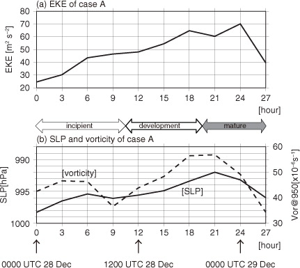
In case A, the PL developed in a cold air outbreak on the western flank of a synoptic-scale extratropical cyclone over the sea off the eastern coast of Hokkaido Island (Fig. 2a). From 0000 UTC to 0900 UTC on 28 December, low-level cold advection was stronger in the western part of the Sea of Japan than in its eastern part (not shown). As a result, there was a strong zonal temperature gradient in the low-level atmosphere (not shown). Convection gradually became enhanced off western Hokkaido Island (Fig. 3a), and at 500 hPa, a synoptic-scale cold vortex approached the area of convection (not shown). After 1200 UTC on 28 December, convective clouds started to roll up cyclonically, causing a comma-shaped cloud pattern to form (Fig. 3b). The PL reached maturity by 2100 UTC on 28 December, and the 500 hPa cold-core vortex passed over the PL at around 0000 UTC on 29 December (Fig. 2b). After 0000 UTC on 29 December, the PL made landfall in Tohoku district and then disappeared rapidly. At the end of its lifetime, the PL acquired a spiraliform cloud pattern (Fig. 3c and 3d). The evolution of the mean EKE averaged from 925 to 800 hPa and over the X–Y domain (Fig. 1b), the sea level pressure (SLP) at the PL centre, and the relative vorticity at 950 hPa averaged over the X–Y domain (Fig. 4) all indicated that the PL developed primarily from 1200 UTC to 1800 UTC on 28 December. We defined this period as the development stage of the case A PL. In addition, we defined the period before (after) the development stage as the incipient (mature) stage of case A.

Fig. 2 Weather charts provided by the JMA: (a) Surface and (b) 500 hPa weather charts at 0000 UTC on 29 December 2006, (c) surface and (d) 500 hPa weather charts at 0000 UTC on 6 February 2008, and (e) surface and (f) 500 hPa weather charts at 0000 UTC on 5 March 2008.

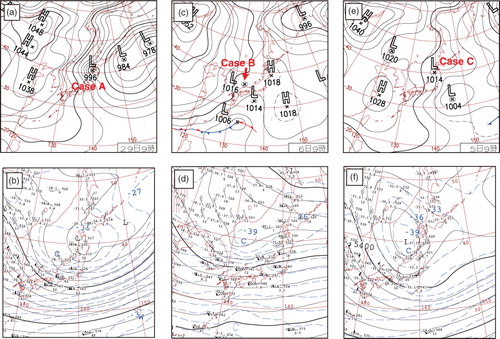
Fig. 3 Case A. Satellite images: (a) 0600 UTC on 28 December (incipient stage), (b) 1800 UTC on 28 December (development stage) and (c) 0300 UTC on 29 December 2006 (mature stage). (d) Radar composite image at 0300 UTC on 29 December 2006 (mature stage).

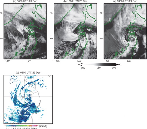
Fig. 4 Case A. Time evolution of parameters from 0000 UTC on 28 December to 0300 UTC on 29 December 2006: (a) EKE, averaged horizontally over the X–Y domain (see Fig. 1b) and vertically from 925 to 800 hPa. (b) Sea level pressure (SLP) at the PL centre (solid line), and relative vorticity, averaged horizontally over the X–Y domain at 950 hPa (dashed line).

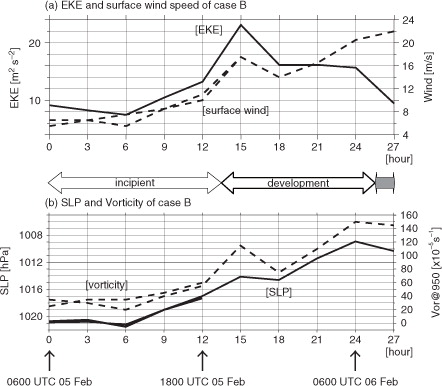
In case B, the PL developed over the western part of the Sea of Japan, more than 1000 km north of the location of a developing extratropical cyclone (Fig. 2c). Two pre-disturbances appeared over the area between 0600 UTC and 1800 UTC on 5 February 2008 (shown as two tracks in Fig. 1a). By 2100 UTC on 5 February, the southern pre-disturbance had developed into a PL with a comma-shaped cloud pattern off the north coast of Chugoku district (Fig. 5a and 5b), and the northern pre-disturbance had gradually dissipated. Then, from 0000 UTC to 0600 UTC on 6 February 2008, it developed further (Fig. 5c and 5d). During this period, a short upper-level trough passed through the PL area (Fig. 2d). The evolution of the mean EKE averaged from 925 hPa to 800 hPa and over the X–Y domain (Figs. 1c and 6a) did not show a maximum at around 0600 UTC on 6 February, mainly because the scale of the PL had gradually decreased. However, the evolution of maximum surface wind speed, SLP at the PL centre, and maximum relative vorticity at 950 hPa (Fig. 6) indicated that the PL had reached maturity by 0600 UTC on 6 February. Subsequently, the PL made landfall and rapidly disappeared. The upper-level cold vortex in case B, unlike that in case A, was located 400 km north of the PL (Fig. 2d). We defined the period when the PL was approaching maturity from 2100 UTC on 5 February to 0600 UTC 6 February as the development stage of case B. In addition, we defined the period before (after) the development stage as the incipient (mature) stage of case B.

Fig. 5 Case B. Satellite images: (a) 1500 UTC on 5 February (incipient stage), (b) 2100 UTC on 5 February (development stage) and (c) 0300 UTC on 6 February 2008 (development stage). (d) Radar composite image at 0300 UTC on 3 February 2008 (development stage).

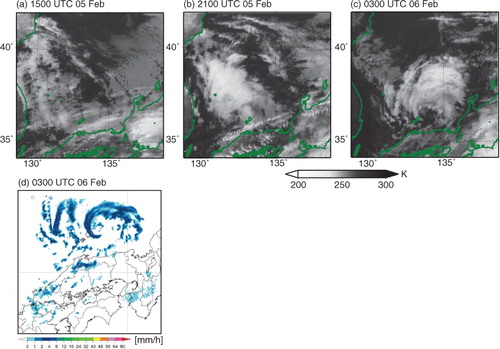
Fig. 6 Case B. Time evolution of parameters from 0600 UTC on 5 February to 0900 UTC on 6 February 2008: (a) EKE, averaged horizontally over the X–Y domain and vertically from 925 to 800 hPa (solid lines), and maximum surface wind (dashed lines). (b) SLP at the PL centre (solid lines) and maximum relative vorticity at 950 hPa (dashed lines; one for each incipient disturbance). Values at 1200 UTC on 6 February 2008 are excluded because half of the PL was outside of the X–Y domain.

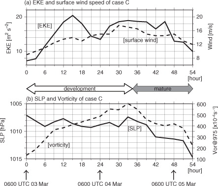
In case C, the PL developed on the north-western flank of an extratropical cyclone (Fig. 2e). Satellite imagery showed that convective clouds appeared in the northwest quadrant, but no clouds were apparent on the south side or in the centre of the PL during the first half of the PL's lifetime (from 0600 UTC on 3 March to 1500 UTC on 4 March 2008, Fig. 7a and 7b). Then, during the second half of its lifetime (from 1800 UTC on 4 March to 1200 UTC on 5 March 2008, Fig. 7c and 7d), it acquired a spiraliform cloud pattern accompanied by convection, which rolled up cyclonically. At 0600 UTC on 5 March, the PL made landfall over Tohoku district and then disappeared. The PL remained quasi-stagnant for about two days after it occurred. Initially, a synoptic-scale cold vortex was located about 800 km northwest of the PL at 500 hPa (not shown). This vortex moved southward while weakening, and it passed over the PL at around 0600 UTC on 5 March (Fig. 2f). The evolution of the mean EKE averaged from 925 to 800 hPa and over the X–Y domain (Fig. 1d), maximum surface wind speed, SLP at the PL centre and relative vorticity at 975 hPa averaged over the area within a radius of 35 km from the centre (Fig. 8) showed two local intensity maxima, at 2100 UTC on 3 March and at 1500 UTC on 4 March. We defined the period from 0600 UTC on 3 March to 1500 UTC on 4 March 2008 as the development stage of case C, and the period after the development stage as the mature stage of case C. This PL was weaker than the case A PL and of almost the same intensity as the case B PL (Figs. 4a, 6a and 8a).

Fig. 7 Case C. Satellite images: (a) 2100 UTC on 3 March (development stage), (b) 1200 UTC on 4 March (development stage) and (c) 0300 UTC on 5 March 2008 (mature stage). (d) Radar composite image at 0300 UTC on 5 March 2008 (mature stage).

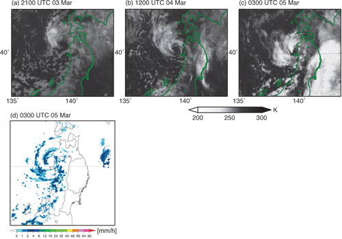
Fig. 8 Case C. Time evolution of parameters from 0600 UTC on 3 March to 1200 UTC on 5 March 2008: (a) EKE, averaged horizontally over the X–Y domain and vertically from 925 to 800 hPa (solid line), and maximum surface wind (dashed line). (b) SLP at the PL centre (solid line), and relative vorticity averaged within a 35 km radius of the centre at 975 hPa (dashed line).

4. Results

We investigated the roles of upper-level cold vortices and low-level baroclinicity in the development of the three PLs from the perspective of PV and energy budgets. First, however, we examined whether the PLs had a mesoscale frontal structure such as that seen in PLs over the Norwegian Sea (e.g. Shapiro et al., 1987; Hewson et al., 2000).

4.1. Frontal analysis

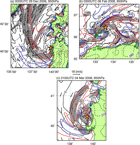
Following Shapiro et al. (1987), we refer to a mesoscale baroclinic zone as a front in this study. Figure 9 shows horizontal distributions of potential temperature, vertical wind and horizontal gradients of potential temperature exceeding 3 K per 100 km at 950 hPa of case A at the mature stage, of case B at the development stage and of case C at the mature stage. All three PLs had a low-level warm core surrounded by a sharp horizontal potential temperature gradient. Moreover, air motion was strongly upward (downward) on the warmer (colder) side of the potential temperature gradient. This gradient was strengthened by the confluence of horizontal winds or horizontal wind shear, or both, at the lower part of the front (~950 hPa), and by diabatic heating at the upper part of the front (~850 hPa) in all three PLs (not shown). Thus, all three PLs had a distinct mesoscale frontal structure, which was accompanied by active convection. The frontal structure did not depend on whether the PL had a comma-shaped or a spiraliform cloud pattern.

Fig. 9 Map views of potential temperature (dashed contours; every 1 K), upward wind (red contours, drawn at 20, 80 and 160 hPa h⁻¹) and downward wind (blue contours, drawn at 20, 80 and 160 hPa h⁻¹) at 950 hPa. (a) Case A at 0000 UTC on 29 December 2006 (mature stage); (b) case B at 0300 UTC on 6 February 2008 (development stage); and (c) case C at 2100 UTC on 4 March 2008 (mature stage). Shading indicates a horizontal gradient of potential temperature greater than 3 K per 100 km. W, warm core; vectors, horizontal wind; and orange star, PL centre. Vertical winds over land are masked out because of unrealistic and excessively high values (see subsection 2.1).

4.2. PV analysis

We investigated the processes by which a meso-α scale PL developed in connection with the approach of a synoptic-scale, upper-level cold vortex by conducting a PV analysis of the three PL cases over the Sea of Japan.

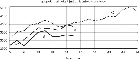
Figure 10 shows PV distributions at 925 hPa and at the 285 K isentropic surface (around the 700–600 hPa level) in the X–Y domain of case A. During the incipient stage of this PL, a cold air dome associated with an upper-level cold vortex approached an incipient disturbance from the top left of the domain (Fig. 10a). This cold air dome was larger than the PL that occurred later. The evolution of geopotential height of case A within the area of the incipient disturbance (Fig. 10, bold rectangle) shows that, in general, the geopotential height of the 285 K isentropic surface gradually increased by ~1000 m until 1500 UTC on 28 December (Fig. 11). At 0600 UTC on 28 December (at 6 hour in Fig. 11), the geopotential height dipped as a result of an increase in the low-level PV together with a decrease in the altitude of the 285 K isentropic surface caused by enhanced convection within the focal area. The horizontal winds on the 285 K isentropic surface in the focal area were relatively weak (Fig. 10a), but horizontal wind shear due to northeasterly and northwesterly winds caused convection (see Fig. 3a) within low-level convergence areas in the focal area (not shown). Then, an initial disturbance without any distinct centre (Fig. 10b) developed by a stretching effect (not shown). These conditions suggest that the incipient disturbance was caused by the ‘vacuum cleaner’ effect (Hoskins et al., 1985) of an upper-level cold vortex.

Fig. 10 Case A. Horizontal cross sections of the X–Y domain at 0300 UTC and 1500 UTC on 28 December and 0000 UTC on 29 December 2006: (a, c, e) at the 285 K isentropic surface, and (b, d, f) at 925 hPa. In panels (a), (c) and (e), PV is shown by blue shading with blue contours at intervals of 1.0 PVU (= 10⁻⁶m² s⁻¹ K kg⁻¹). Black contours and vectors denote geopotential height (every 250 m) and horizontal wind, respectively. In panels (b), (d) and (f), solid contours, dotted contours, vectors and blue shading denote geopotential height (every 25 m), potential temperature (every 2 K), horizontal wind and PV (PVU), respectively. Bold rectangle shows the area of the incipient disturbance of case A. Line AB shows the location of the vertical cross section in Fig. 12.

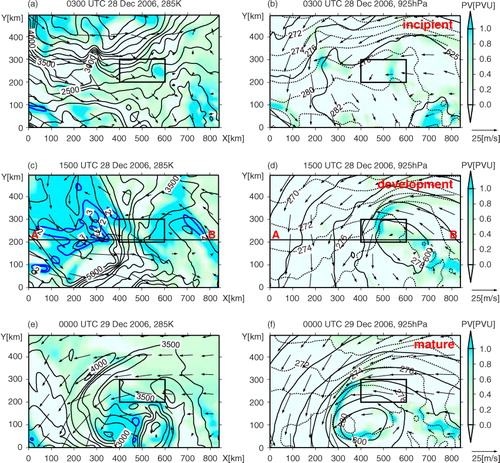
Fig. 11 Time evolution of geopotential height (m) on isentropic surfaces within the enclosed areas (bold rectangles or squares) shown in Fig. 10 (case A), 13 (case B) and 15 (case C). Solid line, case A (285 K isentropic surface); dashed line, case B (288 K); and dotted line, case C (285 K).

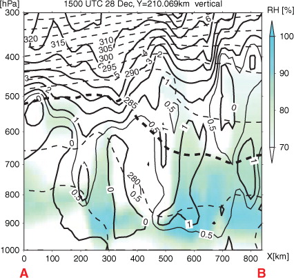
During the development stage, an isolated UPV anomaly accompanied the cold air dome on the left side of the low-level incipient PL (Fig. 10c). In addition, a weak positive PV anomaly moved from the right side of the X–Y domain to the PL. The convection around the PL became further enhanced (see Fig. 3b), and PV anomalies were generated in the low-level atmosphere along the frontal zone (Fig. 10d). A zonal–vertical cross section of PV, potential temperature and relative humidity across the low-level PL (Fig. 12; along the line AB in Fig. 10c and 10d) shows that high PV (around X=200 km), accompanied by dry air, intruded below 700 hPa with a maximum PV of more than 1 PVU on the left side of the low-level PL. For examination of eq. (2), the horizontal scale L of the PV anomaly on the 285 K isentropic surface was ~300 km, was ~280 K, was ~10 K per 3260 m (averaged over the X–Y domain), and ζ _θ on the 285 K isentropic surface averaged over L was ~1.5 f. Using these parameters, we calculated the Rossby height H _R with respect to the PV anomaly to be ~4580 m. Thus, the PV structure was favourable for the development of the PL. The mature stage of the PL was characterised by a PV structure such that PL circulation was maintained by both the UPV anomalies above the PL centre and the lower-level PV anomalies along the frontal zone (Fig. 10e and 10f).

Fig. 12 Case A. Vertical cross section along the line AB shown in Fig. 10c and 10d at 1500 UTC on 28 December 2006: PV (thick contours, every 1.0 PVU), 0.5 PVU PV (thin contours), potential temperature (dashed contours, every 5 K), 285 K potential temperature (bolded dashed contour) and relative humidity (%) (blue shading).

Figure 13 shows PV distributions at 925 hPa and on the 288 K isentropic surface (around the 700–600 hPa level) in the X–Y coordinate domain of case B. During the incipient stage of the PL, geopotential height on the 288 K isentropic surface within the area of the incipient disturbance (Fig. 13, bold rectangle) increased by ~1000 m (Fig. 11). The horizontal wind speed on the 288 K isentropic surface within that area (around 700 hPa) was ~15 m s⁻¹ (Fig. 13a) and that was slower than the speed of the southern part of the eastward moving cold vortex (~25 m s⁻¹, not shown). In the left side of the X–Y domain at around 600 hPa, which corresponded to the south-east quadrant of the vortex, updraft occurred widely (not shown), which possibly led to low-level convergence. In the low-level atmosphere, two incipient disturbances (d1 and d2, Fig. 13b) appeared around the convergence areas of the northeasterly and northwesterly winds, where convection was becoming gradually enhanced (Fig. 5a).

Fig. 13 Case B. Horizontal cross sections of the X–Y domain at 1200 UTC and 2100 UTC on 5 February and at 0300 UTC on 6 February 2008: (a, c, e) at the 288 K isentropic surface; and (b, d, f) at 925 hPa. In panels (a), (c) and (e), PV is shown by blue shading with blue contours at intervals of 1.0 PVU. Black contours and vectors denote geopotential height (every 250 m) and horizontal wind, respectively. In panels (b), (d) and (f), solid contours, dotted contours, vectors and blue shading denote geopotential height (every 25 m), potential temperature (every 2 K), horizontal wind and PV (PVU), respectively. In panel (b) and (d), two incipient disturbances d1 and d2 are also shown. Bold rectangle shows the area of the incipient disturbance d1 of case B.

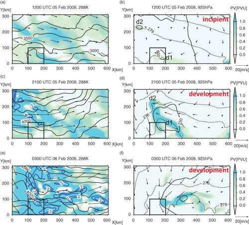
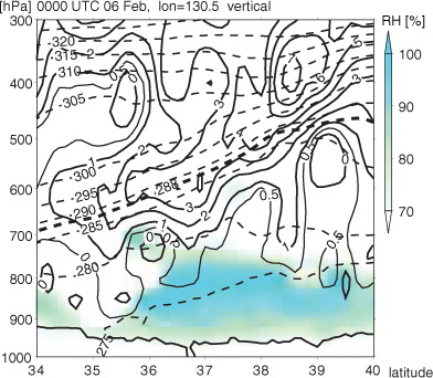
During the development stage, a PV anomaly with a scale of ~300 km was present on the 288 K isentropic surface to the left of the PL (Fig. 13c and 13e). The UPV anomaly gradually decreased (around X=150–400 km and Y=100–200 km in Fig. 13e), except in the area above the PL centre, either because of advection of a negative PV anomaly from lower levels or diabatic heating in the lower levels. A north-south cross section along 130.5°E of PV, potential temperature and relative humidity at 0000 UTC on 6 February (Fig. 14) shows that a PV anomaly (around 36°N) intruded to the 700–600 hPa level. The PV anomaly extended southward and had a shallow structure (from 750 to 500 hPa). Using L on the 288 K isentropic surface ~300 km, ~281 K, ~11 K per 3272 m (averaged over the X–Y domain) and ζ _θ on the 288 K isentropic surface ~1.5 f, we calculated the Rossby height H _R of the PV anomaly to be ~4380 m. The southward extension of the UPV anomaly favoured the development of the southern pre-disturbance d1 (Fig. 13d and 13f).

Fig. 14 Case B. Vertical cross section along 130.5°E (see Fig. 17b) at 0000 UTC on 6 February 2008: PV (thick contours, every 1.0 PVU), 0.5 PVU PV (thin contours), potential temperature (dashed contours, every 5 K), 288 K potential temperature (bold dashed contour) and relative humidity (%) (blue shading).

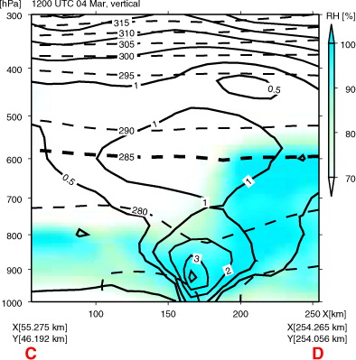
Figure 15 shows the PV distribution at 925 hPa and on the 285 K isentropic surface (at around 600 hPa) in the X–Y coordinate domain of case C. The geopotential height on the 285 K isentropic surface within the area of the incipient disturbance (Fig. 15, bold rectangle) gradually increased by ~1000 m during the first 15 hours of the development stage (Fig. 11). The horizontal winds on the 285 K isentropic surface within that area were relatively weak (not shown). During the development stage, there was a meso-α scale PV anomaly on the 285 K isentropic surface to the left of the low-level PL (Fig. 15a). The vertical cross section of PV, potential temperature and relative humidity (Fig. 16; along the line CD shown in Fig. 15a and 15b) shows that a high PV anomaly (around X=170 km) intruded to ~600 hPa above the PL. Using L on the 285 K isentropic surface ~150 km, ~280 K, ~10 K per 3261 m (averaged over the X–Y domain), ζ _θ on the 285 K isentropic surface ~2 f, we calculated the Rossby height H _R of the PV anomaly to be ~2510 m. It is much smaller than the Rossby heights of cases A and B, primarily because of the smaller size of the PV anomaly. However, the magnitude of the PV anomaly may have been sufficient to affect the lower levels, because the lower the altitude the lower the static stability (Fig. 16).

Fig. 15 Case C. Horizontal cross sections of the X–Y domain at 1200 UTC on 4 March and 0300 UTC on 5 March 2008: (a, c) at the 285 K isentropic surface, and (b, d) at 925 hPa. In panels (a) and (c), PV is shown by blue shading with blue contours at intervals of 1.0 PVU. Black contours and vectors denote geopotential height (every 250 m) and horizontal wind. In panels (b) and (d), solid contours, dotted contours, vectors and blue shading denote geopotential height (every 25 m), potential temperature (every 2 K), horizontal wind and PV (PVU), respectively. Bold rectangle shows the area of the incipient disturbance of case C. Line CD shows the location of the vertical cross section in Fig. 16.

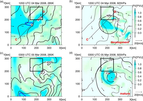
Fig. 16 Case C. Vertical cross section along the line CD in Fig. 15a and 15b at 1200 UTC on 4 March 2008: PV (thick contours, every 1.0 PVU), 0.5 PVU PV (thin contours), potential temperature (dashed contours, every 5 K), 285 K potential temperature (bold dashed contour) and relative humidity (%) (blue shading).

During the mature stage the case C PL decayed gradually (Fig. 8). The PV anomaly around the 285 K isentropic surface moved to the top right side of the X–Y domain (Fig. 15c), whereas the low-level PV anomaly stayed in the centre of the PL (Fig. 15d). These conditions suggest that the UPV anomaly is the driving force of the PL development.

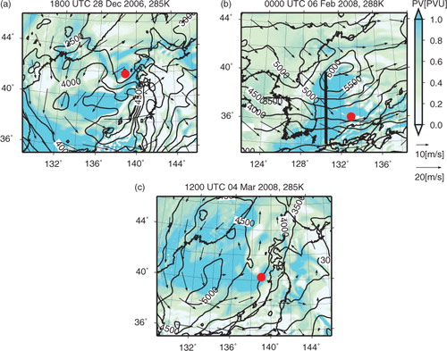
Figure 17 shows PV distributions over a wider area: case A (285 K isentropic surface), case B (288 K) and case C (285 K). Each meso-α scale PV anomaly at around the 700–600 hPa level moving to each PL is a portion of a synoptic-scale PV anomaly associated with an upper-level cold vortex. Each PL was located in a wide region of low static stability associated with a cold vortex. In subsection 5.3, we will discuss what can keep a meso-α scale PL from increasing in size under such a synoptic-scale UPV anomaly, even though meso-α scale disturbances often increase in size and develop into synoptic-scale mid-latitude cyclones.

Fig. 17 Geopotential height (solid contours, every 250 m) and horizontal wind (vectors): (a) case A, 285 K isentropic surface at 1800 UTC on 28 December 2006 (development stage); (b) case B, 288 K isentropic surface at 0000 UTC on 6 February 2008 (development stage); and (c) case C, 285 K isentropic surface at 1200 UTC on 4 March 2008 (development stage). A red circle marks the centre of each PL, and shading indicates isentropic PV. Heavy straight line in (b) shows the location of the vertical cross section in Fig. 14.

4.3. Energy budget analysis

Although in section 4.2 we indicated that a UPV anomaly contributed to the development of all three PLs, the influence of low-level baroclinicity may have differed among the three PLs. Therefore, we conducted potential and kinetic energy budget analyses to examine the role of low-level baroclinicity in the development of each PL.

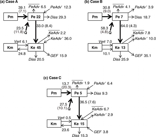
Figure 18 displays the EPE and EKE budgets (eqs. 7 and 8) as energy conversion diagrams. EPE, EKE and each term in eqs. (7) and (8) were averaged horizontally over the X–Y domain over the incipient and development stage of each PL, and vertically from 925 to 800 hPa. Thus, the focus is on PL circulation at and below 800 hPa. EKE increased essentially through [Pe, Ke] from [Pm, Pe] and [Q, Pe], which were the energy sources of the three PLs. The dominant process was baroclinic development ([Pm, Pe]>[Q, Pe]) in case A, whereas diabatic development ([Pm, Pe]<[Q, Pe]) was dominant in cases B and C.

Fig. 18 Flow charts of the energy budgets showing EPE and EKE cycling. The numerals in boxes after Pe or Ke indicate the energy (m² s⁻²) averaged horizontally over each X–Y domain over the incipient and development stage of each PL, and vertically from 925 hPa to 800 hPa. Numerals next to the arrows are energy conversion rates (10⁻⁶ s⁻¹) normalised by the averaged Ke, averaged horizontally over the X–Y domain over the incipient and development stage of each PL, and vertically from 925 hPa to 800 hPa. Numerals in parentheses are the reciprocals of the Ke-normalised energy conversion rates (hour): (a) case A (averaged over the period from 0000 UTC on 28 December to 1800 UTC on 29 December 2006); (b) case B (averaged over the period from 0600 UTC on 5 February to 0600 UTC on 6 February 2008); and (c) case C (averaged over the period from 0600 UTC on 3 March 2008 to 1500 UTC on 4 March 2008).

To understand the relationship between the development processes and the strength of baroclinicity, we further investigated the evolution of [Pm, Pe], [Q, Pe], [Pe, Ke] and baroclinicity between 925 and 800 hPa for the basic field defined by each X–Y coordinate domain in the three PL cases (Fig. 19), based on the study of Yanase and Niino (2007). In cases A and B baroclinicity was initially relatively strong, whereas in case C baroclinicity was relatively weaker throughout the PL's lifetime. In cases A and C baroclinicity gradually weakened with time (to <2.0×10⁻³ s⁻¹ at the end of the lifetime of each), whereas in case B baroclinicity decreased less than in cases A and C. The evolution of EKE and baroclinicity over time indicated that each PL strengthened when baroclinicity was relatively strong (Figs. 4a, 6a, 8a and 19). Moreover, the strength of the baroclinicity was related to the PL's shape. When the baroclinicity was relatively strong (>2.0×10⁻³ s⁻¹), the cloud pattern was comma-shaped (Figs. 3b, 5b–d and 7a). As the baroclinicity weakened with PL development, as occurred in cases A and C, the cloud pattern became spiraliform (Figs. 3c, 3d, 7c and 7d). Also, in case A the dominant process changed from baroclinic into diabatic development (Fig. 19a).

Fig. 19 Time evolution of [Pm, Pe] (dashed line), [Q, Pe] (thin solid line), [Pe,Ke] (dotted line) and baroclinicity (thick solid line with circles) averaged over each X–Y domain. Unlike the values in Fig. 18, these values are not normalised. (a) Case A; (b) case B; (c) case C.

Comparison of the [Pm, Pe]/[Q, Pe] ratio between cases A and C showed that the stronger the baroclinicity, the greater the ratio (Fig. 19a and 19c). If the initial value of the meridional gradient of the basic potential temperature had been maintained throughout the lifetime of case C, [Pm, Pe]/[Q, Pe] would be greater, although [Q, Pe] and the meridional eddy heat transport, would also increase because of enhanced frontal convection and increased EKE, respectively. However, comparison of the energy sources between cases A and B showed that the dominant processes differed, even though baroclinicity was almost the same during the first half of the lifetime of each (Fig. 19a and 19b). One reason for this was the relatively high EKE of case A, which caused the relatively high [Pm, Pe] through . In addition, in case B, [Pm, Pe] rapidly decreased because was negative in broad areas of the X–Y domain while the dissipating pre-disturbance d2 (at around X=120 km and Y=200 km in Fig. 13d) was moving south-eastward. This SE-ward motion was due to strong northerly winds on the left side of the X–Y domain. As a result, overall EKE decreased (Fig. 6a) and the baroclinicity did not decrease to less than 2.0×10⁻³ s⁻¹ until the end of the PL's lifetime (Fig. 19b). The magnitude of [Q, Pe] differed between cases B and C (Fig. 19b and 19c), even though the magnitude of EKE was almost the same between them (Figs. 6a and 8a). In case B, stronger baroclinicity (Figs. 9b, Figs. 9c, 19b and 19c) caused convection to be stronger (e.g. Figs. 5c and Figs. 7b), resulting in lower and higher from 925 hPa to 800 hPa in the ninth term on the rhs of eq. (7).

The low-level baroclinicity was an important factor in the development of the PLs. However, the manifestation of that factor depended on the magnitude of EKE and on the presence of specific structures, as in case B.

5. Discussion

5.1. Processes influenced by a UPV anomaly

Processes that were influenced by a UPV anomaly were likely associated with the development of all three PLs. To demonstrate the effect of PV anomalies at around 600 hPa on PL development at lower levels, we use the Rossby radius of deformation (Van Delden et al., 2003). The Rossby radius of deformation is calculated by9 where H is the vertical scale. In the case of this study, when the PLs developed, typical values of N and H were ~10⁻² s ⁻¹ and ~4000 m, respectively. By substituting these values into eq. (9), we obtain for λ _RI a value of ~400 km. This value is reasonable in comparison with the PL scale as described in subsection 4.2. If PV anomalies above 600 hPa contributed directly to the development of PLs at lower levels, then values of N and H would be higher, and the value of λ _RI would also be larger than the PL scale (<1000 km).

5.2. Baroclinic interaction between upper- and lower-level disturbances

In order to further clarify the characteristics of an upper-level cold vortex and baroclinic development, we investigated the baroclinic interaction between each low-level PL and the upper-level disturbance. Here, we examined whether the features of baroclinic development in the PLs are similar to those in typical extratropical cyclones, in which, in general, upper and lower disturbances interact and intensify together. According to Hoskins et al. (1985), such baroclinic development in the extratropical cyclones requires a horizontal gradient of the zonal mean PV in the meridional direction.

No horizontal gradient of the zonal mean PV existed continuously along the Y (meridional) direction on the upper-level isentropic surfaces in any of the three PL cases, although near the surface, horizontal gradient of potential temperature, which is identical to the PV gradient, existed (e.g. Figs. 10 and 13 and 15). When the PL developed, the upper-level disturbance associated with the meso-α scale UPV anomaly showed no development at all, but just passed over the low-level PL. This is likely because the mobile UPV anomaly becomes cut off and cannot be increased by the advection of high PV (Figs. 10c, 13e, 15a and 17). In addition, the case C PL completed its development just before the UPV anomaly passed north-eastward over the lower-level PL. These features differ from those in the development of the typical extratropical cyclones as described above. This is a common characteristic of PLs that develop in association with a cold vortex and an isolated PV anomaly, at least for three cases in this study. This finding might be contrary to previous studies that concluded that PL development is caused by baroclinic instability (Grønås and Kvamstø, 1995; Rasmussen et al., 1996; Claud et al., 2004), even though the PV distributions were almost the same as those in this study. Montgomery and Farrell (1992) hypothesised that the development mechanisms of PLs were the same as those of mid-latitude cyclones. However, our results here differ from those of Montgomery and Farrell (1992), partly because we examined actual PLs accompanied by a cut-off cold vortex, whereas Montgomery and Farrell (1992) studied the PL development mechanism using idealised numerical experiments that did not consider the presence of a cut-off cold vortex.

5.3. Favourable conditions for PL development

Our PV analysis results suggested that at least two conditions are needed for PL development: a meso-α scale PV anomaly intruding to the 700–600 hPa level (condition I) and low static stability in the lower troposphere (condition II). These two conditions correspond to the two parameters, marine cold-air outbreaks associated with low-level static stability and tropopause level as an indicator of upper-level forcing, assessed by Kolstad (2011). Also, these two conditions may correspond to the condition proposed by Grønås and Kvamstø (1995), namely, a height difference of less than 1000 m between the tropopause, defined as the 2 PVU surface, and the top of the convective mixing layer below. Yanase et al. (2004) indicated that turbulent heat fluxes from the sea surface played a role in the maintenance of low static stability below altitudes of 1 km. Considering this finding, an upper-level cold vortex contributes to realising conditions I and II over the warm ocean.

The results of our energy budget analysis indicated that a third condition, low-level baroclinicity (condition III), is also necessary for PL development. Under relatively strong baroclinicity in the low-level atmosphere, PLs can efficiently develop through energy supplied as [Q, Pe], via the formation of strong mesoscale fronts and convection, as well as through [Pm, Pe]. An important role of [Q, Pe] in PL development is consistent with the results of previous numerical experiments. For example, Lee et al. (1998) have reported that a PL accompanied by an upper-level cold vortex showed little development in case that condensational heating was switched off in their numerical simulations. According to the results of idealised numerical experiments performed by Yanase and Niino (2007), an idealised PL can develop under the initial conditions of no baroclinicity and no UPV anomaly, but the development takes more than 70 hours. However, such environmental conditions do not actually occur poleward of the mid-latitude baroclinic zone. Although baroclinic environment may generally lead to a comma-shaped cloud pattern, we also found that the PL cloud pattern changed to spiraliform as the baroclinicity weakened. Nordeng and Rasmussen (1992), in fact, have reported that a PL with a spiraliform cloud pattern observed in the Barents Sea had a comma-shaped cloud pattern at an early stage of development.

In addition to these three conditions, one more condition may be needed for a PL to remain meso-α scale under the existence of a synoptic-scale UPV anomaly, by which synoptic-scale cyclonic circulation can be induced at lower levels. This induced circulation can cause synoptic-scale warm advection in the front of the cold vortex, which can lead to the formation of a synoptic-scale mid-latitude cyclone. In fact, a mid-latitude synoptic-scale cyclone often develops accompanied by a synoptic-scale, upper-level, cut-off low. If there existed synoptic-scale warm advection induced by the UPV anomaly on the eastern flank of a meso-α scale PL, the PL would increase in size, resulting to a synoptic-scale low. Considering this, we speculate that for a meso-α scale PL to remain its size, low-level synoptic-scale cold advection is needed to cancel out the synoptic-scale warm advection induced by the UPV anomaly. Wu et al. (2011) showed in their piecewise PV diagnosis of PL development that cold advection by a synoptic-scale mid-latitude cyclone on the eastern flank of a PL exceeded warm advection induced by a UPV anomaly. Thus, we propose that synoptic-scale cold advection in the low-level atmosphere is a fourth condition (condition IV) necessary for a PL to remain meso-α scale. This condition is implied in the definition of PLs proposed by Turner et al. (2003), who indicate that a PL ‘forms poleward of the main baroclinic zone’. All three cases studied here met this condition (see Fig. 1b–d).

Besides these four conditions, a reverse-shear condition is also known to be favourable for PL (e.g. Kolstad, 2006). Kolstad (2006) defined the criteria related to reverse thermal shear and low static stability for reverse shear PLs and showed several areas where such conditions occur with high frequency. All three PL cases studied here met such conditions when the PLs were incipient disturbances (not shown). A reverse shear flow condition may be realised with both the condition III and IV in the Sea of Japan.

In the Sea of Japan, warm SSTs are distributed parallel to the coastline of Japan, and cold SSTs are distributed on the opposite side (Fig. 1a). With northerly winds (cold advection), these SST distributions favour the formation of low-level baroclinicity with reverse shear flow. Therefore, in the Sea of Japan, the four conditions (I–IV) are met simultaneously when moderate cold advection occurs in the low-level atmosphere and an upper-level cold vortex exists. Whether these four conditions inevitably lead to the development of a PL, and whether there may be additional necessary conditions, should be addressed in future studies.

6. Summary and conclusions

Previous studies have reported that PLs over the Sea of Japan develop under low-level baroclinicity in connection with the approach of an upper-level cold vortex. However, the relationship between a synoptic-scale upper-level cold vortex and a meso-α scale PL, and the role played by low-level baroclinicity in the development of the PL have not been well investigated. We therefore examined three PL cases over the Sea of Japan to clarify their development processes, in particular from the perspective of PV and energy budgets. We used meso-analysis data with a horizontal resolution of approximately 11 km provided by the JMA. For a comprehensive understanding of various types of PLs over the Sea of Japan, it was very useful to compare three PLs based on the same analyses. Table 1 summarises the results of our analyses. Several findings regarding PLs over the Sea of Japan were obtained from this study: the roles of a synoptic-scale cold vortex accompanied by a cold dome and the different scales of UPV anomalies, the importance of low-level baroclinicity in diabatic processes, and no development of an upper-level disturbance associated with a UPV anomaly.

Table 1. Characteristics of the three PLs of cases A, B and C

Case	A	B	C
Rossby height, H R	4580 m	4380 m	2510 m
Scale of the intruding UPV anomaly, L	300 km	300 km	150 km
Location of the cold vortex at 500 hPa during the mature stage	Immediately above the PL	400 km north of the PL	Immediately above the PL
Baroclinicity	Strong→weak	Strong	Strong→weak
Cloud pattern	Comma-shaped→spiraliform	Comma-shaped	Comma-shaped→spiraliform
Dominant development process	Baroclinic	Diabatic	Diabatic
Magnitude of EKE	Large	Small	Small

First, we showed that each of the three PLs had a distinct mesoscale frontal structure. This front was accompanied by active convection, irrespective of whether the cloud patterns were comma-shaped or spiraliform.

Then, we performed a PV analysis to examine the roles played by the upper-level cold vortex and the associated PV anomaly in PL development. The results indicated that with the approach of a synoptic-scale cold air dome, the geopotential height of the upper-level isentropic surfaces in the front of the cold vortex increased by ~1000 m. At that time, convections enhanced and an incipient disturbance occurred. These situations suggested the ‘vacuum cleaner’ effect (Hoskins et al., 1985) by a cold vortex on the occurrence of an incipient disturbance, a possibility that should be examined in detail in future work. When the incipient disturbance developed into a meso-α scale PL, a meso-α scale UPV anomaly, which intruded to around the 700–600 hPa level and which is just a part of a synoptic-scale PV anomaly accompanying the cold vortex, moved to the west side of the low-level PL. The PL was located in the wide region of low static stability in the lower troposphere within the cold dome. Low static stability can be caused by the presence of a cold dome over the warm ocean (e.g. Yanase et al., 2004). The large value of the Rossby height and the location of the meso-α scale UPV anomaly were favourable for the development of the PLs by upper-level forcing. These conditions suggested that a synoptic-scale cold vortex played a role in creating a favourable environment for PL development.

In the low-level atmosphere, the PL developed under the influence of both the UPV anomaly and low-level PV anomalies generated by diabatic heating along the frontal zone. In contrast, the upper-level disturbance associated with the meso-α scale UPV anomaly shows no development at all. These features differ from those in the development of typical extratropical cyclones, in which, in general, upper and lower disturbances interact and intensify together. This is likely because of the mobile UPV anomaly cut off from its source. Under such a synoptic-scale UPV anomaly, for the developed PL over the Sea of Japan to remain meso-α scale, we proposed that synoptic-scale cold advection in the low-level atmosphere is needed.

To clarify the role of low-level baroclinicity in PL development, we investigated the relationship between baroclinicity strength and PL shape. When baroclinicity was relatively strong, the PL cloud pattern was comma-shaped. As the baroclinicity weakened, in cases A and C, the cloud pattern gradually became spiraliform. The energy budget analysis indicated that low-level baroclinicity was an important factor in differentiating the energy sources necessary for PL development. When baroclinicity was strong, the conversion of energy from mean available potential energy to eddy available potential energy ([Pm, Pe]) dominated. These results are consistent with the results of idealised numerical experiments by Yanase and Niino (2007). In addition, in our actual PL examples, EKE increased when low-level baroclinicity was relatively strong. The strength of baroclinicity, through its enhancement of mesoscale fronts and convection, affected the amount of energy generated by diabatic heating ([Q, Pe]), as well as the amount provided by [Pm, Pe]. Under very weak baroclinicity, frontal activity would be weak, and PLs would not be assured an energy supply sufficient for their development. Therefore, we suggest that strong baroclinicity is necessary for PL development, even though diabatic development is dominant. Through these results, we also verified that the energy budget analysis using a carefully specified X–Y coordinate system was valid for a PL study.

Based on our results and discussions, we propose that at least four conditions are necessary for the development of meso-α scale PLs: a meso-α scale PV anomaly intruding to the 700–600 hPa level (condition I), low static stability in the low-level atmosphere (condition II), strong baroclinicity in the low-level atmosphere (condition III) and synoptic-scale cold advection in the low-level atmosphere (condition IV). In the Sea of Japan, they are met simultaneously when an upper-level cold vortex approaches the area above an area of synoptic-scale cold advection in the low-level atmosphere. In such environment, it is possible for a meso-α scale PL to develop in association with a mesoscale front.

This study suggested that a cold vortex is a key to PL development, including three processes: decreasing static stability, inducing low-level circulation leading to baroclinic development by a meso-α scale UPV anomaly and the possibility of the occurrence of an incipient disturbance in the front of the cold vortex. For better understanding of PLs, it is necessary to quantify these processes in a future study. We believe that the results of the present study provide a basis for future studies addressing these issues.

7. Acknowledgements

This paper is a part of a master's thesis submitted to the Graduate School of Environment Science, Hokkaido University, in March 2009. U. Shimada is deeply grateful to Prof. Y. Fujiyoshi, Prof. A. Kubokawa and Dr. M. Kawashima of Hokkaido University for helpful discussions. The authors thank two anonymous reviewers for valuable comments that have greatly improved the manuscript. This work was supported by MEXT KAKENHI Grant Number 25106708 and partly supported by the Green Network of Excellence Program (GRENE Program) Arctic Climate Change Research Project.

References

- Asai T . Meso-scale features of heavy snowfalls in Japan Sea coastal regions of Japan. (in Japanese). Tenki. 1988; 35: 156–161.
- Asai T. , Miura Y . An analytical study of meso-scale vortex-like disturbances observed around Wakes Bay area. J. Meteorol. Soc. Japan. 1981; 59: 832–843.
- Bracegirdle T. J. , Gray S. L . The dynamics of a polar low assessed using potential vorticity inversion. Q. J. Roy. Meteorol. Soc. 2009; 135: 880–893.
- Bresch J. F. , Reed R. J. , Albright M. D . A polar-low development over the Bering Sea: analysis, numerical simulation, and sensitivity experiments. Mon. Wea. Rev. 1997; 125: 3109–3130.
- Claud C. , Heinemann G. , Raustein E. , Mcmurdie L . Polar low le Cygne: satellite observations and numerical simulations. Q. J. Roy. Meteorol. Soc. 2004; 130: 1075–1102.
- Craig G. C. , Cho H. R . Cumulus heating CISK in the extratropical atmosphere Part I: polar lows and comma clouds. J. Atmos. Sci. 1988; 45: 2622–2640.
- Craig G. C. , Gray S. L . CISK or WISHE as the mechanism for tropical cyclone intensification. J. Atmos. Sci. 1996; 53: 3528–3540.
- Duncan C. N . A numerical investigation of polar lows. Q. J. Roy. Meteorol. Soc. 1977; 103: 255–267.
- Emanuel K. A. , Fantini M. , Thorpe A. J . Baroclinic instability in an environment of small stability to slantwise moist convection. Part I: two-dimensional models. J. Atmos. Sci. 1987; 44: 1559–1573.
- Emanuel K. A. , Rotunno R . Polar lows as arctic hurricanes. Tellus A. 1989; 41: 1–17.
- Føre I. , Kristjánsson J. E. , Kolstad E. W. , Bracegirdle T. J. , Saetra Ø. , co-authors . A ‘hurricane-like’ polar low fuelled by sensible heat flux: high-resolution numerical simulations. Q. J. Roy. Meteorol. Soc. 2012; 138: 1308–1324.
- Føre I. , Nordeng T. E . A polar low observed the Norwegian Sea on 3–4 March 2008: high-resolution numerical experiments. Q. J. Roy. Meteorol. Soc. 2012; 138: 1983–1998.
- Fu G. , Niino H. , Kimura R. , Kato T . A polar low over the Japan Sea on 21 January 1997. Part I: observational analysis. Mon. Wea. Rev. 2004; 132: 793–814.
- Grønås S. , Kvamstø N. G . Numerical simulations of the synoptic conditions and development of Arctic outbreak polar lows. Tellus A. 1995; 47: 797–814.
- Hewson T. D. , Craig G. C. , Claud C . Evolution and mesoscale structure of a polar low outbreak. Q. J. Roy. Meteorol. Soc. 2000; 126: 1031–1063.
- Hoskins B. J. , McIntyre M. E. , Robertson A. W . On the use and significance of isentropic potential vorticity maps. Q. J. Roy. Meteorol. Soc. 1985; 111: 877–946.
- Kolstad E. W . A new climatology of favourable conditions for reverse-shear polar lows. Tellus A. 2006; 58: 344–354.
- Kolstad E. W . A global climatology of favourable conditions for polar lows. Q. J. Roy. Meteorol. Soc. 2011; 137: 1749–1761.
- Kurihara Y. , Sakurai T. , Kuragano T . Global daily sea surface temperature analysis using data from satellite microwave radiometer, satellite infrared radiometer and in-situ observations. (in Japanese). Wea. Bull. JMA. 2006; 73: s1–s18.
- Lee T. Y. , Park Y. Y. , Lin Y. L . A numerical modeling study of mesoscale cyclogenesis to the east of the Korean peninsula. Mon. Wea. Rev. 1998; 126: 2305–2329.
- Mailhot J. , Hanley D. , Bilodeau B. , Hertzman O . A numerical case study of a polar low in the Labrador Sea. Tellus A. 1996; 48: 383–402.
- Mansfield D. A . Polar lows: the development of baroclinic disturbances in cold air outbreaks. Q. J. Roy. Meteorol. Soc. 1974; 100: 541–554.
- Montgomery M. T. , Farrell B. F . Polar low dynamics. J. Atmos. Sci. 1992; 49: 2484–2505.
- Ninomiya K. , Hoshino K . Evolution process and multi-scale structure of a polar low developed over the Japan Sea on 11–12 December 1985. Part II: meso-β-scale low in meso-α-scale polar low. J. Meteorol. Soc. Japan. 1990; 68: 307–318.
- Ninomiya K. , Hoshino K. , Kurihara K . Evolution process and multi-scale structure of a polar low developed over the Japan Sea on 11–12 December 1985. Part I: evolution process and meso-α-scale structure. J. Meteorol. Soc. Japan. 1990; 68: 293–306.
- Nordeng T. E. , Rasmussen E. A . A most beautiful polar low. A case study of a polar low development in the Bear Island region. Tellus A. 1992; 44: 81–99.
- Rasmussen E . The polar low as an extratropical CISK disturbance. Q. J. Roy. Meteor. Soc. 1979; 105: 531–549.
- Rasmussen E. A. , Claud C. , Purdom J . Labrador Sea polar lows. Global Atmos. Ocean. Sys. 1996; 4: 275–333.
- Reed R. J. , Duncan C. N . Baroclinic instability as a mechanism for the serial development of polar lows: a case study. Tellus A. 1987; 39: 376–385.
- Saito K. , Fujita T. , Yamada Y. , Ishida J. , Kumagai Y. , co-authors . The operational JMA nonhydrostatic mesoscale model. Mon. Wea. Rev. 2006; 134: 1266–1298.
- Sardie J. M. , Warner T. T . On the mechanism for the development of polar lows. J. Atmos. Sci. 1983; 40: 869–881.
- Shapiro M. A. , Fedor L. S. , Hampel T . Research aircraft measurements of a polar low over the Norwegian Sea. Tellus A. 1987; 39: 272–306.
- Shapiro M. A. , Keyser D . Newton C. W. , Holopainen E. O . Fronts, jet streams and the tropopause. Extratropical Cyclones. 1990; Boston, USA: American Meteorological Society. 167–191. The Eric Palmen Memorial Volume.
- Tsuboki K. , Wakahama G . Mesoscale cyclogenesis in winter monsoon air streams: quasi-geostrophic baroclinic instability as a mechanism of the cyclogenesis off the west coast of Hokkaido Island. Japan. J. Meteorol. Soc. Japan. 1992; 70: 77–93.
- Turner J. , Rasmussen E. A. , Carleton A. M . Rasmussen E. A. , Turner J . Introduction. Polar Lows: Mesoscale Weather Systems in the Polar Regions. 2003; Cambridge, UK: Cambridge University Press. 1–51.
- Van Delden A. , Rasmussen E. A. , Turner J. , Røsting B . Rasmussen E. A., Turner J . Theoretical investigations. Polar Lows: Mesoscale Weather Systems in the Polar Regions. 2003; Cambridge, UK: Cambridge University Press. 286–404.
- Wu L. T. , Martin J. E. , Petty G. W . Piecewise potential vorticity diagnosis of the development of a polar low over the Sea of Japan. Tellus A. 2011; 63: 198–211.
- Yamagishi Y. , Doi M. , Kitabatake N. , Kamiguchi H . A polar low which accompanied strong gust. (in Japanese). Tenki. 1992; 39: 27–36.
- Yanase W. , Fu G. , Niino H. , Kato T . A polar low over the Japan Sea on 21 January 1997. Part II: a numerical study. Mon. Wea. Rev. 2004; 132: 1552–1574.
- Yanase W. , Niino H . Dependence of polar low development on baroclinicity and physical processes: an idealized high-resolution numerical experiment. J. Atmos. Sci. 2007; 64: 3044–3067.
- Yarnal B. , Henderson K. G . A climatology of polar low cyclogenetic regions over the North Pacific Ocean. J. Clim. 1989; 2: 1476–1491.