A novel method to improve temperature simulations of general circulation models based on ensemble empirical mode decomposition and its application to multi-model ensembles

Abstract

A novel method based on the ensemble empirical mode decomposition (EEMD) method was developed to improve model performance. This method was evaluated by applying it to global surface air temperatures, which were simulated by eight general circulation models from the Coupled Model Intercomparison Project Phase 5 (CMIP5). The temperature simulations of the eight models were separated into their different components by EEMD. The model's performance improved after the first high-frequency component was removed from the original simulations by EEMD for each model, on both the global and continental scale. Moreover, EEMD was more effective in improving the model's performance compared to the wavelet transform method. The multi-model ensembles (MMEs) were calculated based on the EEMD-improved model simulations using the Average Ensemble Mean, Multiple Linear Regression, Singular Value Decomposition and Bayesian Model Averaging methods. The results showed that the MME forecasts performed better when the calculations were based on the EEMD-improved simulations as opposed to the original simulations on both the global and continental scale. Therefore, the results of the MME were further improved by using the EEMD-improved model simulations. This new method provides a simple way to improve model performance and can be easily applied to further improve MME simulations.

• EEMD
• multi-model ensemble
• CMIP5

1. Introduction

Atmosphere–Ocean General Circulation Models (AOGCMs) are powerful tools that can enhance our understanding of climate variability and project future climate changes. A number of AOGCMs have been used to simulate past climate changes between 1850 and 2005, and to predict future climate changes from 2006 to 2100 under different scenarios. However, it is very difficult to identify the most reliable model simulation as different AOGCMs have different performance levels in different regions (Giorgi and Mearns, 2003; Chen et al., 2006). In general, a good agreement with past simulations builds confidence in the reliability of future projections (Reifen and Toumi, 2009). Consequently, improving the precision of past simulations by post-processing of model simulations is crucial for future predictions.

Climate model evaluation methods are based on conventional statistics, including correlation and the distance between the simulated and observed data. The most commonly used conventional statistics are correlation, bias and Root Mean Square Error (RMSE). Correlation indicates similarity in variation, while bias and RMSE evaluate the distance between the simulated and observed data. A model has better performance when its simulation has higher correlation, lower bias, and lower RMSE with the observed data than other models.

Multi-model ensemble (MME) methods have been the traditional approach to improving model simulations. After assembling the model results based on MME methods, MME simulations produce more accurate results than any single model (Gates et al., 1999; Doblas Reyes et al., 2005; Hagedorn et al., 2005; Weisheimer et al., 2005,2009; Weigel et al., 2008; Annan and Hargreaves, 2010; Semenov and Stratonovitch, 2010). MME methods include the arithmetic ensemble mean (AEM) and weighted ensemble mean methods. The AEM performs better than any individual model as it integrates the simulated values of multi-models and reduces the simulated error by partly offsetting positive and negative biases of different models. However, the level of improvement achieved by using the AEM has potential problems since there are no guarantees that the errors shared by the models will cancel out (Reifen and Toumi, 2009). Weighted ensemble mean methods are based on the concept that greater weight is given to models that perform better during the training period. Methods such as Multiple Linear Regression (Krishnamurti et al., 1999, 2000; Kharin and Zwiers, 2002; Shin and Krishnamurti, 2003), Singular Value Decomposition (SVD, Feddersen et al., 1999; Yun et al., 2003), reliability ensemble averaging (REA, Giorgi and Mearns, 2002, 2003), and Bayesian Model Averaging (BMA, Raftery et al., 2005; Min and Hense, 2006a, 2006b; Berliner and Kim, 2008) have been shown to produce more accurate results than the AEM when simulating past climate conditions.

Uncertainties in models, which include the initial conditions, boundary conditions, parameter and structural uncertainties (Tebaldi and Knutti, 2007), cause errors between model simulations and observations (Collins et al., 2011). These errors are present in all the components of model simulations, when the model simulations are separated into their different components. However, most errors are contained in certain high-frequency components because the long-term observed trend is well simulated by AOGCMs (IPCC, 2007). Hence, these errors could be reduced if the components containing the most errors are removed from the original simulations, and this represents a novel way to improve model performance. The model's simulations are non-stationary series because they contain the long-term trend. Ensemble Empirical Mode Decomposition (EEMD) is a method to decompose non-stationary signals into different modes. It has previously been proven to be effective in climatic research (Huang and Wu, 2008; Wu et al., 2008; Qian et al., 2009; Franzke, 2010; Breaker and Ruzmaikin, 2011). The model performance would be improved following the removal of the unrelated component. Furthermore, this improvement in model simulations could also be used in MMEs to improve ensemble forecasts. Accordingly, the main goals of this study were: (1) to present improvements in temperature simulations of GCMs with the new method, which was developed based on EEMD; and (2) to apply the EEMD-improved model simulations to improve the MMEs and evaluate them using conventional statistics.

2. Data and method

2.1. Climate data

Global monthly mean temperature data simulated by eight different AOGCMs (Table 1) between 1901 and 2100 were retrieved from the Coupled Model Intercomparison Project Phase 5 (CMIP5) website (http://www-pcmdi.llnl.gov/ipcc/about_ipcc.php), where a more detailed explanation of each model can also be found. Since there is no consistency in the number of ensemble members among the models and only one simulation is available for some models, model outputs from CMIP5 historical r1i1p1 (one ensemble member per model) were used in this study. Monthly observation data of global mean surface air temperature over land were obtained from the Climate Research Unit (CRU) TS 3.0 dataset (www.cru.uea.ac.uk) on a 1°×1° resolution. Because the temperatures simulated by different models had different resolutions, the model data were interpolated to 1°×1° resolution using bilinear interpolation and masked with the observed grid prior to analysis. The anomalies of annual mean temperatures were calculated for the observation and the model simulations.

Table 1. Brief description of the eight GCMs

Model name	Resolution	Country/Institute
BCC-CSM1-1 (BCC)	1.875°×1.875°	China/BCC
CanESM2 (CAN)	2.0°×2.0°	Canada/CCCMA
CNRM-CM5 (CNRM)	2.8°×2.8°	France/CNRM
GISS-E2-H (GISSH)	4.0°×5.0°	American/GISS
GISS-E2-R (GISSR)	5.0°×4.0°	American/GISS
INM-CM4 (INM)	5.0°×4.0°	Russia/INM
IPSL-CM5A-LR (IPSL)	3.75°×2.5°	France/IPSL
NorESM1-M (NOR)	3.75°×3.75°	Norway/NCC

2.2. Empirical ensemble mode decomposition

Huang et al. (1998) developed the Empirical Mode Decomposition (EMD) method. EMD is a general signal processing method used for analysing nonlinear and non-stationary time series. It is an adaptive, data-driven and highly efficient algorithm used to decompose a time series into its intrinsic modes of oscillation. The central idea of EMD is to decompose a time series F(t) into a finite and often small number of intrinsic mode functions (IMFs),1 where n is the number of IMFs; r _n is the residue of the time series x(t). IMF is defined as any function having an equal number of extreme and zero-crossings (or differing at most by one), and also having symmetric envelopes defined by the local minima and maxima, respectively.

The procedure of EMD is implemented through a sifting process: (1) Identify all of the local extremes in the time series F(t) and connect all of the local maxima and minima with a cubic spline as the upper (lower) envelope. (2) Calculate the difference between the data F(t) and the local mean of upper and lower envelopes as the first component h ₁ . (3) Treat h ₁ as the data and repeat steps (1) and (2) until the upper and lower envelopes are symmetric with respect to zero mean under certain criteria. Then, the final h _1j is designated as IMF ₁ . (4) The rest of the data r ₁ =F(t)−IMF ₁ . Treat r ₁ as new data F(t) and repeat steps (1), (2) and (3). The sifting process is completed when the residue r _n becomes a monotonic function. More details of the EMD method can be found in the works of Huang et al. (1998, 1999).

However, EMD suffers from weaknesses, such as the frequent appearance of mode mixing. In an attempt to address these issues, Wu and Huang (2009) introduced the Ensemble EMD (EEMD) method to alleviate some of the common problems of EMD such as mode mixing and increasing robustness of EMD. EEMD was estimated by averaging numerous EMD runs with the addition of some Gaussian noise. By averaging the different decompositions, the noise was averaged out and an estimate of the true decomposition was calculated with a confidence estimate. Using the EEMD algorithm, the signal could be decomposed into its intrinsic modes of oscillation.

The standard deviation of added noise and the ensemble number of EMD were parameters in the EEMD procedure. The sensitivity of the decomposition of data to the amplitude of noise is often small within a certain window of noise amplitude (Wu et al., 2007; Wu and Huang, 2009). Therefore, noise with a standard deviation of 0.2 was added. The ensemble size was set at 1000 in every run to ensure the stability of results.

2.3. Wavelets transform method (WTM)

Wavelets are functions that satisfy certain mathematical requirements that decompose the signals into different frequency components, so that each component can be analysed with a resolution matched to its scale. In terms of some elementary wavelet functions W _f (a,b), wavelet transform decomposes a signal F(t) derived from a ‘mother wavelet’ ω(t) by dilation and translation,2 where W _f (a,b) is the wavelet coefficients; ω _ab is the mother wavelet; a is scale factor (dilation); b is position factor (translation); F(t) is the signal (models’ projections in this study), where in t is time.

Based on the wavelet prototype function called the mother wavelet, an original signal is decomposed into approximate and detailed coefficients by the wavelet transform (Graps, 1995). Approximate coefficients are obtained with a low-frequency version of the mother wavelet while detailed coefficients are obtained with a high-frequency version of the same wavelet (S=Ca ₁ +Cd ₁ =Ca ₂ +Cd ₂ +Cd ₁ =Ca _n +Cd _n +…+Cd ₁ , where S represents the original signal, Ca ₁ , Ca ₂ ,…, Ca _n represents different approximate coefficients, Cd ₁ , Cd ₂ , Cd ₃ ,…, Cd _n represents different detailed coefficients). The low- and high-frequency signals are reconstructed based on approximate and detailed coefficients, respectively. Thus, wavelet transform can decompose a signal into high- and low-frequency signals (S=a ₁ +d ₁ =a ₂ +d ₂ +d ₁ =a _n +d _n +…+d ₁ , where a _1, a _2, … _, a _n represents different low frequency signals, d _1, d _2, … _, d _n represents different high frequency signals).

Several groups of functions can be used as mother wavelets, all of which were tested because the decomposed results depended on the mother wavelet. The best results were obtained using the Daubechies wavelet with three vanishing moments (Db3, Daubechies, 1988, 1992). Thus, the original signals were transformed by wavelet function Db3 in the current study.

2.4. Improvement in MME simulations

In this study, the temperature simulation could be improved by the EEMD method for every model. Then, MME simulations, calculated using the EEMD-improved model simulations, were compared with the MME simulations, which were calculated using the original model simulations to investigate whether MME simulations were also improved. The MME methods used in this research were the AEM, the Multiple Linear Regression method, SVD, and BMA, which are simple but commonly used in MME simulations. Brief descriptions of the MME methods are provided below:

AEM

AEM

The AEM is defined by

3

where Y(t) is an MME projection for time t, N is the total number of AOGCMs, and F _k (t) is a projection of the kth model for time t.

Multiple Linear Regression (Linear)

This method is defined as4 where Y(t) is an MME projection for time t, F _k (t) is a projection of the kth model for time t, a ₀ is a constant, and a _k is a weight for model k. The coefficients a ₀ and a _k are calculated using a multiple regression method (Krishnamurti et al., 1999, 2000).

SVD

The SVD method is defined as5 where Y(t) is an MME prediction for time t, F _k (t) is a forecast of the kth model for time t, and a _k is a weight for model k. The coefficient a _k is calculated using the SVD method to solve the regression function between the model simulations and the observed data. More details of the SVD algorithm for obtaining the coefficient can be found in the study by Yun et al. (2003).  BMA (Bayesian)

The forecast probability density function (PDF) p(y) by BMA is given as6 where w _k is the weight of the kth model and p _k (y∣x _k ) is the forecast PDF based on predictor x _k . The p _k (y∣x _k ) is the conditional PDF and is approximated by a normal distribution centred at a linear function of the predictor, a _k +b _k x _k . Therefore, the BMA mean is the conditional expectation of y given the forecast. Thus, the deterministic BMA ensemble prediction is calculated as7 where a _k and b _k can be obtained by the regression between the x _k and y in the training period. The weights w _k are calculated using the Expectation–Maximization (EM) algorithm. Details of the EM algorithm can be found in Raftery et al. (2005) and Duan et al. (2007).

3. Results

3.1. Decomposition of model simulations by EEMD and WTM

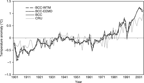
Both global averaged annual observed data (CRU data) and temperature series simulated by eight AOGCMs from 1901 to 2005 were decomposed using EEMD. Each temperature series was decomposed to six IMFs (components). Different IMFs reflected the variations in different frequencies. As the simulations were decomposed by the filter methods in the same way for every model, only the results of the BCC-CSM1-1 model (BCC is a model developed by the Beijing Climate Center) are used as an example in this paper. The IMFs of BCC and the observed data (CRU) are shown in Fig. 1. Each IMF stands for the variation of frequencies at certain timescales. The correlations between the corresponding IMFs of CRU and BCC were calculated (Fig. 1). B1 (IMF1 of BCC) did not correlate well with C1 (IMF1 of CRU), while other IMFs of BCC were highly correlated with their corresponding IMFs of CRU. Thus, B1 was removed from the original BCC simulations. After the removal of B1, the statistical correlation between BCC and CRU improved. Therefore, the IMF1 component was removed from the model simulation to improve the model's performance. Although IMF1 was removed, the filtered series was similar to the original simulations and large differences between the model simulation and CRU were smoothed (Fig. 2). The simulated and observed temperatures were also decomposed by WTM. The optimal results were also obtained by removing the highest frequency signals from the original signals. Thus, the highest frequency signals were removed by both EEMD and WTM.

Fig. 1 The six IMFs (components) of the observation (CRU) decomposed by the EEMD method (C1 minus C6) and the six IMFs of model BCC decomposed by the EEMD method (B1 minus B6). The correlations (r) were calculated between the different IMFs of BCC and their corresponding IMFs of CRU.

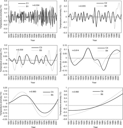
Fig. 2 The global mean temperature, which was simulated by the BCC-CSM1-1 (BCC) model, its EEMD-improved simulations (BCC minus EEMD), its WTM-improved simulations (BCC minus WTM) and the observation (CRU) from 1901 to 2005.

3.2. Application in the simulation of every model

3.2.1. Global scale.

Global average annual temperature simulated by eight AOGCMs between 1901 and 2005 were decomposed using EEMD. The statistics (correlation, bias, and RMSE) between model simulations and CRU were calculated to investigate the improvement of model simulations by EEMD (Fig. 3). The correlation coefficient increased after being filtered by EEMD for every model. The increment in correlation was more obvious for the CNRM, CAN, GISSH, and NOR models. The correlation coefficients increased over 0.03 for most models (Table 2). The percentage improvement in correlation was greater than or equal to 5% for CAN (7%), CNRM (12%), GISSH (5%), IPSL (5%), and NOR (9%). Bias and RMSE, which indicated the distance and error between model simulations and the observation, were reduced after they were filtered by EEMD for every model (Fig. 3). After being filtered by EEMD, the decrease in the percentage of bias and RMSE was almost 5% for each model and the percentage decrements were greater than 15% for some models (Table 2).

Fig. 3 Correlation, bias and RMSE of the original model simulations, EEMD-improved series and WTM-improved series for every model at the global scale.

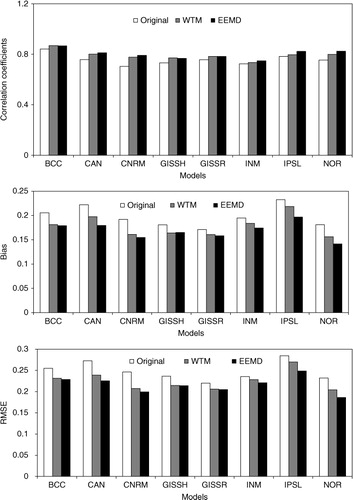
Table 2. Statistics (correlation, bias, RMSE) between EEMD-improved model series and original model series (E minus O) and its percentage variation [calculated by (E−O)/O×100]

Correlation		Bias		RMSE
E minus O	%	E minus O	%	E minus O	%
BCC	0.02	3	0.03	13	0.03	10
CAN	0.06	7	0.04	19	0.05	17
CNRM	0.09	12	0.04	19	0.05	19
GISSH	0.04	5	0.02	9	0.02	9
GISSR	0.03	3	0.01	7	0.02	7
INM	0.02	3	0.02	11	0.01	6
IPSL	0.04	5	0.04	16	0.04	13
NOR	0.07	9	0.04	22	0.05	20

After the model simulations were filtered by WTM (Fig. 3), the increase in correlation coefficient and decrease in both bias and RMSE showed that the model performances could be improved using WTM. However, the increase in correlation and decrease in bias and RMSE were less when using WTM as opposed to EEMD. Thus, WTM was less effective than EEMD in improving the model performances on the global scale.

3.2.2. Continental scale.

The improvement in model performance was also checked on the regional scale. The global land area was divided into six continents except Antarctica. Regional average temperatures were calculated for each continent between 1901 and 2005. The regional temperature series was decomposed using EEMD and WTM for every model. The statistics (correlation, bias, and RMSE) between model simulations and CRU data were calculated to test the model performance on the continental scale (Fig. 4). Increased correlation was found in every continent for different models when the EEMD mode elimination method was used. The improvements in correlation were especially obvious in Africa, Asia and Europe. In each continent, the percentage increment in correlation was greater than 15% in some models. The bias and RMSE decreased in the EEMD-improved series (Fig. 4). The reduction in bias and RMSE were low in Africa and Asia. A significant decrease in bias was found in Australia and Europe. The percentage decrements were greater than 10% for some models in Australia and Europe. The decrease of RMSE was more obvious in Australia, Europe, and North America. In these continents, the percentage decrease in RMSE was greater than 5% for most models. Overall, the bias and RMSE decreased more in Australia, Europe and North America than in the other continents.

Fig. 4 Correlation, bias and RMSE of original model simulations, EEMD-improved series and WTM-improved series for every model in the six continents.

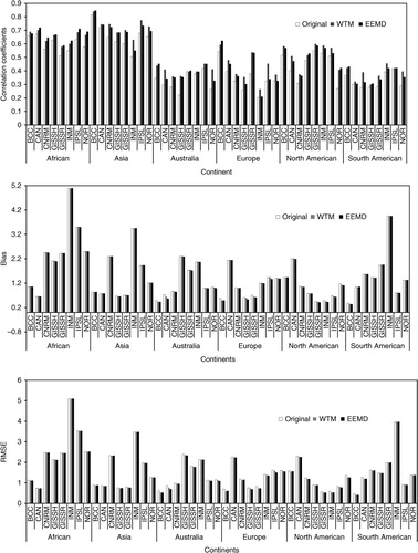
An increase in correlation was found in every continent for different models when WTM was used (Fig. 4). However, the bias and RMSE changed little when WTM was used. Moreover, the increase in correlation and decrease in bias and RMSE were less when WTM was used than when EEMD was used in most continents for most models. Thus, WTM was not as effective as EEMD in improving the model simulations on the continental scale.

3.3. Application of improved model simulations in MMEs

3.3.1. Improvement of MMEs calculated based on the improved model simulations on the global scale.

Because EEMD was more efficient than WTM with regards to improving model performances, the EEMD-improved model simulations were used to calculate the MME simulations based on four MME methods (AEM, Linear, SVD, and Bayesian). The MME simulations, which were calculated using EEMD-improved model simulations, were compared with those calculated using the original model simulations to investigate the improvement in MME simulations. The statistical parameters (correlation, bias, and RMSE) were calculated for MME simulations using EEMD-improved model simulations and original model simulations (Fig. 5). The MME simulations based on EEMD-improved model simulations were more closely correlated than the MME simulations based on the original simulations. The correlation coefficients increased by approximately 0.01–0.02 when EEMD-improved simulations were used (Table 3). The percentage increment in correlation was between 1 and 2.5%. The bias and RMSE of the ensembles based on EEMD-improved simulations were lower than the ensembles based on the original simulations. The percentage decrements in bias and RMSE were between 4 and 6% (Table 3).

Fig. 5 The statistics (correlation, bias, and RMSE) of MME forecasts calculated by the four MME methods (Bayesian, Linear, SVD, and AEM) based on the original and EEMD-improved model simulations at the global scale.

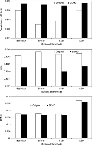
Table 3. Differences between the statistics (correlation, bias, RMSE) between ensemble forecasts based on EEMD-improved model series and original model series (E minus O) and the percentage differences [calculated by (E−O)/O×100]

Statistics	E minus O	Percentage difference
Correlation	Bayesian	0.009	1.094
Linear	0.017	2.000
SVD	0.021	2.481
AEM	0.009	1.094
Bias	Bayesian	−0.006	4.316
Linear	−0.010	6.844
SVD	−0.009	6.769
AEM	−0.006	4.644
RMSE	Bayesian	−0.006	3.501
Linear	−0.009	4.823
SVD	−0.011	6.122
AEM	−0.010	3.606

3.3.2. Improvement of MMEs on the continental scale.

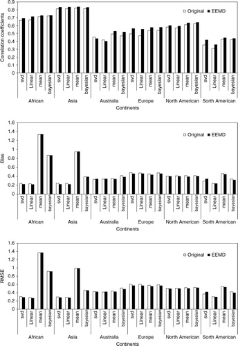
On the continental scale, the improvement in MME results was also investigated by comparing the MME simulation calculated using the EEMD-improved model simulations with those calculated based on the original model simulations. The statistical correlation between the MME simulations and observations is shown in Fig. 6. The ensemble results based on the EEMD-improved series had better correlation than the ensemble results based on the original series. The maximum increase in the correlation coefficient was greater than 0.2, with an increase of greater than 0.05 for many continents. For some continents, the percentage increment in correlation was greater than 10%. For EEMD-improved simulations, the increase in correlation was more obvious in Europe, South America, and North America. The bias and RMSE of ensemble forecasts were reduced when they were calculated based on the EEMD-improved simulations (Fig. 6). The bias and RMSE decreased by in excess of 0.04 and the percentage decrement was greater than 5% in many continents for the EEMD-improved simulations. Overall, the MME simulations could be further improved when calculated using the EEMD-improved temperature simulations on the continental scale.

Fig. 6 The statistics (correlation, bias, RMSE) of MME simulations calculated by the four MME methods (Bayesian, Linear, SVD, AEM) based on the original and EEMD-improved model simulations in six continents.

3.4. Application to future scenarios exemplified by global mean temperature

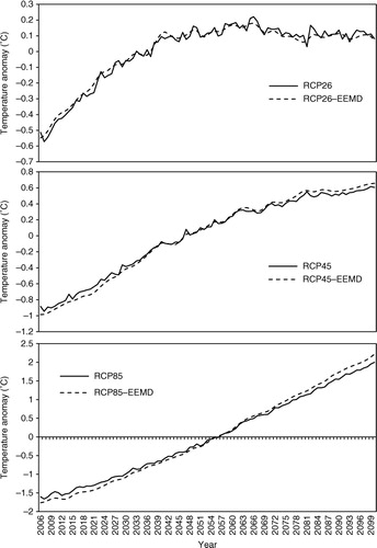
Future global mean temperatures were simulated from 2006 to 2100 by AOGCMs under different forcing scenarios. The anomalies of these simulations were calculated and improved with the EEMD mode elimination method (Fig. 7). The ensemble mean temperature under scenario RCP (Representative Concentration Pathways) 2.6 showed a similar trend of increase as its EEMD-improved series. However, the ensemble mean temperatures under RCP4.5 and RCP8.5 showed lower trends of increase than their EEMD-improved series. Thus, the increasing temperature trend was slightly underestimated.

Fig. 7 Multi-model ensemble mean simulations of global annual mean temperatures for future scenarios (RCP2.6, RCP4.5 and RCP8.5) and their EEMD-improved series (RCP26 minus EEMD, RCP45 minus EEMD and RCP85 minus EEMD).

4. Discussion

A new method based on EEMD was developed to improve the temperature simulations of AOGCMs. EEMD, which can decompose time series into different frequency signals, was used to decompose the AOGCM temperature simulations. The signal could be decomposed into its intrinsic modes of oscillation by EEMD. The numbers of IMFs were certain when data were provided, as the EEMD is a data-driven, adaptive data method. The model simulations were adaptively decomposed into six IMFs by EEMD. The model simulations contained a climate change signal and inter-annual variations. Most signals contained in IMF1 were inter-annual signals. On the one hand, the IMFs of the model simulation were highly correlated with the corresponding IMFs of the observation, except IMF1; while on the other hand, GCMs were less effective in simulating the temperature below the inter-annual time scale. Thus, large differences between the original model simulation and the observation were reduced by removal of IMF1. The model simulation was more approximate to the observation after IMF1 was removed from the original model simulation.

In order to compare the EEMD method with the other filter method, the results of WTM were also presented. However, WTM was found to be less effective than EEMD in improving the model performances in this study. Thus, the simulated annual temperatures were improved by EEMD on global and continental scales. The correlations increased by 5% for most models on the global scale. The bias and RMSE decreased significantly with the increase in correlation. This suggests that the model performance was improved by the EEMD mode elimination method when applied to these models. The improvement of model performance was also shown on the continental scale. Almost all model results were poor on the continental scale when compared to the global-scale results. However, the improvement of model performance was larger on the continental scale than on the global scale, especially for the models that had low correlation coefficients in some continents. Overall, the EEMD mode elimination methods improved the model performance on global and continental scales for all models.

MME simulations were calculated based on the EEMD-improved simulations by the AEM, Linear, SVD and Bayesian methods. An improvement in MME simulations was found on both the global and continental scales. The MME methods gave weights to different models. Thus, it is not surprising that the MME simulations were improved when the simulation of each model was improved. The correlation coefficient increased by between 0.01 and 0.02 only on the global scale. This is probably because the correlation coefficients were high enough already (r>0.83) and were therefore difficult to improve. The correlation improvements of existing MME methods (Peng et al., 2002; Pagowski et al., 2005; Min and Hense, 2006) were also marginal when compared with the model that yielded the best performance value. Despite this, the improvement in correlation still accounted for 1–2% variation of the original correlation coefficients. Although the correlation coefficients changed only slightly, there was an obvious decrease in bias and RMSE. This suggests that the MME simulations were improved on the global scale. Moreover, the improvements in correlation were more significant on the continental scale than the global scale. The percentage increments in correlation were greater than 5% in many continents. Therefore, the correlation improved more readily on the continental scale than on the global scale. There was an obvious decrease in bias and RMSE on the continental scale when based on the EEMD-improved simulations. The decrease in bias and RMSE, with the increase in correlation, indicated a substantial improvement of the MME simulations on the continental scale. Overall, the results of the MME simulations were further improved by application of the EEMD mode elimination method on both the global and continental scales. However, it should be stated that the method was only used in temperature simulations by each model; the improvement in precipitation simulations will be reported in future work.

5. Acknowledgements

This work was funded by National Key Scientific Projects (2010CB950903 and 2012CB95570002) and the National Natural Science Foundation of China (41271066 and 31100327). We thank the two anonymous reviewers for their constructive comments. We acknowledge the World Climate Research Program's Working Group on Coupled Modelling, which is responsible for CMIP, and we thank the climate modelling groups for producing and making available their model output.

References

- Annan J. D. , Hargreaves J. C . Reliability of the CMIP3 ensemble. Geophys. Res. Lett. 2010; 37: L2703.
- Berliner L. M. , Kim Y . Bayesian design and analysis for superensemble-based climate forecasting. J. Clim. 2008; 21: 1891–1910.
- Breaker L. C. , Ruzmaikin A . The 154-year record of sea level at San Francisco: extracting the long-term trend, recent changes, and other tidbits. Clim. Dynam. 2011; 36: 545–559.
- Chen D. , Achberger C. , Räisänen J. , Hellström C . Using statistical downscaling to quantify the GCM-related uncertainty in regional climate change scenarios: a case study of Swedish precipitation. Adv. Atmos. Sci. 2006; 23: 54–60.
- Collins M. , Booth B. B. , Bhaskaran B. , Harris G. R. , Murphy J. M. , co-authors . Climate model errors, feedbacks and forcings: a comparison of perturbed physics and multi-model ensembles. Clim. Dynam. 2011; 36: 1737–1766.
- Daubechies I . Orthonormal bases of compactly supported wavelets. Commun. Pure Appl. Math. 1988; 41: 909–996.
- Daubechies I . Symmetry for Compactly Supported Wavelet Bases. Ten lectures on wavelets. 1992; Philadelphia: Society for Industrial and Applied Mathematics. 251–287.
- Doblas Reyes F. J. , Hagedorn R. , Palmer T. N . The rationale behind the success of multi-model ensembles in seasonal forecasting–II. Calibration and combination. Tellus A. 2005; 57: 234–252.
- Duan Q. , Ajami N. K. , Gao X. , Sorooshian S . Multi-model ensemble hydrologic prediction using Bayesian model averaging. Adv Water Resour. 2007; 30: 1371–1386.
- Feddersen H. , Navarra A. , Ward M. N . Reduction of model systematic error by statistical correction for dynamical seasonal predictions. J Clim. 1999; 12: 1974–1989.
- Franzke C . Long-range dependence and climate noise characteristics of Antarctic temperature data. J. Clim. 2010; 23: 6074–6081.
- Gates W. L. , Boyle J. S. , Covey C. , Dease C. G. , Doutriaux C. M. , co-authors . An overview of the results of the Atmospheric Model Intercomparison Project (AMIP I). Bull. Am. Meteorol. Soc. 1999; 80: 29–55.
- Giorgi F. , Mearns L. O . Calculation of average, uncertainty range, and reliability of regional climate changes from AOGCM simulations via the “reliability ensemble averaging” (REA) method. J. Clim. 2002; 15: 1141–1158.
- Giorgi F. , Mearns L. O . Probability of regional climate change based on the reliability ensemble averaging (REA) method. Geophys. Res. Lett. 2003; 30: 1629.
- Graps A . An introduction to wavelets. Comput. Sci. Eng. 1995; 2: 50–61.
- Hagedorn R. , Doblas Reyes F. J. , Palmer T. N . The rationale behind the success of multi-model ensembles in seasonal forecasting–I. Basic concept. Tellus A. 2005; 57: 219–233.
- Huang N. E. , Shen Z. , Long S. R . A new view of nonlinear water waves: the Hilbert spectrum 1. Annu. Rev. Fluid. Mech. 1999; 31: 417–457.
- Huang N. E. , Shen Z. , Long S. R. , Wu M. C. , Shih H. H. , co-authors . The empirical mode decomposition and the Hilbert spectrum for nonlinear and non-stationary time series analysis. Proc. Roy. Soc. Lond. 1998; 454: 903–995.
- Huang N. E. , Wu Z . A review on Hilbert-Huang transform: method and its applications to geophysical studies. Rev. Geophys. 2008; 46: G2006.
- IPCC (Intergovernmental Panel on Climate Change). Climate Change 2007: Synthesis Report. 2007; Cambridge: Cambridge University Press.
- Kharin V. V. , Zwiers F. W . Climate predictions with multimodel ensembles. J. Clim. 2002; 15: 793–799.
- Krishnamurti T. N. , Kishtawal C. M. , LaRow T. E. , Bachiochi D. R. , Zhang Z. , co-authors . Improved weather and seasonal climate forecasts from multimodel superensemble. Science. 1999; 285: 1548–1550.
- Krishnamurti T. N. , Kishtawal C. M. , Shin D. W. , Williford C. E . Improving tropical precipitation forecasts from a multianalysis superensemble. J. Clim. 2000; 13: 4217–4227.
- Min S. K. , Hense A . A Bayesian approach to climate model evaluation and multi-model averaging with an application to global mean surface temperatures from IPCC AR4 coupled climate models. Geophys. Res. Lett. 2006a; 33: L8708.
- Min S. K. , Hense A . A Bayesian assessment of climate change using multimodel ensembles. Part I: global mean surface temperature. J. Clim. 2006b; 19: 3237–3256.
- Pagowski M. , Grell G. A. , McKeen S. A. , Dévényi D. , Wilczak J. M. , co-authors . A simple method to improve ensemble-based ozone forecasts. Geophys. Res. Lett. 2005; 32: L7814.
- Peng P. , Kumar A. , van den Dool H. , Barnston A. G . An analysis of multi-model ensemble predictions for seasonal climate anomalies. J. Geophy. Res. 2002; 107: ACL–18.
- Qian C. , Fu C. , Wu Z. , Yan Z . On the secular change of spring onset at Stockholm. Geophys. Res. Lett. 2009; 36: L12706.
- Raftery A. E. , Gneiting T. , Balabdaoui F. , Polakowski M . Using Bayesian model averaging to calibrate forecast ensembles. Mon. Weather Rev. 2005; 133: 1155–1174.
- Reifen C. , Toumi R . Climate projections: past performance no guarantee of future skill. Geophys. Res. Lett. 2009; 36: L13704.
- Semenov M. A. , Stratonovitch P . Use of multi-model ensembles from global climate models for assessment of climate change impacts. Clim. Res. 2010; 41: 1–14.
- Shin D. W. , Krishnamurti T. N . Short-to medium-range superensemble precipitation forecasts using satellite products: 2. Probabilistic forecasting. J. Geophys. Res. 2003; 108: 8384.
- Tebaldi C. , Knutti R . The use of the multi-model ensemble in probabilistic climate projections. Phil Trans Roy. Soc A. 2007; 365: 2053–2075.
- Weigel A. P. , Liniger M. A. , Appenzeller C . Can multi-model combination really enhance the prediction skill of probabilistic ensemble forecasts?. Q. J. Roy. Meteorol. Soc. 2008; 134: 241–260.
- Weisheimer A. , Doblas-Reyes F. J. , Palmer T. N. , Alessandri A. , Arribas A. , co-authors . ENSEMBLES: a new multi-model ensemble for seasonal-to-annual predictions: Skill and progress beyond DEMETER in forecasting tropical Pacific SSTs. Geophys. Res. Lett. 2009; 36: L21711.
- Weisheimer A. , Smith L. A. , Judd K . A new view of seasonal forecast skill: bounding boxes from the DEMETER ensemble forecasts. Tellus A. 2005; 57: 265–279.
- Wu Z. , Huang N. E . Ensemble empirical mode decomposition: a noise-assisted data analysis method. Adv. Adapt. Data Anal. 2009; 1: 1–41.
- Wu Z. , Huang N. E. , Long S. R. , Peng C . On the trend, detrending, and variability of nonlinear and nonstationary time series. Proc Natl Acad Sci. 2007; 104: 14889–14894.
- Wu Z. , Schneider E. K. , Kirtman B. P. , Sarachik E. S. , Huang N. E. , co-authors . The modulated annual cycle: an alternative reference frame for climate anomalies. Clim. Dynam. 2008; 31: 823–841.
- Yun W. T. , Stefanova L. , Krishnamurti T. N . Improvement of the multimodel superensemble technique for seasonal forecasts. J. Clim. 2003; 16: 3834–3840.