
Abstract
This paper studies the question how the zonal mean potential vorticity (PV) distribution in potential temperature (θ) coordinates is established in the atmosphere by the interaction of diabatic processes (cross-isentropic transport of mass) with adiabatic dynamical processes (isentropic transport of mass and potential vorticity substance). As an aid in dissecting this interaction, a simplified model of the general circulation is constructed, which contains parametrisations of radiative transfer, wave drag and water cycle. This model reproduces the following four observed features of the atmosphere below 10 hPa: (1) a permanently present eastward subtropical jet, which in winter is separated from an eastward stratospheric jet by a zone (referred to as the ‘surf zone’), between θ=380 K and θ=550 K, where planetary wave drag reduces PV over the polar cap; (2) a stratospheric zonal wind reversal in spring or beginning of summer; (3) a tropical cold layer at 100 hPa, and (4) a realistic distribution of zonal mean cross-isentropic flow. The strength of the cross-isentropic flow depends on wave drag, latent heat release and the thermal inertia of both the atmosphere and the earth's surface. Of special interest is the layer between θ=315 K and θ=370 K (the ‘Middleworld’), which lies in the troposphere in the tropics and in the stratosphere in the extratropics. Mass converges diabatically into this layer in the deep tropics, mainly due to latent heat release, and diverges out of this layer elsewhere due to radiation flux divergence. Meridional isentropic vorticity flux divergence in the tropical Middleworld, associated with the upper branch of the Hadley circulation, creates a region in the subtropics, at θ=350 K and adjacent isentropic levels, with a marked isentropic meridional PV-gradient, forming the isentropic dynamical tropopause.
To access the supplementary material to this article, please see Supplementary files under Article Tools online.
1. Introduction
The interaction of adiabatic fluid dynamical processes with diabatic processes in the atmosphere is a fundamental problem of meteorology and has received incidental explicit attention principally as part of General Circulation Model (GCM) studies, which began at Princeton University more than 50 yr ago (Manabe et al., Citation1965; Smagorinsky et al., Citation1965; Manabe and Hunt, Citation1968). Although this interaction is incorporated into GCM's, this explicit attention has been limited until now to ‘radiative–dynamical’ interaction (e.g. Fels, Citation1985). Here we also study the interaction of the water cycle (latent heat release) with dynamics and radiation, hence the phrase, ‘diabatic–dynamical interaction’, to indicate this more comprehensive interaction. The aim of this paper is to disentwine the diabatic–dynamical interactions that establish the zonal mean global distribution of potential vorticity (PV) (defined in section 2) in the upper troposphere and lower stratosphere (UTLS).
This study is motivated by a previous paper (van Delden and Hinssen, Citation2012), in which it was demonstrated, by piecewise PV inversion, that the zonal mean subtropical jet and the zonal mean polar winter stratospheric jet are induced by well-defined anomalies in the zonal mean PV-distribution on isentropic surfaces. Identification of the physical mechanisms that lead to the formation of these PV-anomalies might represent an advance in our understanding of the zonal mean general circulation. It might also help to understand and predict the dynamical response of the atmosphere to changes in its composition (Fels et al., Citation1980; Hinssen et al., Citation2011b).
To the author's knowledge, previous research on the topic of the PV-budget and the question how the PV-distribution is established in the general circulation is very limited. The most important contributions in this respect were due to Hoerling (Citation1992), Koshyk and McFarlane (Citation1996) and Edouard et al. (Citation1997). These studies were however limited to either the analysis of the PV-budget of a specific simulation with a GCM or the analysis of the PV-budget of analyses of observations, which were assimilated with a numerical weather prediction model.
This paper focuses on illuminating the connection between the zonal mean PV-distribution and the following five interconnected features of the general circulation: (1) the subtropical tropospheric jets, (2) the tropical cold layer at 100 hPa, (3) the polar winter stratospheric vortex, (4) the stratospheric zonal wind reversal in spring and (5) the strong meridional slope of the dynamical tropopause in the subtropics. Smagorinsky et al. (Citation1965) were the first to produce a reasonably successful GCM-simulation of the tropical cold layer. A later version of this model with a higher vertical resolution produced separate jets in the subtropical upper troposphere and in the polar winter stratosphere (Manabe and Hunt, Citation1968). The first explicit and relatively successful simulation of the seasonal cycle of the zonal wind in the stratosphere, including seasonal zonal wind reversals, was due to Manabe and Mahlman (Citation1976). Subsequent studies, using GCMs with higher resolution, especially in the stratosphere, have quantitatively improved these results (Strauss and Shukla, Citation1988; Pawson et al., Citation2000). However, an explicit investigation, using a GCM, aimed at a systematic unravelling of the interactions between different diabatic and adiabatic processes that contribute to establishing the observed zonal mean PV distribution, has never been published before, probably because of the large complexity of GCMs, and maybe also because knowledge of a wide range of topics (dynamics, radiation, water cycle) is required to study this problem.
Here we take a step back to the basics. In the spirit of Ockham's razor and following the advice embodied in the last sentence of Smagorinsky (Citation1964), a highly simplified, but still rather complex, version of a GCM is constructed. This GCM reproduces the five features of the general circulation that are enumerated in the previous paragraph. A comparison of the dependence of the solutions of this model on the inclusion or exclusion, of ‘adiabatic dynamics’, of heat sources and sinks associated with evaporation and condensation of water, of absorption of solar radiation by ozone and water vapour and of planetary wave drag, yields insight into how these processes interact with emission and absorption of radiation by the earth's surface and by the atmosphere to produce the observed zonal mean PV distribution.
Section 2 describes the theoretical and observational background of this paper. Section 3 starts by studying the relatively simple problem of an idealised atmosphere, containing only one well-mixed absorber and emitter of long wave radiation, like carbon dioxide, which is in exact radiative equilibrium and hence devoid of cross-isentropic flow. With the assumption that the well-mixed greenhouse gas absorbs long wave radiation as a grey absorber, the radiative equilibrium temperature is evaluated analytically.
Because both the atmosphere and the earth's surface have a finite heat capacity, radiative equilibrium is in reality not attained anywhere at any point in time. Taking these heat capacities into account results in the ‘radiatively determined’ state. For the same idealised atmosphere, the ‘radiatively determined’ state is more realistic than the radiative equilibrium state, but still has deficiencies, obviously due to the neglect of the circulation. The interaction between circulation and radiation is studied with the aforementioned GCM, which is described in section 4. The results of permanent equinox model integrations, without a water cycle, are discussed in section 5. In section 6, an energy conserving representation of the water cycle is added to the model. Cooling of the earth's surface due to evaporation of surface water and heating of the atmosphere above cloud base, due to latent heat release, especially in the tropics, are taken into account. The permanent equinox simulation of the zonal mean circulation, including the water cycle, produces a realistic subtropical jet, as well as tropical cold layer at approximately 100 hPa.
In section 7, the PV-budget equation, introduced in section 2, is used to provide insight into the most important physical mechanisms that establish the PV-distribution in the simplified model. In section 8, a seasonal cycle is introduced by assuming a realistic obliquity of earth's axis and prescribing the observed seasonal cycle of ozone concentrations. The paper is concluded in section 9.
2. Theoretical and observational background
Potential vorticity in the isentropic coordinate system is defined as1
where ζ
θ
is the relative vorticity on an isentropic surface (constant potential temperature, θ), f is the planetary vorticity, or Coriolis parameter, and σ is the hydrostatic isentropic density, which is defined in terms of pressure, p, and θ as2
where g is the acceleration due to gravity (Holton, Citation2004).
Following Hinssen et al. (Citation2010), PV in the zonal mean reference state is defined as,3
where reference isentropic density is4
The integral is over latitude, φ, from 10°N to 90°N or from 10°S to 90°S, while the square brackets indicate a zonal mean. The reference isentropic density, corresponding to one hemisphere, is independent of latitude. Inversion of the reference PV-distribution, poleward of φ=±10°, assuming no thermal wind at the earth's surface and [u]=0 at the upper- and side-boundary, yields the state of rest with respect to the surface of the earth (van Delden and Hinssen, Citation2012). Hence zonal mean PV-anomalies and/or temperature anomalies at the earth's surface are responsible for inducing the zonal mean currents poleward of φ=±10° in an atmosphere that is in thermal wind balance. A PV-anomaly, Z′, is defined as5
Following Hoskins (Citation1991), the dynamical tropopause is defined as the ±2 PVU isopleth of PV (1 PVU=10−6 K m2 kg−1 s−1). The dynamical tropopause is indicated in by the thick green contour, labelled 2 PVU in the northern hemisphere and −2 PVU in the southern hemisphere. Due to the latitude-dependence of both f and σ, the dynamical tropopause slopes downward from the tropics toward the poles. The ‘reference dynamical tropopause’, on which Z ref=±2 PVU is indicated in by a thin green line. The relatively low value of σ between θ=315 K and θ=370 K in the extratropics has the effect of lowering the tropopause there, relative to reference tropopause. This is a manifestation of the presence of the so-called ‘ex-UTLS PV-anomaly’, which induces the zonal mean subtropical jet (van Delden and Hinssen, Citation2012). The acronym ‘ex-UTLS’ stands for ‘extratropical upper troposphere and lower stratosphere’ (Gettelman et al., Citation2011).
Fig. 1 January average zonal mean pressure (dotted black lines, labelled in units of hPa), potential vorticity (thick green lines, labelled in PVU), reference potential vorticity (thin green lines, labelled in PVU), cross-isentropic flow (labelled in units of K day−1; blue: downwelling; red: upwelling) and temperature (cyan; only the 200 K isotherm) as a function of latitude and potential temperature, according to the ERA-40 re-analysis (Uppala et al., Citation2005) and CIRA (Fleming et al., Citation1990). The thick black line indicates the zonal mean position of the earth’ surface. The black dashed–dotted lines indicate the top and bottom of the Middleworld. The ERA-40 average is for the period 1979–2002. ERA-40 data: provided by Paul Berrisford.
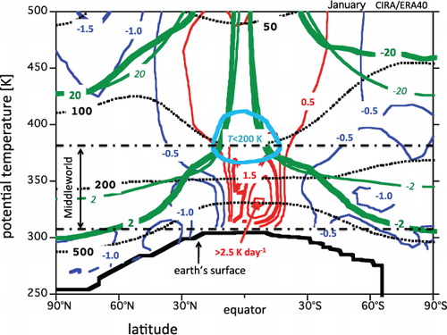
Approaching the equator, the dynamical tropopause loses its meaning. An appropriate definition of the tropical tropopause is the ‘cold point tropical tropopause’ (Highwood and Hoskins, Citation1998), which coincides with the tropical temperature minimum at about 100 hPa or θ=380 K ().
also shows the cross-isentropic flow, i.e. the quantity, , which represents the vertical branch of the ‘diabatic circulation’ (Holton, Citation2004). Although the magnitude of the cross-isentropic flow is uncertain (Fueglistaler et al., Citation2009), there is no doubt that, below θ=600 K, it is upward in the tropics and almost uniformly downward over the polar cap, even in the summer hemisphere. The intense ‘plume’ of upward cross-isentropic flow in the tropical troposphere is a reflection of latent heating, while the broad ‘plume’ of upward cross-isentropic flow in the tropical lower stratosphere is a reflection of the effect of planetary waves in driving the lower stratosphere out of radiative equilibrium.
Hoskins (Citation1991) introduced a very useful three-fold division of the atmosphere into the ‘Overworld’ (the region encompassed by isentropic surfaces that are everywhere above the tropopause), the ‘Middleworld’ (the region encompassed by isentropes that cross the dynamical tropopause and do not strike the earth's surface) and the ‘Underworld’ (the region encompassed by isentropic surfaces that intercept the earth's surface). Hoskins (Citation1991) noted that the zonal mean PV in the ‘Middleworld’ exhibits interesting features, such as the enhanced meridional PV-gradient in the subtropics ().
Because the maximum cross-isentropic upwelling is observed in the tropical lower Middleworld, near 315 K, the tropical Middleworld, which resides completely in the troposphere, is inflated with mass. In the tropics, the layer between θ=315 K and θ=370 K contains roughly 60% of the total mass of the tropical atmosphere per unit horizontal area. In the extratropics, poleward of 50°, this Middleworld layer resides in the stratosphere and represents less than 25% of the total mass of the atmosphere per unit horizontal area. The associated meridional isentropic density gradient in the Middleworld is revealed in by the opposing slopes of isobars in the subtropics above and below θ=350 K. This feature of the zonal mean mass distribution can be understood from the equation of mass conservation in isentropic coordinates:6
Here, , while the isentropic density flux,
, is defined as
7
where u and v are the x- and y-component of the velocity.
The diabatic (cross-isentropic) component of the net isentropic density flux, denoted by I
d
, into a layer bounded by two isentropic surfaces, labelled ‘1’ and ‘2’, where level 1 represents the lower boundary and level 2 represents the upper boundary, is evaluated from the following expression:8
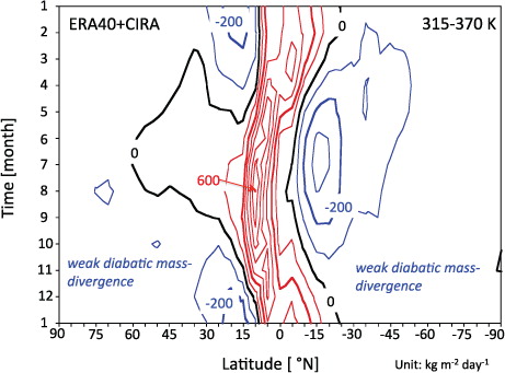
Isentropic density is determined to first order by radiation. The ‘radiatively determined’ isentropic density decreases with increasing height from a value in the order of 1000 kg m−2 K−1 at θ=315 K to a value in the order of 10 kg m−2 K−1 at θ=370 K ( of van Delden and Hinssen, Citation2012), so that in this layer σ 1 is much larger than σ 2.This implies that, if θ 1≈θ 2, an upward diabatic mass flux (in the tropics) is associated with I d >0, whereas a downward diabatic mass flux (in the extratropics) is associated with I d <0. This is confirmed in , which indicates that I d in the layer between 315 K (level 1) and 370 K (level 2) is indeed positive in the deep tropics and negative in the subtropics and extra-tropics. The largest negative values are observed in the subtropical winter hemisphere, in connection with the downward branch of the winter Hadley cell. The upward branch of the Hadley circulation is revealed in as a narrow region with a large positive net diabatic mass flux. This region is known as the Inter-Tropical Convergence Zone (ITCZ). During the northern hemisphere monsoon up to 600 kg m−2 day−1 converges into the Middleworld in the ITCZ, implying that the total mass in this layer is replenished approximately every 10 d. Note that the zonal mean meridional width of the ITCZ is about 2000 km. The maximum excursion from the equator of the zonal average ITCZ is about 10°.
Fig. 2 Average yearly cycle of the diabatic convergence of mass per unit area into the Middleworld layer between θ=315 K and θ=370 K. Labels indicate diabatic mass flux convergence in units of kg m−2 day−1. The figure is based on the ECMWF ERA-40 re-analysis of the monthly mean zonal mean diabatic heating and the monthly mean isentropic density at θ=315 K and at θ=370 K, according to the CIRA (Fleming et al., Citation1990).
PV is sometimes interpreted as being the mixing ratio of a conserved quantity called ‘potential vorticity substance’, PVS (=σZ) (Haynes and McIntyre, Citation1987, Citation1990). Local changes of PVS are determined by the following equation, which is very similar to eq. (6).9
The flux of PVS is10
Here, F x and F y are frictional forces per unit mass. The flux of PVS has no component across isentropic surfaces. This means that isentropic surfaces are impermeable to PVS [eq. (10)], but permeable to mass [eq. (7)]. Hence cross-isentropic flow may lead to dilution or to concentration of PVS, and so lead to the appearance of PV-anomalies.
The local PV-budget can be understood from the equation governing the local time tendency of PV [the combination of eqs. (6) and (9)]:11
This equation reveals how both mass flux divergence and isentropic PVS flux divergence determine the local PV-budget.
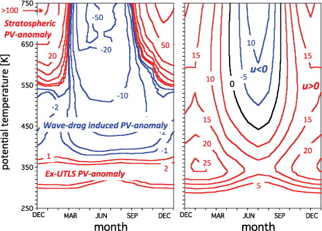
(left panel) shows the amplitude of the average PV-anomaly over the North Polar cap (north of 65°N) as a function of time and θ. A positive PV-anomaly (the polar part of the ex-UTLS PV-anomaly) at these high latitudes is present permanently between θ=310 K and θ=370 K. A negative PV-anomaly is observed between θ≈380 K and θ≈550 K. This PV-anomaly is a manifestation of the ‘surf-zone’ (McIntyre and Palmer, Citation1984). Above θ≈550 K the PV-anomaly is positive in winter and negative in summer. A positive PV-anomaly induces a cyclonic polar vortex (zonal mean zonal wind, [u]>0). The negative PV-anomaly in summer, which is observed at all levels above θ≈380 K, induces the anticyclonic polar summer vortex (zonal mean zonal wind, [u]<0) (van Delden and Hinssen, Citation2012). The reversal of the sign of the stratospheric PV-anomaly above θ=550 K in March or April from positive to negative is accompanied by a reversal of the zonal mean zonal wind from eastward to westward above θ=450 K. This wind reversal, however, may in some years occur in May, as can be seen in of Hinssen et al. (2011a).
Fig. 3 Left panel: yearly cycle of the area-weighted amplitude of the monthly mean PV-anomaly north of 65°N, as a function of time and potential temperature. Red contours: positive anomaly; blue contours: negative anomaly. Labels are in units of PVU. The ±1, ±2, ±5, ±10, ±20, ±50 and ±100 PVU contours are drawn. Right panel: yearly cycle of the area-weighted zonal wind between 30°N and 60°N. Contour interval is 5 m s−1. Labels are indicated in units of m s−1. Based on the CIRA (Fleming et al., Citation1990).
3. Radiative equilibrium state and ‘radiatively determined’ state
Throughout this paper, the plane-parallel assumption is adopted for radiative transfer calculations, i.e. the atmosphere is divided into air columns, which act independently as far as transfer of radiation is concerned. In this section, the atmosphere is assumed to be transparent to solar radiation and to contain one well-mixed greenhouse gas. This greenhouse gas absorbs long wave radiation as a grey absorber. The earth's surface absorbs 70% of the solar irradiance and absorbs and emits long wave radiation as a black body. The radiative equilibrium potential temperature in this atmosphere is (Pierrehumbert, Citation2010, section 4.3.4)12
Here, Q is the absorbed solar irradiance, p is pressure, p
ref
=1000 hPa, σ
B is the Stefan–Boltzmann constant, and κ=R/c
p
, where R and c
p
are, respectively, the specific gas constant of dry air and the specific heat capacity of air at constant pressure. The long wave optical path, δ, is defined as,13
Here σ m is the long wave absorption cross-section of the well-mixed greenhouse gas and q m is the constant specific concentration by mass of this gas. The specific concentration by volume of the well-mixed greenhouse gas is assumed to be 400 ppmv. In order to convert this number into a specific concentration by mass we must multiply it by the ratio of specific gas constants of dry air (R) and of the well-mixed greenhouse gas (R m ). If carbon dioxide is the well-mixed greenhouse gas, this ratio is R/R m =287/189. Furthermore, we assume that σ m =0.3 m2 kg−1. With these numbers, the optical path at the earth's surface (at p=105 Pa) is δ s =1.8.
The radiative equilibrium isentropic density, deduced from eqs. (2), (12) and (13), is14
This equation indicates that σ eq=0 at the top of the atmosphere (TOA), where p and δ are zero also. Furthermore, σ eq decreases with increasing Q.
The value of σ eq is positive everywhere in the atmosphere, i.e. the atmosphere in radiative equilibrium is statically stable. However, the radiative equilibrium temperature of earth's surface is higher than the radiative equilibrium temperature of the atmosphere just above. A little heat diffusion from the surface to the atmosphere would render the lower atmosphere statically unstable. It is important to note that we do not take this non-radiative effect into account in this section.
Let us neglect the daily cycle of Q, and assume a perfectly circular orbit of the earth around the sun, i.e. zero eccentricity and an obliquity of earth's axis of rotation equal to 23.45°. The absorbed solar radiation, Q, as a function of latitude and ordinal date can then easily be calculated (Pierrehumbert, Citation2010, section 7.3).
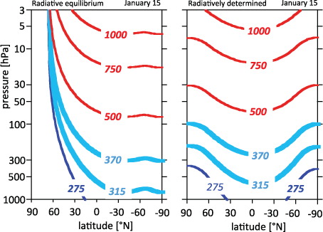
(left panel) shows the radiative equilibrium potential temperature, according to eq. (12), as a function of latitude and pressure on January 15, in an atmosphere with the properties given in the paragraphs above. As expected, the meridional temperature gradient in the summer hemisphere is practically zero. In the Polar night, the concept of radiative equilibrium is meaningless, except if we accept a radiative equilibrium temperature of absolute zero.
Fig. 4 Radiative equilibrium potential temperature (left panel) and radiative determined potential temperature (right panel), labelled in K, as a function of latitude and pressure on 15 January for an atmosphere which is transparent to solar radiation and contains one well-mixed greenhouse gas. The albedo of the earth's surface is 0.3. The result shown in the right panel is for C=5×10⁷ J K−1 m−2. The cyan contours represent isentropes in the Middleworld. The red contours represent isentropes in the Overworld. The dark blue contour is an isentrope in the Underworld. In the Polar night poleward of about 67°N, the radiative equilibrium temperature is absolute zero Kelvin (left panel).
Clearly, the assumption of radiative equilibrium is unrealistic. Because of the finite thermal inertia of the atmosphere and earth's surface, radiative equilibrium is never reached. A time lag of more than a month in the seasonal cycle of the temperature compared to the seasonal cycle of insolation is introduced due to the non-zero heat capacity of the atmosphere, which prevents very low Polar winter temperatures. Thermal inertia plays a very important role in determining both the temperature distribution and the cross-isentropic flow in earth's atmosphere.
The ‘radiatively determined’ state, which takes account of thermal inertia, is determined numerically by dividing the atmosphere into 200 layers of equal mass and formulating differential equations for the radiation budget of each layer and for the earth's surface. The radiation budget of the earth's surface is determined by the following time (t) dependent first order ordinary differential equation:15
Here, C is the heat capacity of the earth's surface (unit: J K−1 m−2), also called ‘thermal inertia coefficient’ by Pierrehumbert (Citation2010) (p. 445), T s is the temperature of the earth's surface, Q is the absorbed solar radiation and B is the long wave radiation received from the atmosphere, which is fully absorbed by the earth's surface. The radiation budget equation for an atmospheric layer is very similar. The thermal inertia coefficient of an atmospheric layer with a mass of Δp/g, where Δp is the pressure difference across the layer, is c p Δp/g.
The resulting 201 coupled ordinary differential equations are integrated numerically for several years, with identical external conditions (insolation as a function latitude and ordinal date) and internal conditions (composition of the atmosphere, surface pressure, value of the absorption cross-section). The right panel of shows the ‘radiatively determined’ potential temperature as a function of latitude and pressure for January 15, when C=5×10⁷ J K−1 m−2. This value corresponds to the heat capacity of a layer of water with a thickness of about 12.5 m. The total heat capacity of the atmosphere is c p p s /g≈107 J K−1 m−2. Therefore, in this example the thermal inertia of the system (earth's surface plus atmosphere) is determined principally by the thermal inertia of earth's surface.
In the ‘radiatively determined’ state, the summer pole does not become warmer than the tropics and the polar night atmosphere does not become colder than about –100°C. Therefore, the ‘radiatively determined’ state is much more realistic than the radiative equilibrium state. However, a striking difference between the ‘radiatively determined’ state and the observed state, which is shown in , is the absence in the ‘radiatively determined’ state of the tropical upward bulge of the 370 K isentrope, i.e. the tropical temperature minimum ().
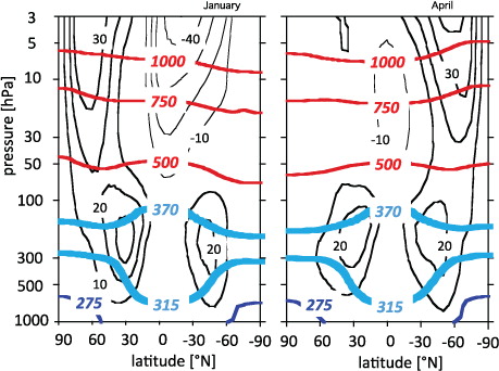
Fig. 5 Observed (CIRA: COSPAR International Reference Atmosphere) monthly average zonal average potential temperature, labelled in K (blue: Underworld; cyan: Middleworld; red: Overworld), and zonal mean zonal wind (black), labelled in m s−1, as a function of latitude and pressure for January (left panel) and for April (right panel).
shows the ‘radiatively determined’ cross-isentropic flow as a function of latitude and pressure on January 15 in year 4 for two values of the thermal inertia coefficient, C [eq. (15)]. Other conditions are identical in both cases. Clearly, the intensity of the cross-isentropic flow depends very strongly on the value of C. The ‘radiatively determined’ cross-isentropic flow is downward in the winter hemisphere and upward in the summer hemisphere during most of the year, except during a short period of transition around the equinoxes.
Fig. 6 ‘Radiatively determined’ cross-isentropic flow (labelled in units of K day−1; contour interval is 0.25 K day−1; zero contour not drawn) as a function of latitude and pressure for January 15 (in the fourth year), for two values of the thermal inertia coefficient, C: in the left panel C=106 J K−1 m−2; in the right panel C=5×10⁷ J K−1 m−2. The atmosphere is assumed to be transparent to solar radiation and contains one well-mixed greenhouse gas. The earth's surface albedo is 0.3 [see the text below eq. (13)].
![Fig. 6 ‘Radiatively determined’ cross-isentropic flow (labelled in units of K day−1; contour interval is 0.25 K day−1; zero contour not drawn) as a function of latitude and pressure for January 15 (in the fourth year), for two values of the thermal inertia coefficient, C: in the left panel C=106 J K−1 m−2; in the right panel C=5×10⁷ J K−1 m−2. The atmosphere is assumed to be transparent to solar radiation and contains one well-mixed greenhouse gas. The earth's surface albedo is 0.3 [see the text below eq. (13)].](/cms/asset/15da98a5-db78-4cff-ad57-10db16b72327/zela_a_11817037_f0006_ob.jpg)
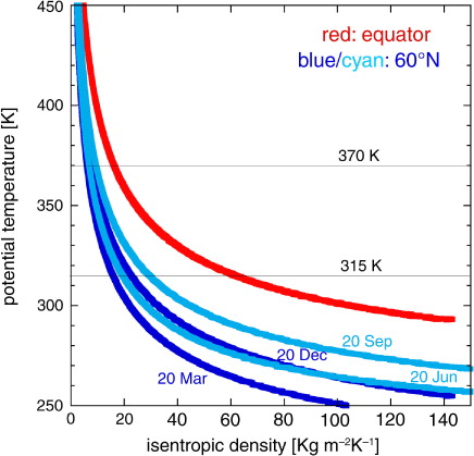
Because Q varies little in the tropics, cross-isentropic flow is practically non-existent at the equator, so that the ‘radiatively determined’ isentropic density, σ rad, hardly varies with the seasons here (). Indeed, σ rad≈σ eq at the equator. In the extra-tropics σ rad undergoes a marked seasonal cycle, with highest values at the end of summer and lowest values at the end of winter. According to the arguments given in section 2, this can be understood by observing that mass converges diabatically into existing isentropic layers in connection with radiative heating in summer, while mass diverges out of existing isentropic layers in connection with radiative cooling in winter. In the latter case, mass is stored in new isentropic layers in the lowest part of the Underworld, as was explained first by Shaw on page 329 of volume 4 of his Manual of Meteorology (Citation1931). Note that there is no flow along isentropes in the ‘radiatively determined’ atmosphere.
Fig. 7 ‘Radiatively determined’ isentropic density, σ rad, as function of potential temperature at the equator and at 60°N, for four different ordinal dates in year 3 of the integration of the radiation model for an atmosphere containing one well mixed greenhouse gas (see the text) and with C=5×10⁷ J K−1 m−2. The ordinal dates are 20 March, 20 June, 20 September and 20 December. The isentropic density profile at the equator is nearly identical for all four dates. The layer between 315 K and 370 K represents the Middleworld, which lies in the tropical troposphere and in the extratropical stratosphere.
In an atmosphere with a finite heat capacity, which contains one well mixed greenhouse gas, σ rad decreases from the equator to the pole at all times and at all heights (). This implies the existence of a ‘radiatively determined’ hemispheric wide permanent PV-anomaly, centred over the polar cap at all heights, which presumably induces one hemispheric-wide eastward zonal wind jet in both summer and winter. This is in contrast to reality (). In the following the dynamical response of the atmosphere to the radiatively imposed PV-distribution is studied by coupling the grey long wave radiation scheme of this section to a zonally symmetric hydrostatic primitive equation model, which includes parametrisations of dry convective adjustment and wave drag. In section 6, a simplified representation of the water cycle is added to this model.
4. A model of zonally symmetric radiative–dynamical adjustment
Zonal symmetry implies that the variables depend only on time, latitude and height. The effect of meridional transfer of momentum and heat by zonally asymmetric eddies on the zonal mean state is modelled by introducing a body force, or drag, D, in the zonal component of the equation of motion.
The model is hydrostatic and employs η=p/p
s
as a vertical coordinate, where p
s
is surface pressure. The symbol η is used here instead of the more conventional symbol, σ, because the latter symbol is used for isentropic density. Neglecting the terms, which are associated with the convergence of the meridians, the continuity equation is (Washington and Parkinson, Citation1986, chapter 3)16
Here, u and v are, respectively, the zonal (x-) and meridional (y-) components of the velocity. Other prognostic equations in this coordinate system (also neglecting the effect of the convergence of the meridians) are (Washington and Parkinson, Citation1986),17
18
19
20
Here, Φ is geopotential (=gz) and J is the diabatic heating rate per unit mass. The wave drag, D, is specified below. The terms F x and F y represent friction in the lower part of the atmosphere (see below). The term H represents vertical transport of heat due dry convective adjustment (see below). For simplicity, but ensuring kinetic energy conservation, all terms associated with earth's curvature have been neglected, except the ‘tan φ’ terms in eqs. (18) and (19).
Supplemented by the hydrostatic equation,21
these equations are solved numerically on a vertically staggered and horizontally non-staggered grid. The grid distance is 2° in φ and 0.005 in η, making a total of 91 grid points between the South Pole and the North Pole and 200 layers of equal mass. The simple vertical discretisation makes the coupling to the radiation scheme straightforward and accurate. Vertical velocity, dη/dt, is defined on the boundary of each layer. At the upper (η=0) and lower (η=1) boundary dη/dt=0. Horizontal velocity and temperature are defined at 200 intermediate points between η=0.0025 and η=0.9975. At the poles u=v=∂T/∂y=0. MacCormack's scheme (Mendez-Nunez and Caroll, Citation1993) is used to approximate the horizontal- and time derivatives in eqs. (16–19), while centred finite differences are used to approximate vertical derivatives. The Coriolis term is computed as an average over the gridpoints that are used to approximate the horizontal pressure gradient, consistent with MacCormack's scheme. The r.h.s. of eq. (20) is approximated by centred differences, while the time derivative on the left hand side of this equation is approximated as in the MacCormack's scheme. Velocity, temperature and surface pressure are smoothed with a five-point filter [eq. (32) of Shapiro, Citation1970] once every 12 hours.
Long wave radiative transfer is grey, as in section 3. The long wave optical path, δ, of a model layer (of thickness, dp) is determined by eq. (13), if the atmosphere is devoid of water, or eq. (31) (section 6), if the atmosphere contains water vapour.
As in section 3, the earth's surface is assumed to be a slab of matter with a fixed heat capacity C and with a constant albedo (=0.3). The potential temperature at the earth's surface is governed by an energy budget equation, as eq. (15), but with additional terms on the right hand side, representing fluxes of sensible heat and latent heat (see below).
Sensible heat transfer, H
s
, from the earth's surface to the atmosphere, due to static instability just above the surface (this effect was neglected in the calculation of the ‘radiatively determined’ state), is parametrised by the following equation:22
Here, θ s is the potential temperature of earth's surface, θ a is the potential temperature at the lowest atmospheric model level (η=0.9975) and the transfer coefficient, k H =50 W m−2 K−1. If the potential temperature within a particular layer in the interior of the atmosphere decreases with height, this parametrisation is also applied to this layer [the third term on the r.h.s. of eq. (17)].
In order to take account of absorption of solar radiation by ozone and water vapour, the solar spectrum is split into four bands. Each band represents a fixed proportion of the total solar irradiance (). Band 1 represents ultra-violet light, band 2 represents the wavelengths between the ultra-violet and the Chappuis band (band 3), and band 4 represents the near infrared. Ozone absorbs solar radiation in bands 1, 2 and 3. The values of the associated absorption cross-sections are listed in . Water vapour absorbs solar irradiance only in band 4 (section 6). The solar zenith angle is constant during one day and depends on the length of daylight. Ozone concentrations are prescribed according to an analysis of monthly mean, zonal mean observed ozone concentrations (Fortuin and Kelder, Citation1998).
Table 1. Absorption cross-sections of ozone (per molecule) and of water vapour (per kg) in the four solar spectral bands
The last term on the r.h.s. of both eq. (18) and eq. (19) represents friction in the turbulent boundary layer. Following the paper by Held and Suarez (Citation1994), it is assumed that this effect is relaxational, i.e. the frictional force is proportional to the velocity as follows:23
Here,24
with k f =10−4 s−1 and η b =0.7. This implies that the strongest effect of this ‘Rayleigh friction’ is confined to the layer below η=0.7.
The term D in eq. (18) represents planetary wave drag. This negative (westward) extra-tropical zonal force is associated with meridional isentropic transport and mixing of PV by planetary waves, which modifies the induced zonal mean balanced zonal flow (Hartmann, Citation2007). As was advocated by Haynes et al. (Citation1996), this force is treated entirely separately from boundary layer friction. Following the work by Plumb and Eluszkiewicz (Citation1999), this term is parametrised as follows:25
where26
and27
28
The parameter, D 0, is a specified constant with D 0=0, if u<0 at any lower level in the atmosphere, and D 0<0, if u≥0 at all lower levels. A reasonable assumption is D 0=−5×10⁻⁵ m s−2 if u≥0 at all lower levels. This parametrisation is based on a theory, which states that planetary waves do not propagate upward through a region with westward winds (Charney and Drazin, Citation1961). This means that planetary wave drag is non-existent at all levels above a layer with westward winds.
Others have adopted similar parametrisations of wave drag in simplified two-dimensional models of the atmospheric general circulation, with variations in the chosen values of D 0, z 0, z 1 and the function B(φ). The theoretical basis of this parametrisation is quasi-geostrophic Eliassen-Palm flux theory (Holton, Citation2004). The influence of zonal asymmetries (eddies and waves), in the zonal mean quasi-geostrophic ‘Transformed Eulerian Mean’ (TEM) equations, appears as a force, which decelerates the zonal mean flow. However, Plumb and Eluszkiewicz (Citation1999) adopted this parametrisation in a Eulerian model of the zonal mean meridional circulation, like here, while Semeniuk and Shepherd (Citation2001) adopted this parametrisation in a model based on the TEM equations.
In theory, wave drag and meridional isentropic mixing of PV by planetary waves are closely related (Hinssen and Ambaum, Citation2010). Motions associated with planetary waves ‘mix’ reference PV [eq. (3)] in the meridional direction, hence creating a negative zonal mean PV-anomaly poleward of a positive zonal mean PV-anomaly ( of McIntyre and Palmer, Citation1984). This zonal mean PV-anomaly pattern is observed in the surf zone of the winter hemisphere between θ=380 K and θ=550 K () (also in van Delden and Hinssen, Citation2012). With z 0=10 km and z 1=25 km, the planetary wave drag parametrisation scheme is able to ‘recreate’ this observed PV-anomaly distribution in the surf zone reasonably well. This is because a westward drag force is associated with an equatorward flux of PVS [eqs. 9 and 10]. The justification (in hindsight) of this wave drag parametrisation is based also on a remarkable increase of the realism of the zonal mean zonal wind, and on the appearance of a cold tropical tropopause at approximately the right height, in simulations, which include this wave drag parametrisation.
An overview of the parameter values in 15 model runs that have been performed is given in . Section 5 discusses results of the first three model runs, which neglect the seasonal cycle and exclude the water cycle. Section 6 describes the parametrisation of the water cycle and discusses the influence of evaporation and condensation on the permanent equinox steady state.
Table 2. Overview of the physics that is included (‘yes’) or excluded (‘no’) in 15 model runs, along with the values of obliquity, δ max, thermal inertia coefficient, C [eq. (15)], and the latitude of maximum advance toward the pole of the ITCZ, φ max
5. Permanent equinox in the absence of the water cycle
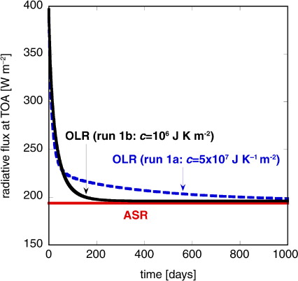
In runs 1a–1f (), the obliquity is set to zero. The model is initialised with an isothermal atmosphere (290 K) at rest. The model atmosphere evolves toward a steady state. The rate of approach to this steady state depends strongly on the value of the thermal inertia coefficient, C (eq. 15). In , the domain-average absorbed solar radiation at the TOA and the domain-average outgoing long wave radiation at the TOA are plotted as a function of time for two values of C. Run 1b, with the lower value of C (=106 J K−1 m−2), reaches equilibrium within 1 yr, while run 1a, with the higher value of C (=5×10⁷ J K−1 m−2), is near to equilibrium after 2–3 yr. With an active water cycle (section 6) the response is accelerated. For our purpose, the model in the permanent equinox runs is sufficiently close to equilibrium after 3 yr (1095 d) of simulation.
Fig. 8 Global average absorbed solar radiation at the top of the atmosphere and global average outgoing long wave radiation at the top of the atmosphere in runs 1a and 1b, which differ only in the value of the thermal inertia coefficient, C.
shows the steady state distribution of potential temperature, zonal wind and wave drag as a function of pressure and latitude for two permanent equinox simulations, one (run 1a; left panel) excluding wave drag and the other (run 1c; right panel) including wave drag. Also shown is the dynamical tropopause, defined in section 2. In the simulation without wave drag the extra-tropics are dominated by one eastward jet, which is consistent with the prediction made at the end of section 3 on the basis of the ‘radiatively determined’ PV. The dynamical tropopause slopes downward gradually from about 100 hPa at 10° latitude to approximately 400 hPa at the poles. The isentropes slope downwards toward the equator at all heights. Again, this is consistent with the ‘radiatively determined’ state (right panel of ), implying that a cold point tropical tropopause is absent.
Fig. 9 Permanent equinox equilibrium state without (run 1a, left panel) and with (run 1c, right panel) wave drag, in an atmosphere lacking water (). Isentropes are labelled in units of K (blue: Underworld; cyan: Middleworld; red: Overworld), zonal wind (u) (black; labelled in units of m s−1; contour interval is 5 m s−1), wave drag, D [eq. (25)] (the dotted line corresponds to D= − 2.5×10⁻⁵ m s−2) and the dynamical tropopause (green line, labelled in PVU), as a function of latitude and pressure. Due to symmetry around the equator, only the northern hemisphere is shown.
![Fig. 9 Permanent equinox equilibrium state without (run 1a, left panel) and with (run 1c, right panel) wave drag, in an atmosphere lacking water (Table 2). Isentropes are labelled in units of K (blue: Underworld; cyan: Middleworld; red: Overworld), zonal wind (u) (black; labelled in units of m s−1; contour interval is 5 m s−1), wave drag, D [eq. (25)] (the dotted line corresponds to D= − 2.5×10⁻⁵ m s−2) and the dynamical tropopause (green line, labelled in PVU), as a function of latitude and pressure. Due to symmetry around the equator, only the northern hemisphere is shown.](/cms/asset/59741254-38fc-4c22-8f9c-9b404977c779/zela_a_11817037_f0009_ob.jpg)
The atmosphere responds to wave drag by producing an adiabatic meridional circulation, which is upward in the tropics and downward in the extra-tropics. Indeed, both the 315 K isentrope and the 370 K isentrope are raised in the tropics and depressed in the extra-tropics due to the effect of wave drag (compare the panels in ). The 750 K isentrope, which is above the maximum height, z 1, of the wave drag [eq. (28)], is not or hardly affected by wave drag. This is an illustration of the ‘downward control’ principle (Haynes et al., Citation1991). Below the level of maximum wave drag, the adiabatic response to wave drag is to drive the temperature away from the ‘radiatively determined’ temperature. The radiative (diabatic) response consists of a diabatic meridional circulation with net radiative heating (cooling) in the tropics (extra-tropics). This translates into cross-isentropic upwelling (downwelling) and convergence (divergence) of mass into the tropical (extra-tropical) Middleworld. This important physical process is analysed further in the following section, after introducing the water cycle.
The ±2 PVU PV-isopleth (the dynamical tropopause) in these simulations seems a rather arbitrary contour, except for the fact that it lies in the region separating the optically thin upper part of the atmosphere and the optically thick lower part of the atmosphere. The optically thin part of the atmosphere, where δ<<1 [eq. (13)], which in this section corresponds to p<<550 hPa, is characterised by nearly isothermal conditions. This is typical for a stratosphere, which is not heated by absorption of solar radiation. By taking account of latent heating due to condensation of water vapour in the layer below 200 hPa in the tropics (next section), the simulated tropical troposphere will be given an important characteristic of the real tropical troposphere, which is part of the Middleworld (). In fact, the Middleworld derives its identity from the large difference in diabatic heating between the tropics and the extratropics, which is the fundamental reason for the large meridional isentropic PV-gradient in the subtropics in this layer. This PV-gradient coincides approximately with the ±2 PVU PV-isopleth. If the question of the origin of the dynamical tropopause is identified with the question of the origin of the almost piecewise uniform nature of the PV field on Middleworld isentropes (Ambaum, 1997), the model results discussed in sections 6–8, might provide at least a partial answer to this question.
6. Permanent equinox in the presence of the water cycle
In this section, a parametrisation of the water cycle is described. The model atmosphere now contains two greenhouse gases: a well-mixed greenhouse gas, as in the previous section (runs 1a–1c, ), and a greenhouse gas which represents water vapour, whose density, ρ
v
, is described by29
where H v is a vertical scale height, assumed to be equal to 2100 m, in accord with observations (Weaver and Ramanathan, Citation1995).
The density of water vapour at the earth's surface, ρ
v
(0), is determined by a prescribed relative humidity at the earth's surface (RH
g
), using the Clausius–Clapeyron equation and the temperature, T
g
, at the earth's surface. It is easily shown, by integrating eq. (29) and assuming that water vapour is an ideal gas, that precipitable water, PW, is related to the surface water vapour density and the scale height by30
where e s (T g ) is the saturation vapour pressure at the earth's surface and R v is the specific gas constant for water vapour. Therefore, precipitable water depends on temperature and relative humidity at the earth's surface.
The long wave optical path, δ, of a model layer is now determined by31
where dp is the layer thickness in Pa, q m and q v are specific concentrations of, respectively, the well-mixed greenhouse gas and of water vapour, and σ m and σ v are the associated absorption cross-sections, which are assumed constant (σ m =0.3 m2 kg−1, as in section 3, and σ v =0.125 m2 kg−1).
At the heart of the parametrisation scheme of the water cycle are the energy fluxes associated with evaporation of water at the surface and condensation of water vapour above cloud base in the atmosphere. These fluxes are prescribed such that energy is conserved. A simple approach to incorporating the energetics of the water cycle into the model, while avoiding explicit modelling of the meridional transport of water vapour through the atmosphere, is to assume that all precipitated water is instantaneously in balance with all evaporated water and that a prescribed fraction (F lp) of the evaporated water condenses and precipitates locally, i.e. at the latitude where it evaporates. Condensation is prescribed according to a prescribed weighting function of pressure. The remainder of the evaporated water converges into a region around the central latitude, y=y ITCZ, of the ITCZ.
Let the precipitation at the central latitude of the ITCZ be P
ITCZ (kg m−2 s−1). The total latent heat, which is released in clouds at this central latitude is L
v
P
ITCZ (W m−2), where L
v
is the latent heat of condensation (2.5×10⁶ J kg−1). This heat is ‘distributed’ over a layer between cloud base (at pressure p=p
cb
) and cloud top (at pressure p=p
ct
), according to a weighting function32
The integral of w(p) from cloud top to cloud base is equal to 1. This distribution function probably overestimates the height of the level of maximum latent heat release, which in reality is much closer to cloud base than to cloud top.
When water vapour condenses, it releases latent heat and precipitates immediately. The diabatic heating in a particular model layer between the pressures p and p+Δp, due to latent heat release, is33
where P is the precipitation in kg s−1 m−2, which is falling out of this particular atmospheric layer and has also condensed in this particular layer.
Latent heating [which contributes to J in eq. (17)] in the ITCZ is distributed in the meridional direction according to the Gaussian function,34
Here, r ITCZ represents the meridional scale of the ITCZ.
The relation between the precipitation, P
ITCZ at y= y
ITCZ, due to convergence of water vapour into the region around the ITCZ, and water, which is evaporated elsewhere, is (neglecting the effect of the convergence of the meridians)35
where E is the evaporated water at the surface (kg m−2 s−1).
E is related to the surface sensible heat flux, H, by a prescribed Bowen ratio,36
This value is consistent with the latest estimate, due to Stephens et al. (Citation2012), of the global average fluxes of surface sensible (24±7 W m−2) and of latent heat (88±10 W m−2). Precipitation at any latitude, y, can be calculated from37
In this way, total evaporation and total precipitation in the model are instantaneously equal to each other and also constrained by the availability of energy at the surface. The net radiation at the surface determines the pace of the water cycle, as it presumably does in reality.
The central latitude of the ITCZ undergoes a seasonal cycle. This is incorporated into the model by letting38
where t is the time in days, t solstice is the time of solstice in the northern hemisphere summer (day 172 or 21 June), a is the radius of the earth and φ max is the latitude (°) of maximum advance toward the pole of the ITCZ. If the ITCZ follows the overhead Sun exactly, φ max, is identical to the obliquity, δ max. In reality, however, φ max<δ max (). This is taken into account by letting δ max=10° in several runs. Moreover, there is a significant delay of about one month or more between the declination angle, δ, of the Sun and the central latitude of the ITCZ. This effect is not taken into account here.
The cloud top pressure depends on latitude as follows.39
Here, p ct0=400 hPa. The tropical cloud tops in the centre of the ITCZ are at 200 hPa, so that Δp ct =−200 hPa. Cloud base is at 900 hPa at all latitudes. The values of the parameters, which are related to the water cycle, are given in .
Table 3. The values and units of model parameters associated with the water cycle
We assume that the interaction of radiation with clouds does not determine the most robust and basic properties of the zonal mean state of the atmosphere, such as the isentropic density in the Middleworld. Therefore, clouds in the model are not radiatively active. In other words, the albedo is not influenced by the presence of clouds, nor do clouds interact with long wave radiation. This assumption is justified a posteriori by the success of the model.
Diabatic heating, J, in the model is the result of absorption of short wave (solar) radiation by the earth's surface and by ozone and water vapour in the atmosphere, of absorption and emission of long wave radiation by greenhouse gases, of evaporation of water at the earth's surface and of latent heat release due to condensation of water vapour in the atmosphere.
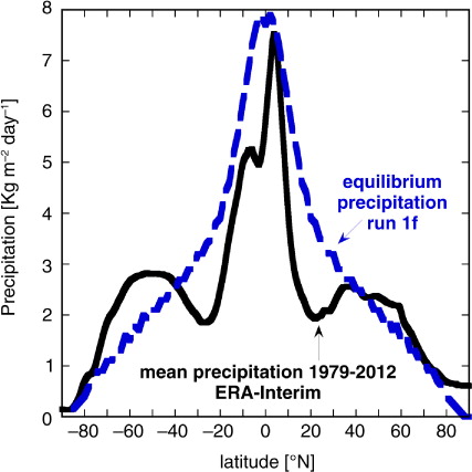
Under permanent equinox conditions (δ max=φ max=0°), an approximate steady state is reached within 2 yr of integration in runs 1d, 1e and 1f (), which include the water cycle. Run 1d, which excludes wave drag, does not produce the tropical upward bulge of the 370 K isentrope. Wave drag is necessary to produce this feature. Runs 1e and 1f, indeed, produce very realistic results. Strictly speaking, the integral of precipitation on a curved surface (i.e. the earth) cannot be compared exactly to the integral of precipitation on a model surface, which neglects the convergence of the meridians. Nevertheless, if we do, we find that the modelled global average steady state precipitation in run 1f (3.4 kg m−2 day−1) compares reasonably well with the ERA-Interim global average precipitation (3.0 kg m−2 day−1) for the period 1979–2012. The dominant tropical maximum at the ITCZ is reproduced quite well (). However, the subtropical minima and the much weaker middle latitude maxima are not reproduced, as expected.
Fig. 10 Zonal mean precipitation, averaged for the years 1979–2012, according to the ERA-Interim re-analysis (Dee et al., Citation2011), as a function of latitude (solid line), and the equilibrium precipitation in run 1f (dashed line).
Despite these shortcomings, the dynamical response to the water cycle leads to significant improvements in the performance of the model in reproducing the important observed features of the zonal mean state. The left panel of shows the modelled steady state potential temperature, zonal wind and wave drag as a function of pressure and latitude under permanent equinox conditions for run 1f. A realistic subtropical jet emerges together with a tropical cold layer at about 100 hPa, as in the annual mean ‘COSPAR International Reference Atmosphere’ (CIRA) (). Animations of runs 1f and 4a are included in the supplementary file. The westward winds in the tropical stratosphere, seen in the annual mean CIRA, are a direct result of the seasonal cycle of the cross-equatorial Hadley cell and hence are not produced in the permanent equinox simulation. The vertical position of the dynamical tropopause, although slightly too low in the extra-tropics and slightly too high in the tropics in terms of pressure, is reproduced satisfactorily in run 1f. The height of the dynamical tropopause is not greatly affected by latent heat release (compare the right panel of with the left panel of ).
Fig. 11 Permanent equinox equilibrium state in run 1f, including wave drag and the water cycle (). Left panel: potential temperature, zonal wind and wave drag as a function of latitude and pressure. Isentropes are labelled in units of K (blue: Underworld; cyan: Middleworld; red: Overworld), zonal wind (u) (black lines, labelled in units of m s−1; contour interval is 5 m s−1), wave drag, D [eq. (25)] (the dotted line corresponds to D=− 2.5×10⁻⁵ m s−2) and the dynamical tropopause, shown in green (labelled in PVU). Right panel: cross-isentropic flow (labelled in units of K day−1; blue: downwelling; red: upwelling) and pressure (dotted lines labelled in units of hPa) as a function of latitude and potential temperature. Due to symmetry around the equator, only the northern hemisphere is shown. Animations of run 1f can be viewed in the supplementary file.
![Fig. 11 Permanent equinox equilibrium state in run 1f, including wave drag and the water cycle (Table 2). Left panel: potential temperature, zonal wind and wave drag as a function of latitude and pressure. Isentropes are labelled in units of K (blue: Underworld; cyan: Middleworld; red: Overworld), zonal wind (u) (black lines, labelled in units of m s−1; contour interval is 5 m s−1), wave drag, D [eq. (25)] (the dotted line corresponds to D=− 2.5×10⁻⁵ m s−2) and the dynamical tropopause, shown in green (labelled in PVU). Right panel: cross-isentropic flow (labelled in units of K day−1; blue: downwelling; red: upwelling) and pressure (dotted lines labelled in units of hPa) as a function of latitude and potential temperature. Due to symmetry around the equator, only the northern hemisphere is shown. Animations of run 1f can be viewed in the supplementary file.](/cms/asset/5c15344a-fa32-40df-8ff6-5dd7df3a7ad3/zela_a_11817037_f0011_ob.jpg)
Fig. 12 The CIRA-annual mean state in terms of potential temperature, labelled in K (blue: Underworld; cyan: Middleworld; red: Overworld), and zonal mean zonal wind (black contours, labelled in m/s) as a function of latitude and pressure. The green contour represents the dynamical tropopause (labelled in PVU).

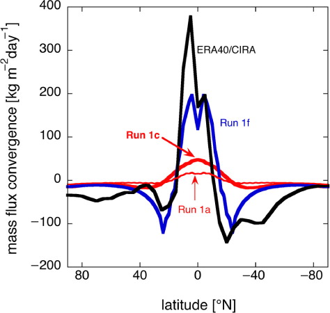
The right panel of shows the steady state cross-isentropic flow in run 1f. This includes the contributions of latent heat release and radiation flux divergence. Comparing this with , we recognise the relatively narrow cross-isentropic upwelling area in the tropical Middleworld, which seems to fan outwards in the lower tropical stratosphere. In the stratosphere, the intensity of the cross-isentropic flow is significantly stronger in the model than in the re-analysis. The combined effect of wave drag in the lower stratosphere and latent heat release in the ITCZ, which in these runs is centred permanently over the equator, is to produce a realistic mass- or isentropic density distribution, especially in the layer of interest between θ=315 K and θ=370 K. This is reiterated in , which compares the steady state net diabatic mass flux, I d [eq. (8)], into the layer between θ=315 K and θ=370 K in runs 1a, 1c and 1f with an estimate of the annual mean of I d in reality (see also ). In run 1a (no wave drag; no water cycle) I d is very small. The physics of this simulation comes closest to the physics of the classical model of the Hadley circulation, due to Held and Hou (Citation1980). In the other two simulations the two cells of the diabatic Hadley circulation can be recognised much more clearly. The maximum value of I d is largest in run 1f, which includes the water cycle. The estimated maximum yearly mean value of I d in reality is even larger. Nevertheless, the qualitative aspects of the latitude dependence of I d are reproduced fairly well in run 1f.
Fig. 13 Steady state diabatic mass flux convergence per unit horizontal area into the Middleworld layer between θ=315 K and θ=370 K as a function of latitude, in the permanent equinox runs 1a, 1c and 1f (), as well as an estimate of the annual mean of this quantity in reality, based on the ERA-40 re-analysis ().
7. The Middleworld PV-budget in the model
In the zonally symmetric setting of the model, the PV-budget eq. (11) becomes40
Here we inspect the PV-budget in the permanent equinox run 1f on the central Middleworld isentrope at θ=350 K. The initial PV-distribution is such that Z=Z ref, so that Z′=0 everywhere. illustrates that an ex-UTLS PV-anomaly and an associated subtropical jet of appreciable amplitude are formed at θ=350 K during the first 50 d of run 1f ().
Fig. 14 Latitude dependence at θ=350 K of the zonal wind (black) and of the PV-anomaly, Z′, [eq. (5)] (blue) on day 10 and day 50 of run 1f ().
![Fig. 14 Latitude dependence at θ=350 K of the zonal wind (black) and of the PV-anomaly, Z′, [eq. (5)] (blue) on day 10 and day 50 of run 1f (Table 2).](/cms/asset/774b25dc-522a-4d91-b6b3-bf16024d6c5e/zela_a_11817037_f0014_ob.jpg)
The first three, of the five, terms on the r.h.s. of eq. (40) afford a straightforward physical interpretation. They represent the influence of (1) isentropic mass flux divergence, (2) cross-isentropic mass flux divergence and (3) isentropic PVS flux convergence. The fourth and fifth terms represent the contribution to the isentropic flux convergence of PVS from the local rate of diabatic heating and from drag. In the model explicit drag is either due to Rayleigh friction, principally below p=700 hPa [eq. (23)], or due to wave drag above z=10 km. Numerical diffusion and smoothing may also play a role here (Plumb and Eluszkiewicz, Citation1999).
Initially, the PV-budget at θ=350 K in run 1f is determined by divergence of cross-isentropic mass transport, but within a few days isentropic divergence of mass and PVS in the Hadley circulation also contribute to the local PV-budget at this level.
displays the magnitudes of the first three PV-source terms [eq. (40)] at θ=350 K as a function of latitude on day 25 of run 1f. The magnitudes of the fourth and fifth terms are negligible at this level, as can be verified by comparing the sum of all five terms with first three terms individually. The atmosphere in this stage is not yet in equilibrium (). Equatorward of φ=±25° the PV-budget is effectively determined by isentropic flux convergence of PVS [the third term on the r.h.s. of eq. (40)] in the upper branch of the Hadley circulation, since cross-isentropic mass flux divergence [the second term on the r.h.s. of eq. (40)] is almost exactly compensated by isentropic mass flux divergence [the first term on the r.h.s. of eq. (40)]. Negative PVS flux convergence on the equatorward flank of the subtropical jet produces anticyclonic vorticity, while positive PVS flux convergence on the poleward flank of the subtropical jet produces cyclonic vorticity.
Fig. 15 Latitude dependence at θ=350 K of the zonal wind (solid black) and of the first three PV-source terms on the r.h.s. of eq. (40) on day 25 of the permanent equinox run 1f (). The grey dashed line represents the sum of all five terms on the r.h.s. of eq. (40).
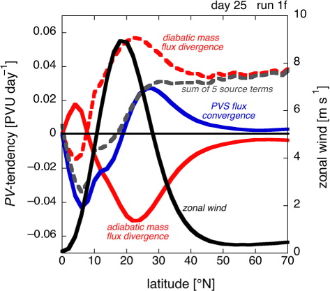
In the extratropical Middleworld, positive cross-isentropic mass flux divergence, associated with downwelling cross-isentropic flow, dominates the PV-budget (). This effect is responsible for an increase of PV poleward of 45° latitude. Therefore, the high latitude portion of the ‘ex-UTLS PV-anomaly’ is formed by diabatic mass flux divergence, while the low latitude portion is formed by isentropic PVS-flux convergence in the upper branch of the Hadley circulation.
8. Results of simulations of the seasonal cycle
The credibility of the model is convincingly demonstrated by the results of simulations including the seasonal cycle, which are discussed in this section. The seasonal cycle is introduced by setting the obliquity, δ max, at the present day value of 23.45°. The latitude of maximum poleward advance of the ITCZ, φ max, is either 23.45°, in which case the ITCZ follows the overhead position of the Sun (runs 2a–c and 3a–d), or 10°, which is more realistic (runs 4a–b). Runs 2a–c (), which are intended to test the effect of ozone in relation to the effect of wave drag on the seasonal cycle of the zonal wind, excluding the effect of the water cycle, demonstrate that wave drag is needed to obtain a realistic seasonal cycle of the zonal wind. Without wave drag, but including ozone, the model does not produce the spring zonal wind reversal in the extra-tropical stratosphere. With wave drag it does.
This is further corroborated by the results of runs 3a and 3b, which include the water cycle. Again, without wave drag (run 3a) a zonal wind reversal does not occur, while it does occur with wave drag (right panel of ). Wave drag in the model induces a negative polar cap PV-anomaly in winter in the layer between θ=380 K and θ=500 (left panel of ), in agreement with reality (). The ex-UTLS PV-anomaly in run 3b is centred permanently at approximately θ=335 K, but is somewhat weaker and appears smoothed vertically in comparison to reality.
Fig. 16 As in , but for year 3 of run 3b. Labels in left panel are in units of PVU. Labels in right panel are in are in units of m s−1.
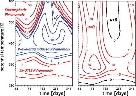
The negative polar cap PV-anomaly in run 3b expands upward relatively slowly in spring, ultimately inducing a reversal of the stratospheric zonal wind. In reality the reversal of the sign of the polar cap PV-anomaly in spring occurs nearly simultaneously at all levels above θ=550 K () (see also Hinssen et al., 2011a). The negative polar cap PV-anomaly in the surf zone in reality forms due to meridional mixing of (reference) PV by planetary waves. The wave drag parametrisation has an identical qualitative effect on the PV-distribution and hence serves as a surrogate for meridional PV-mixing.
The date of the spring/summer wind reversal, which occurs about 10 d after solstice in run 3b, i.e. at least one (or two) months later than the observed average time of wind reversal in the southern (northern) hemisphere, depends both on the magnitude of the wave drag and the coefficient of thermal inertia, C. A lower value of C, keeping the wave drag coefficient, D 0, constant (run 3d), leads to an earlier spring stratospheric wind reversal. This implies that conditions at the earth's surface influence the circulation in the stratosphere, as is observed in .
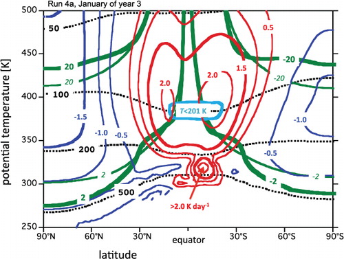
shows the January average PV, cross-isentropic flow, pressure and temperature in year 3 of the most realistic simulation (run 4a), in which φ max=10. Comparison with reveals that the diabatic circulation and pressure- and PV distributions are reproduced quite well, qualitatively. The lower atmosphere in the model is too cold. The height of the tropical cold point at about 100 hPa is reproduced quite accurately, but its temperature (200 K) is 10 K higher than observed (Randel and Jensen, Citation2013). The stratospheric part of the diabatic circulation is stronger in the model than in the ERA-40 re-analysis, but its main features, such as the meridional broadening of the tropical cross-isentropic upwelling in the stratosphere is fairly well reproduced, although this meridional broadening is, in contrast to reality, already observed somewhat below the cold point tropical tropopause in the model. Animations of run 4a are included in the supplementary file.
Fig. 17 January average in year 3 of run 4a () of zonal mean pressure (dotted black lines, labelled in units of hPa), potential vorticity (thick green lines, labelled in PVU), reference potential vorticity (thin green lines, labelled in PVU), cross-isentropic flow (labelled in units of K day−1; blue: downwelling; red: upwelling) and temperature (cyan; only the 201 K isotherm) as a function of latitude and potential temperature. An animation of run 4a can be viewed in the supplementary file.
9. Conclusion
This paper investigates how the interaction between diabatic components and adiabatic components of the general circulation determines the zonal mean PV-distribution.
Zonal mean PV is determined in the first place by the ‘radiatively determined’ isentropic density, which decreases upward and poleward. The amplitude of the resulting hemispheric-wide ‘radiatively determined’ cyclonic PV-anomaly, centred over the Pole, depends crucially on the time scale of the response to the solar forcing through the annual cycle. This time scale depends on the thermal inertia of both the atmosphere and the earth's surface.
Westward planetary wave drag in the lower stratosphere induces an adiabatic vertical/meridional circulation. Below the level of maximum wave drag, this circulation maintains the temperature in the tropics (extra-tropics) below (above) the ‘radiatively determined’ temperature. The diabatic/radiative response to this disequilibrium is a circulation with cross-isentropic upwelling in the tropics and cross-isentropic downwelling in the extra-tropics. In the tropical troposphere, which is part of the Middleworld, the cross-isentropic upwelling is very strongly intensified by latent heat release.
Because the ‘radiatively determined’ isentropic density decreases with height, cross-isentropic upwelling (downwelling) tends to be associated with cross-isentropic mass flux convergence (divergence). This leads to a decrease (an increase) of PV in the tropics (extratropics), which enhances the amplitude of the existing ‘radiatively determined’ cyclonic PV-anomaly.
This diabatic–dynamical interaction is simulated with a highly simplified two-dimensional (latitude–height) primitive equation model, which includes parametrisations of radiative transfer, dry convective adjustment, wave drag and water cycle. A realistic distribution of cross-isentropic flow below 10 hPa is obtained, with cross-isentropic upwelling in the tropics and cross-isentropic downwelling in the extratropics.
Model simulations demonstrate that the tropical PV-budget in the Middleworld is dictated both by latent heat release in the ITCZ and by radiative cooling in the subtropics and in the extratropics. Mass converges diabatically into the tropical Middleworld above the ITCZ, while mass diverges diabatically out of the Middleworld in the subtropics. These cross-isentropic mass fluxes represent the vertical branches of the ‘diabatic Hadley circulation’. Isentropic PVS flux divergence in the upper isentropic branch of the Hadley circulation in the tropical Middleworld is instrumental in strengthening the meridional PV-gradient in the subtropics, coinciding with the isentropic dynamical tropopause. This translates into a strong subtropical meridional slope of the dynamical tropopause.
The influence of wave drag on the PV-budget is recognised in the negative polar cap PV-anomaly in the layer between θ=390 K and θ=550 K (see the left panel of ). In the model (left panel of ), this PV-feature arises due to two effects: (1) due to the wave drag induced equatorward flux of PVS, and (2) due to the wave drag induced isentropic poleward mass flux.
At levels above about θ=550 K (about 50 hPa) cross-isentropic up- or downwelling presumably dominates the isentropic mass budget and hence also dictates the PV-budget. This is because of high radiative cooling rates in winter in combination with (probably) weaker wave drag (except during sudden stratospheric warmings), and because of the high diabatic heating rates in summer in connection with absorption of solar radiation by ozone.
shows the annual mean state in year 3 of run 4a. It should be remarked that this solution is quite sensitive to the amplitude of wave drag (the value of D 0) and the thermal inertia of the earth's surface (the value of C). Because differences in wave drag and in heat capacity of the earth's surface between the two hemispheres are not taken into account, the modelled annual average state is practically symmetric about the equator, which is in contrast to reality (). Nevertheless confidence in the model is boosted by the fact that it qualitatively reproduces many observed features of the annual mean zonal mean state of the atmosphere. This includes the jets, a realistic distribution of cross-isentropic flow, the tropical cold point and the associated tropical upward bulge of the 370 K isentrope, the annual average easterlies in the tropics, the strong slope of the dynamical tropopause in the subtropics and the associated isentropic tropopause in the subtropics at θ=350 K, and the seasonal stratospheric zonal wind reversals, despite some strong simplifications, such as grey long wave radiative transfer, a simplified representation of the water cycle, radiatively inactive clouds, constant surface albedo, constant Bowen ratio and a rather crude parametrisation of wave drag, as a surrogate for meridional isentropic PV-mixing. But precisely because of its simplicity, and because of our confidence in the complete model, we are, by disassembling the model to study the interaction of its parts, able to dissect the interaction between diabatic processes (cross-isentropic flow) and adiabatic processes (isentropic transport of mass and PV substance), and so to recognise what causes what. The central role in this interaction of planetary wave drag and the insecure footing of the wave drag parametrisation in theory calls for further research efforts to better understand this role.
Fig. 18 Annual mean state in year 3 in run 4a () in terms of potential temperature, labelled in K (blue: Underworld; cyan: Middleworld; red: Overworld), and zonal wind (black), labelled in m/s, as a function of latitude and pressure. The green contour represents the dynamical tropopause (labelled in PVU). An animation of run 4a can be viewed in the supplementary file.
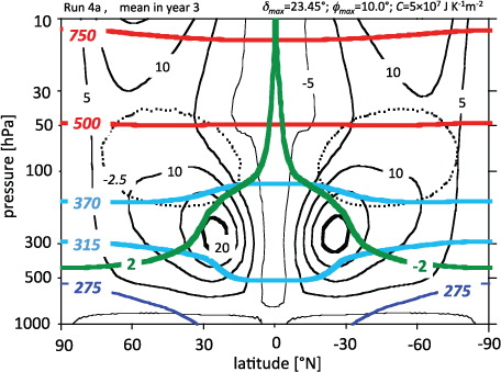
Figure 11, left run 1f
Download (2.4 MB)Figure 11, right run 1f
Download (2.5 MB)Figure 17, run 4a
Download (2.4 MB)Figure 18, run 4a
Download (2.5 MB)Supplementary material - legends
Download MS Word (26.5 KB)10. Acknowledgements
I wish to thank the three reviewers for very useful comments and criticism, Paul Berrisford for providing the ERA-40 diabatic heating data, Koen Manders, Niels Zweers and Roos de Wit for help in developing and debugging the numerical model and for stimulating scientific input in the early stages of this research project, Yvonne Hinssen and Theo Opsteegh for very useful discussions on potential vorticity inversion, Bruce Denby for his large contribution in developing the computer graphics, the students of my course on climate and the water cycle for inspiration and useful suggestions on incorporating and validating the parametrisations associated with the water cycle, Marcel Portanger for advice and help on computer problems and, finally, all my colleagues at IMAU for allowing me to work on such a large and time-consuming project.
Notes
To access the supplementary material to this article, please see Supplementary files under Article Tools online.
Related Research Data
References
- Ambaum M . Isentropic formation of the tropopause. J. Atmos. Sci. 1997; 54: 555–568.
- Charney J. G. , Drazin P . Propagation of planetary scale disturbances from the lower atmosphere into the upper atmosphere. J. Geophys. Res. 1961; 66: 83–109.
- Dee D. P. , Uppala S. M. , Simmons A. J. , Berrisford P. , Poli P. , co-authors . The ERA-Interim reanalysis: configuration and performance of the data assimilation system. Q. J. R. Meteorol. Soc. 2011; 137: 553–597.
- Edouard S. , Vautard R. , Brunet G . On the maintenance of potential vorticity in isentropic coordinates. Q. J. R. Meteorol. Soc. 1997; 123: 2069–2094.
- Fels S. B . Radiative–dynamical interactions in the middle atmosphere. Adv. Geophys. 1985; 28A: 277–300.
- Fels S. B. , Mahlman J. D. , Schwarzkopf M. D. , Sinclair R. W . Stratospheric sensitivity to perturbations in ozone and carbon dioxide: radiative and dynamical response. J. Atmos. Sci. 1980; 37: 2265–2297.
- Fleming E. L. , Chandra S. , Barnett J. J. , Corney M . Zonal mean temperature, pressure, zonal wind, and geopotential height as functions of latitude. Adv. Space. Res. 1990; 10(12): 11–59.
- Fortuin J. P. F. , Kelder H . An ozone climatology based on ozonesonde and satellite measurements. J. Geoph. Res. 1998; 103: 31709–31734.
- Fueglistaler S. , Legras B. , Beljaars A. , Morcrette J.-J. , Simmons A. , co-authors . Diabatic heat budget of the upper troposphere and lower/mid stratosphere in ECMWF reanalyses. Q. J. R. Meteorol. Soc. 2009; 135: 21–37.
- Gettelman A. , Hoor P. , Pan L. L. , Randel W. J. , Hegglin M. I. , co-authors . The extratropical upper troposphere and lower stratosphere. Rev. Geophys. 2011; 49: RG3003.
- Hartmann D. L . The atmospheric general circulation and its variability. J. Meteorol. Soc. Japan. 2007; 85B: 123–143.
- Haynes P. H. , Marks C. J. , McIntyre M. E. , Shepherd T. G. , Shine K. P . On the “downward control” of extratropical diabatic circulations by eddy-induced mean zonal forces. J. Atmos. Sci. 1991; 48: 651–678.
- Haynes P. H. , McIntyre M. E . On the evolution of vorticity and potential vorticity in the presence of diabatic heating and frictional or other forces. J. Atmos. Sci. 1987; 44: 828–841.
- Haynes P. H. , McIntyre M. E . On the conservation and impermeability theorems for potential vorticity. J. Atmos. Sci. 1990; 47: 2012–2031.
- Haynes P. H. , McIntyre M. E. , Shepherd T. G . Reply to a comment by J. Egger. J. Atmos. Sci. 1996; 53: 2105–2107.
- Held I. M. , Hou A. Y . Nonlinear axially symmetric circulations in a nearly inviscid atmosphere. J. Atmos. Sci. 1980; 37: 515–533.
- Held I. M. , Suarez M. J . A proposal for the intercomparison of the dynamical cores of atmospheric general circulation models. Bull. Amer. Meteorol. Soc. 1994; 75: 1825–1830.
- Highwood E. J. , Hoskins B. J . The tropical tropopause. Quart. J. R. Meteorol. Soc. 1998; 124: 1579–1604.
- Hinssen Y. , van Delden A. , Opsteegh J . Influence of sudden stratospheric warmings on the tropospheric winds. Meteorol. Z. 2011a; 20: 259–266.
- Hinssen Y. , van Delden A. , Opsteegh J. , de Geus W . Stratospheric impact on the troposphere deduced from potential vorticity inversion in relation to the Arctic Oscillation. Quart. J. R. Meteorol. Soc. 2010; 136: 20–29. See also the corrigendum: Quart. J. R. Meteorol. Soc. 136, 2203–2204.
- Hinssen Y. B. L. , Ambaum M. H. P . Relation between the 100 hPa heat flux and stratospheric potential vorticity. J. Atmos. Sci. 2010; 67: 4017–4027.
- Hinssen Y. B. L. , Bell C. J. , Siegmund P. C . The influence of the stratosphere on the tropospheric zonal wind response to CO2 doubling. Atmos. Chem. Phys. 2011b; 11: 4915–4927.
- Hoerling M. P . Diabatic sources of potential vorticity in the general circulation. J. Atmos. Sci. 1992; 49: 2282–2292.
- Hoskins B. J . Towards a PV-θ view of the general circulation. Tellus B. 1991; 43: 27–35.
- Holton J. R . An Introduction to Dynamic Meteorology.
- Koshyk J. N. , McFarlane N. A . The potential vorticity budget of an atmospheric general circulation model. J. Atmos. Sci. 1996; 53: 550–563.
- Manabe S. , Hunt B. G . Experiments with a stratospheric general circulation model. 1. Radiative and dynamic aspects. Mon. Wea. Rev. 1968; 96: 477–502.
- Manabe S. , Mahlman J. D . Simulation of seasonal and interhemispheric variations in the stratospheric circulation. J. Atmos. Sci. 1976; 33: 2185–2217.
- Manabe S. , Smagorinsky J. , Strickler R. F . Simulated climatology of a general circulation model with a hydrological cycle. Mon. Wea. Rev. 1965; 93: 769–798.
- McIntyre M. E. , Palmer T. N . The “surf zone” in the stratosphere. J. Atmos. Terr. Phys. 1984; 46: 825–849.
- Mendez-Nunez L. R. , Caroll J. J . Comparison of leapfrog, Smolarkiewicz, and MacCormack schemes applied to nonlinear equations. Mon. Wea. Rev. 1993; 121: 565–578.
- Pawson S. , Kodera S. , Hamilton K. , Shepherd T.G. , Beagley R. , co-authors . The GCM-reality intercomparison project for SPARC (GRIPS): scientific issues and initial results. Bull. Amer. Meteorol. Soc. 2000; 81: 781–796.
- Pierrehumbert R. T . Principles of Planetary Climate.
- Plumb R. A. , Eluszkiewicz J . The Brewer-Dobson circulation: dynamics of the tropical upwelling. J. Atmos. Sci. 1999; 56: 868–890.
- Randel W. J. , Jensen E. J . Physical processes in the tropical tropopause layer and their roles in a changing climate. Nat. Geosci. 2013; 6: 169–176.
- Schumacher C. , Houzeand R. A. , Kraucunas I . The dynamical response to latent heating estimates derived from the TRMM precipitation radar. J. Atmos. Sci. 2004; 61: 1341–1358.
- Semeniuk K. , Shepherd T. G . The middle atmosphere Hadley circulation and equatorial inertial adjustment. J. Atmos. Sci. 2001; 58: 3077–3096.
- Shapiro R . Smoothing, filtering and boundary effects. Rev. Geophys. Space Phys. 1970; 8: 359–387.
- Shaw N . Manual of Meteorology. 1931; Cambridge University Press, London.
- Smagorinsky J . Some aspects of the general circulation. Q. J. R. Meteorol. Soc. 1964; 90: 1–14.
- Smagorinsky J. , Manabe S. , Holloway Jr J. L . Numerical results from a nine-level general circulation model of the atmosphere. Mon. Wea. Rev. 1965; 93: 727–768.
- Stephens G. L. , Li J. , Wild M. , Clayson C. A. , Loeb N. , co-authors . An update on earth's energy balance in light of the latest global observations. Nat. Geosci. 2012; 5: 691–696.
- Strauss D. M. , Shukla J . A comparison of a GCM simulation of the seasonal cycle of the atmosphere with observations. Part 1: mean fields and the annual harmonic. Atmos. Ocean. 1988; 26: 541–574.
- Uppala S. M. , Kallberg P. W. , Simmons A. J. , Andrae U. , Da Costa Bechtold V. , co-authors . The ERA-40 re-analysis. Q. J. R. Meteorol. Soc. 2005; 131: 2961–3012.
- Van Delden A. J. , Hinssen Y. B. L . PV-theta view of the zonal mean state of the atmosphere. Tellus A. 2012; 64: 18710. DOI: 10.3402/tellusa.v64i0.18710.
- Washington W. M. , Parkinson C. L . An Introduction to Three-Dimensional Climate Modeling.
- Weaver C. P. , Ramanathan V . Deductions from a simple climate model: factors governing surface temperature and atmospheric thermal structure. J. Geophys. Res. 1995; 100: D6, 11585–11591.