Improving the multiannual, high-resolution modelling of biogeochemical cycles in the Baltic Sea by using data assimilation

Abstract

The impact of assimilating temperature, salinity, oxygen, phosphate and nitrate observations on marine ecosystem modelling is assessed. For this purpose, two 10-yr (1970–1979) reanalyses of the Baltic Sea are carried out using the ensemble optimal interpolation (EnOI) method and a coupled physical-biogeochemical model of the Baltic Sea. To evaluate the reanalyses, climatological data and available biogeochemical and physical in situ observations at monitoring stations are compared with results from simulations with and without data assimilation. In the first reanalysis, only observed temperature and salinity profiles are assimilated, whereas biogeochemical observations are unused. Although simulated temperature and salinity improve considerably as expected, the quality of simulated biogeochemical variables does not improve and deep water nitrate concentrations even worsen. This unexpected behaviour is explained by a lowering of the halocline in the Baltic proper due to the assimilation causing increased oxygen concentrations in the deep water and consequently altered nutrient fluxes. In the second reanalysis, both physical and biogeochemical observations are assimilated and good quality in all variables is found. Hence, we conclude that if a data assimilation method like the EnOI is applied, all available observations should be used to perform reanalyses of high quality for the Baltic Sea biogeochemical state estimates.

• reanalysis
• data assimilation
• numerical modelling
• Baltic Sea
• biogeochemical simulation

1. Introduction

Numerical modelling is used as a complement in environmental impact assessments and for investigations, for example, of the Baltic Sea (Fig. 1) nutrient cycling and nutrient reduction scenarios (e.g. Eilola et al., 2012; Meier et al., 2012; Neumann et al., 2012; Omstedt et al., 2012). Ecological and biogeochemical models with varying levels of complexity are under continuous evolution, and recently a coupled high-resolution three-dimensional (3D) models including also the North Sea are developed at the Swedish Meteorological and Hydrological Institute (SMHI) (Kuznetsov et al., manuscript in preparation) and other institutes around the Baltic Sea (Maar et al., 2011; Daewel and Schrum, 2013). In addition to the ecosystem model development, comprehensive historical data sets are established for the Baltic Sea region based on the joint efforts of all countries bordering the Baltic Sea. For instance, monitoring data are available from the International Council for the Exploration of the Sea (ICES) (http://www.ices.dk), from the Swedish Oceanographic Data Centre (SHARK) (http://www.smhi.se/en/Research/open-access-to-data-for-research-and-development-1.31497) hosted by SMHIand from the Baltic Nest Institute (BNI) (http://www.balticnest.org) hosting the partnership of systems of distributed databases where each partner (see http://nest.su.se/bed/hydro_chem.shtml) makes the data stored in its databases publicly available. Near real-time observations are also available by the partners participating in the Baltic Sea Operational Oceanographic System (BOOS) (http://www.boos.org/).

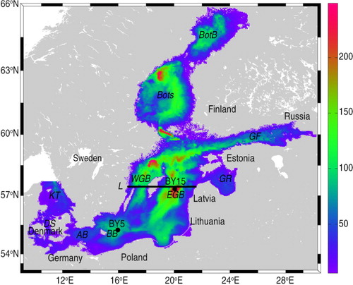
Fig. 1 The bathymetry of the RCO model (depths in m). The positions of selected monitoring stations, BY15 (57.33°N, 20.05°E) and BY5 (55.25°N, 15.98°E), are indicated by black dots and the position of the section L (along 57.44°N) is shown by the black line. Various subbasins in the Baltic Sea are Kattegat (KT), Danish straits (DS), Arkona Basin (AB), Bornholm Basin (BB), eastern Gotland Basin (EGB), western Gotland Basin (WGB), Gulf of Riga (GR), Gulf of Finland (GF), Bothnian Sea (BotS) and Bothnian Bay (BotB).

These observations provide an important tool to validate the model results and identify shortcomings of the ecosystem models that need to be further developed. Three state-of-the-art physical-biogeochemical models of the Baltic Sea, including the high-resolution Rossby Centre Ocean model (RCO) coupled to the Swedish Coastal and Ocean Biogeochemical model (SCOBI) that is used in the present paper, were evaluated by Eilola et al. (2011). One of the models in the Eilola et al. (2011) ensemble resolves the Baltic Sea into 13 dynamically interconnected and horizontally integrated subbasins while the RCO-SCOBI model has a resolution of 3.7 km. Hence, the calibrated parameters of the biogeochemical models may differ because of different resolutions of the descriptions of biogeochemical sources and sinks inside the Baltic Sea. These coupled physical-biogeochemical models aim to simulate the ecological and biogeochemical responses of the Baltic Sea to changes in physical conditions and nutrient loadings. Eilola et al. (2011) concluded that the models capture much of the long-term observed variability (1970–2005) in the Baltic proper but showed considerable biases in the northern Baltic Sea. They also found that no model showed outstanding performance in all aspects; instead, the ensemble mean results were found to give the best representation of observations. Possible reasons for uncertainties in the model results were due to model forcing, less well-known process descriptions and initial conditions of the model simulations.

Since all models have to deal with uncertainties due to limitations in forcing and process descriptions, and real measurements are limited by a poor coverage in time and space, methods of data assimilation (Gregg et al., 2009) may provide a synthesis between models and observations. Data assimilation is frequently used in prognostic models for improving the predictive capacity of models. For this aim, many advanced assimilation methods based on the Kalman filter (e.g. EnKF; Evensen, 2003) and variational methods (3DVAR and 4DVAR) (Zhu et al., 2006; Liu and Yan, 2010; Liu and Zhao, 2011) have widely been used in the areas of ocean and atmospheric modelling. The ensemble optimum interpolation (EnOI) method (Fu et al., 2011; Liu et al., 2013) that will be used in this study is similar to the optimum interpolation (OI) method applied for the operational ocean forecasting system at the SMHI (Pemberton and Funkquist, 2006). Assimilation of sea surface temperatures estimated from satellite data (NOAA) is used, for example, in the Baltic operational circulation model presented by Losa et al. (2012, 2014) and recently several data assimilation studies have focused on the historical reanalysis of salinity and temperature in the Baltic Sea (e.g. Fu et al., 2012; Fu, 2013; Liu et al., 2013). As a next step in the development of historical, marine reanalyses, the present paper focuses on the assimilation also of nutrients and oxygen in the Baltic Sea following Liu et al. (2013). The aim with the production of reanalysis data is, inter alia, to support better assessments of historical changes in ecological quality indicators and to improve quantification of nutrients budgets and the extensions of hypoxic and anoxic areas (so-called dead bottoms). We will analyse the effects on the biogeochemistry of assimilating only observed temperature and salinity profiles and compare to results in a situation where both physical and biogeochemical observations are assimilated.

This paper is organised as follows. The RCO and SCOBI models are described in Section 2.1. Then the data assimilation method and the observations are introduced in Sections 2.2 and 2.3, respectively. The experimental design and configurations are described in Section 2.4. In Section 2.5, the quality measure [root mean square deviation (RMSD)] is defined. Results of the experiments including comparisons with observations are presented in Section 3. Finally, in Sections 4 and 5 discussion and conclusions finalise the paper.

2. Methods

2.1. Models

The coupled model system is based on the SCOBI (Eilola et al., 2009) and the RCO (Meier et al., 2003; Meier, 2007). The model domain of RCO-SCOBI mode covers the Baltic Sea with open boundaries in the northern Kattegat. Boundary conditions are based on Stevens (1991) with prescribed sea surface heights. In case of inflow, temperature and salinity variables are nudged towards observed climatological mean profiles. In case of outflow, an Orlanski radiation condition is utilised (Orlanski, 1976). In RCO, a flux corrected transport scheme (Gerdes et al., 1991), a bottom boundary layer model (Beckmann and Döscher, 1997), a two-equation turbulence closure scheme of the k-ɛ type (Meier, 2001) and a Hible-type (Hibler, 1979), multicategory sea ice model (Mårtensson et al., 2012) with elastic-viscous-plastic rheology (Hunke and Dukowicz, 1997) are implemented. The horizontal grid resolution amounts to 2 nautical miles or 3.7 km which is regarded as eddy-permitting. Eighty-three vertical levels with layer thickness of 3 m are used. For further details of the RCO configuration, the reader is referred to Meier et al. (1999, 2003) and Meier (2007).

The biogeochemical model SCOBI is coupled to RCO and describes the dynamics of nutrients (phosphate, nitrate, ammonium), phytoplankton (diatoms, flagellates and others and cyanobacteria), zooplankton, detritus and oxygen. Processes like assimilation, remineralization, nitrogen fixation, nitrification, denitrification, grazing, mortality, excretion, sedimentation, resuspension and burial are considered. With the help of a simplified wave model resuspension of organic matter is calculated from the wave and current induced shear stresses (Almroth-Rosell et al., 2011). The production of phytoplankton assimilates carbon (C), nitrogen (N) and phosphorus (P) according to the Redfield molar ratio (C:N:P=106:16:1) and the biomass is represented by chlorophyll (Chl) according to a constant carbon to chlorophyll ratio C:Chl=50 (mg C/mg CHLa) (Eilola et al., 2009). The molar ratio of a complete oxidation of the remineralized nutrients is O₂:C=138. Therefore, when observations of oxygen and nutrient concentrations are assimilated into the RCO-SCOBI also the primary production rate, the chlorophyll concentrations and the oxygen consumption are affected by the assimilation. For further details of the SCOBI model, the reader is referred to Eilola et al. (2009, 2011) and Almroth-Rosell et al. (2011).

Atmospheric forcing data for the period 1970–1979 are calculated from regionalised ERA-40 data using a regional atmosphere model with a horizontal grid resolution of 25 km (Samuelsson et al., 2011). For the wind speed, a bias correction method following Meier et al. (2011) is applied. The hydrological forcing is based upon monthly mean river runoff observations (Bergström and Carlsson, 1994). Monthly nutrient loads from rivers and point sources and of atmospheric nitrogen deposition are calculated from historical data (Savchuk et al., 2012). Initial conditions for January 1970 are taken from an earlier run with RCO-SCOBI.

The results of the simulation without data assimilation presented in this study differ from earlier presented results by Eilola et al. (2011) because RCO-SCOBI was updated with a higher vertical grid resolution improving the model's capacity to simulate saltwater inflows into the Baltic proper deep water (Matthäus and Franck, 1992). However, the biogeochemical model SCOBI has not been recalibrated to the altered physical conditions of the present version. Hence, for example, the oxygen concentrations in deep waters are lower due to a stronger stratification causing higher PO4 concentrations compared to the version presented by Eilola et al. (2011). A recalibration of SCOBI is out of the scope of the present study. Rather, our focus is on the impact of the assimilation with and without biogeochemical observations.

2.2. Ensemble optimal interpolation

The data assimilation method used in this study is EnOI (Evensen, 2003; Oke et al., 2005), which is developed from EnKF. In theory, EnOI uses a stationary ensemble to approximate the system's background error covariance (BEC). The ensemble of anomalies of states is sampled from model states in long-term simulations. A large ensemble of model states can be used to ensure that EnOI spans a sufficiently large space for a proper analysis. The analysis increments are comprised of a linear combination of model anomalies. EnOI is different from the traditional OI method because traditional OI schemes estimate BECs with the help of simple analytical functions which are used uniformly for the entire model grid. On the other hand, EnKF updates the ensemble mean and the ensemble perturbations during every assimilation cycle. This yields a time-varying estimate of the system's BEC. Relative to EnKF EnOI is inexpensive and robust because it requires only one deterministic model run and only one background state needs to be updated (analogous to the ensemble mean in the EnKF). EnOI has been successfully tested for a wide range of ocean applications (e.g. Counillon and Bertino, 2009; Liu et al., 2013). For further details of the EnOI, the reader is, for instance, referred to Liu et al. (2013).

2.3. Observations

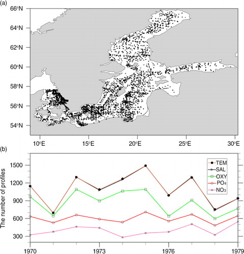
For the assimilation, observations of physical (temperature and salinity) and biogeochemical (oxygen, nitrate and phosphate) variables from SHARK are used. Figure 2 shows the spatial and temporal distribution of these data during 1970–1979. Observations are inhomogeneous in time and space. The available observations of biogeochemical variables are always less than the observations of physical variables in the same year. There are more observations from the Kattegat, Arkona Basin, Bornholm Basin, and Gotland Basin than from other regions. Data from two standard monitoring stations BY5 (55.25°N, 15.98°E) and BY15 (57.33°N, 20.05°E) are used in the analysis (Fig. 1). The depths are about 90 and 250 m, respectively. BY5 is located in the central Bornholm Basin relatively close to the Danish straits. The hydrography at BY15 located further to the east is representative for the entire eastern Gotland Basin.

Fig. 2 Spatial distribution of temperature observations (a) and annual number of temperature, salinity, oxygen, phosphate, and nitrate observations during the 1970–1979 (b).

A gross error check, for instance of location and stability, was made before the data were stored in SHARK. Before the data assimilation, we apply some additional quality controls of the extracted data excluding (1) duplicate observations, (2) observations located on land defined by the RCO-SCOBI model grid and (3) observations with differences to model forecasts exceeding a given threshold. Here, the thresholds for absolute differences in temperature, salinity, oxygen, nitrate and phosphate amount to 3.0°C, 3 psu, 3.0 mL L⁻¹, 4.0 mmol L⁻³ and 3.0 mmol L⁻³, respectively. The exclusion of these data is done because data points that exceed the limits may cause instabilities and too large sudden deviations in the state of the model physics. By the above criteria, about 8% of the observations are discarded. When there is more than one observation per model layer at the same time and same position, we use an average of concerned observations.

In addition, we evaluate the results of the reanalyses with the help of independent, climatological monthly mean gridded data from Janssen et al. (1999).

2.4. Experimental design and configurations

Three 10-yr long simulations for the period from January 1970 to December 1979 were performed. The control run, henceforth called FREE, is a model simulation without data assimilation. Further, two simulations with assimilation of either observed physical variables only (henceforth called REANA) or both observed physical and biogeochemical variables (henceforth called REANAB). In order to clearly show the effect of assimilating the biogeochemical observations at the same physical conditions of REANA, the covariance between physical and biogeochemical variables is omitted in REANAB. The data assimilation is therefore divided into two independent cycles. First, the assimilation of temperature and salinity observations is performed identical to REANA following Liu et al. (2013). After that, the biogeochemical observations are assimilated without any direct influence on physical variables.

Following Liu et al. (2013), we adopt the method of a running selection of samples to obtain a quasi-stationary BEC. At every assimilation cycle, we utilise in total 100 model samples within a 90 d window. The calendar date of the assimilation time is in the centre of the ensemble window. Hence, from every year during the arbitrarily selected period 1964–1968, 20 snapshots have been selected.

To perform localisation, we have chosen a radius of 70 km beyond which the correlations are set to zero. The number is based on previous studies and a set of sensitivity experiments that showed that 70 km is a reasonable length scale for this reanalysis in the Baltic Sea. The adaptive assimilation parameter ‘alpha’ is calculated before each local analysis of the simulation (Liu et al., 2013). In both data assimilation simulations, the time window for choosing observations is 3 d before and after assimilation time and the assimilating frequency is once every 7 d. For simplicity, the observations are considered to be uncorrelated (e.g. Liu et al., 2009). The observation error variances (diagonal elements of observational error covariance matrix) for individual observations are estimated according to the relative ‘age’ of each observation:1 2

where Δt (in days) is the time difference between observation and assimilation occasions. ɛ _T (in °C), ɛ _S (in psu), (in mL L⁻¹), (in mmol L⁻³) and (in mmol L⁻³) are the observations error of temperature, salinity, oxygen, phosphate and nitrate, respectively.

2.5. Root mean square deviations

To evaluate the overall impact of assimilating either physical or biogeochemical observations on biogeochemical variables during 1970–1979, monthly mean RMSDs of temperature, salinity, oxygen, phosphate and nitrate between simulation results in FREE, REANA and REANAB and observations are calculated. The RMSD at one assimilation time is calculated according to:3

where N _t is the number of the observations at one assimilation time. represents the difference between model result and observation. For this evaluation of model simulations, all quality-controlled observations are used. In REANA and REANAB, the δ is calculated just before the assimilation analysis time and the corresponding observations are not yet assimilated into RCO-SCOBI (Liu et al., 2009).

3. Results

3.1. Mean conditions

In Fig. 3, the mean simulated temperature and salinity during 1970–1979 and climatological data by Janssen et al. (1999) at a section through the Gotland Basin along 57.44°N are shown. Both simulations (FREE and REANA) and observations indicate a deeper thermocline in the eastern compared to the western Gotland Basin (Fig. 3). In the Baltic Sea region, the mean south-westerly wind causes up- and downwelling predominantly along the coasts of the western and eastern Gotland Basin, respectively (e.g. Lehmann et al., 2012).

Fig. 3 Sections of annual mean temperature (in °C; a–c) and salinity (in psu; d–f) across the Gotland Basin. The simulation results of FREE (a and d) and REANA (b and e) are compared with climatological data by Janssen et al. (1999) (c and f). For the location of the section see Fig. 1.

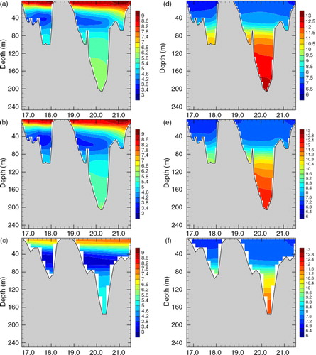
Many similarities are found between the model simulations and the climatology. For example, the strong stratification of temperature and salinity, and the increase of thermocline depth from west to east. However, the 100-yr mean value is not expected to represent the studied period perfectly due to decadal variability. In the eastern Gotland Basin, the deep water is warmer and saltier compared to the western Gotland Basin due to saltwater inflows from Kattegat. Surface layer and deep waters are separated by the cold winter water with minimum temperatures. In general, both temperatures and salinities in FREE are larger than in the climatological data by Janssen et al. (1999). With data assimilation, the differences are reduced. The halocline in FREE is too shallow while with data assimilation the halocline is much closer to climatological data. However, the simulated halocline in REANA is still shallower than the climatological mean halocline, indicating that the studied period 1970–1979 is indeed not representative for the 100-yr mean conditions.

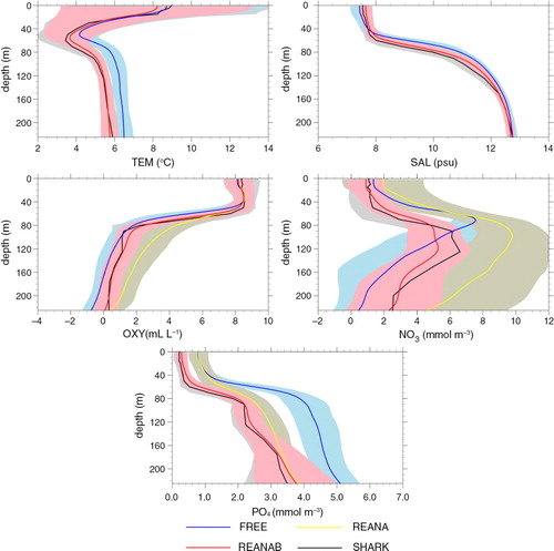
In the following, we discuss differences in mean conditions between the three simulations and observations from SHARK. In Fig. 4, the 10-yr mean (1970–1979) observed and simulated profiles of temperature, salinity and oxygen, nitrate and phosphate concentrations at BY15 (Fig. 1) are shown. The strong vertical salinity gradient in the Gotland Basin is explained by the highly saline inflows from the North Sea, the exceeding evaporation and the large river runoff. In FREE, surface salinity is too low, the halocline separating the saline deep water from the brackish surface layer is too shallow and the temperature of the deep water is too high compared to observations. Further, biases in biogeochemical variables are substantial (Fig. 4). In REANA, the systematic temperature and salinity biases are at all depths considerably reduced and simulated profiles agree very well with observations (Fig. 4). However, the increased ventilation of the Gotland Basin deep water in REANA has large impacts on biogeochemical cycling. Whereas in FREE biogeochemical processes below 160 m depth are carried out on average under anoxic conditions (O₂≤0 mL L⁻¹), in REANA (and observations) these processes occur on average under oxic conditions (O₂>0 mL L⁻¹). As many biogeochemical processes work very differently under oxic and anoxic conditions, deep water nutrient concentrations in the two simulations are consequently very different. Mean nitrate and phosphate concentrations below the halocline differ by up to about 4 and 1.5 mmol m⁻³, respectively.

Fig. 4 Average (1970–1979) vertical profiles for temperature, salinity, oxygen, nitrate and phosphate at BY15 from SHARK (black), FREE (blue), REANA (yellow) and REANAB (red). Shaded areas indicate corresponding standard deviations.

In REANA (and consequently also in REANAB), the overall Baltic Sea RMSDs (Fig. 5) in temperature and salinity are reduced by 38.6% (from 1.66 to 1.02°C) and 25.6% (from 1.21 to 0.90 psu), respectively. Furthermore, the temperature bias has a pronounced seasonal cycle with smallest biases in spring and winter while seasonal variations of the RMSD of salinity are less pronounced. In REANA, the RMSD of oxygen concentration is only slightly reduced compared to FREE (by 5.2%). The RMSD of phosphate concentration is reduced by 30.4% with a gradual improvement with time (Fig. 5) while the RMSD of nitrate concentration is increased by 3.4%.

Fig. 5 Monthly mean root mean square deviation (RMSD) between model results and observations for temperature (a), salinity (b), oxygen (c), phosphate (d) and nitrate (e) in FREE (blue), REANA (yellow) and REANAB (red).

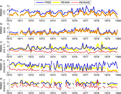
In REANAB the RMSDs of oxygen, phosphate and nitrate concentrations are considerably improved and the RMSD values gradually continue to decrease with time (Fig. 5). Relative to FREE, the overall RMSDs of oxygen, phosphate and nitrate concentrations in REANAB have been reduced by 51.1, 39.8 and 72.1%, respectively. The temporal change of biogeochemical RMSD is most likely due to the adjustment of fluxes from the nutrient pools in the Baltic Sea sediments caused by the imposed changes in physical and biogeochemical conditions in the bottom water. The time scales of changes in the Baltic Sea biogeochemistry are very large, and it takes decades before the sources and sinks are fully balanced to either altered physical conditions or altered nutrient loads (e.g. Meier et al., 2011).

3.2. Time series

Comparing simulated and observed temperatures, we found that in all three simulations the performances in the surface layer are good (Figs. (6–8) and 10). However, in FREE temperatures of the deeper water at BY15 are systematically overestimated (Figs. 7 and 10). Further, mixing of the juvenile freshwater spreading from the gulfs into the Baltic proper seems to be underestimated because the annual cycle in salinity in the surface layer is considerably exaggerated (Fig. 7). The halocline in the Baltic proper is more often ventilated by smaller inflows from the Bornholm Basin than in observations (Fig. 7, see also oxygen concentrations in Fig. 11), and the depth of the halocline is too shallow (Fig. 10). At BY5 temperature biases are even larger than at BY15 but vary in time (Fig. 6) due to the intermittent saltwater inflows from the North Sea through the Danish straits. The FREE simulation underestimates in general the salinity at BY5 (Fig. 6) and shows a deeper halocline than in observations (Fig. 8). There are several simulated saltwater inflows into the bottom layer that are not observed (Fig. 6) because stratification is smaller than observed. At BY15, the salinity of the deep water is overestimated during 1970–1976 and underestimated during 1977–1979 because the large saltwater inflow in spring 1977 is underestimated (Fig. 7). According to observations, this event caused temperatures at 200 m depth to suddenly increase by 1.5°C because of the inflow of warmer water from the North Sea. According to salinity in FREE, the inflow seems to be missing and instead an inflow occurred in 1978 with smaller intensity than the one observed the year before. However, the changes in deep water oxygen concentrations (Fig. 7) indicate that indeed in FREE an inflow in spring 1977 occurred. In REANA, the salt water inflow dynamics are in general considerably improved. The impacts of the inflow in spring 1977 and other smaller inflows are well represented, and reanalysis results for temperature and salinity are almost identical to observations in all layers (Figs. 8 and 10).

Fig. 6 Time series of monthly mean temperature (in °C), salinity (in psu), oxygen (in mL L⁻¹), nitrate (in mmol m⁻³) and phosphate (in mmol m⁻³) in the simulations FREE (blue), REANA (yellow) and REANAB (red) at the depths of 0 m (left panel), 50 m (middle panel) and 80 m (right panel) at BY5 (Bornholm Deep) (55.25°N, 15.98°E) during 1970–1979. Observations are denoted by black dots. For the location see Fig. 1.

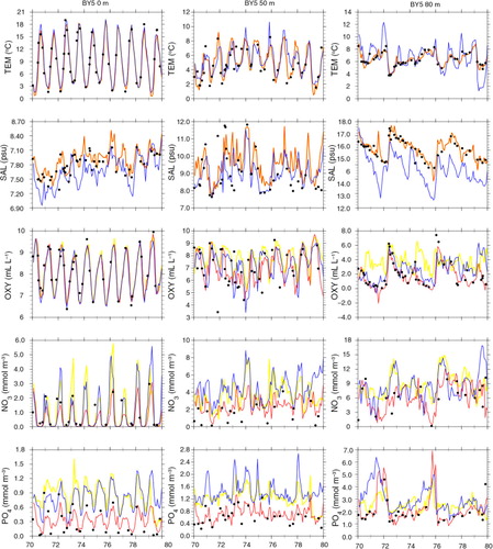
Fig. 7 The same as Fig. 6 but at the depths of 0 m (left panel), 50 m (middle panel) and 200 m (right panel) at BY15 (Gotland Deep) (57.33°N, 20.05°E) during 1970–1979.

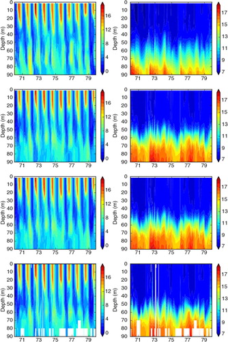
Fig. 8 Isoline depths as function of time for temperature (in °C; left column), salinity (in psu; right column), in the simulations FREE (first row), REANA (second row) and REANAB (third row) and in observations (fourth row) at BY5 (Bornholm Deep) (55.25°N, 15.98°E) during 1970–1979. For the location see Fig. 1.

Similar to temperature, the large seasonal variations in surface oxygen concentrations between summer (~ 6 to 7 mL L⁻¹) and winter (~ 9 to 10 mL L⁻¹) are well simulated in all three experiments (Figs. 6, 7, 9 and 11). In FREE, biases in oxygen concentrations in the deeper layers, especially at BY15, are mainly caused by the above-mentioned shortcomings in saltwater inflow dynamics (Fig. 7). For instance, according to observations, pronounced inflows of water with high oxygen concentrations into the BY5 deep water occur in 1973 and 1975/1976 (Fig. 6). These inflowing waters propagated into the Baltic proper and ventilated the deep water of the eastern Gotland Basin. The events are clearly visible at BY15 in oxygen concentration and temperature but less pronounced in salinity (Fig. 7).

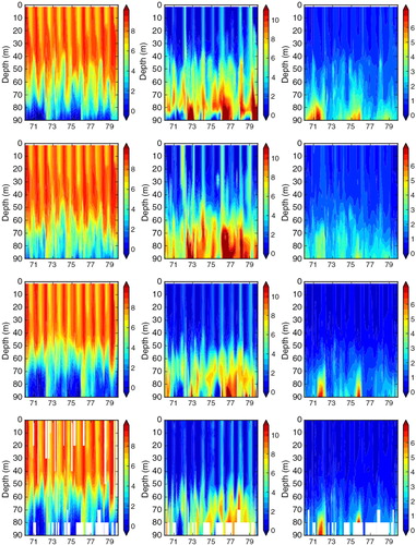
Fig. 9 Isoline depths as function of time for oxygen (in mL L⁻¹; first column), nitrate (in mmol m⁻³; second column) and phosphate (in mmol m⁻³; third column) in the simulations FREE (first row), REANA (second row) and REANAB (third row) and in observations (fourth row) at BY5 (Bornholm Deep) (55.25°N, 15.98°E) during 1970–1979. For the location see Fig. 1.

In REANA oxygen, phosphate and nitrate concentrations are not considerably improved (Table 1). In case of nitrate, the results in REANA are even worse compared to FREE. As a result of the data assimilation in REANA, at all investigated monitoring stations, oxygen concentrations in the deep water are generally increased compared to FREE whereas changes in the surface layer are only small. The higher oxygen concentrations in the deep water in REANA are caused by horizontal inflows of high-saline, oxygen-rich water from Bornholm Basin into the Gotland Basin that are interleaved in particular into the halocline depth (Figs. 10 and 11). As the halocline at BY5 (BY15) is higher (lower) (Fig. 8) compared to FREE (Fig. 10), the horizontal salinity gradients between the subbasins are increased, and consequently inflows are intensified. Compared to observations, oxygen concentrations in REANA are at too high levels, and consequently also nitrate concentrations become too high (Figs. 7 and 11) because of reduced denitrification (anaerobic mineralization of organic matter that transforms nitrate to atmospheric nitrogen N₂) rates under more oxic conditions. In REANAB, however, the assimilation of biogeochemical variables improves the results considerably (Figs. 6, 7 9 and 11).

Fig. 10 The same as Fig. 8, but for BY15 (Gotland Deep) (57.33°N, 20.05°E).

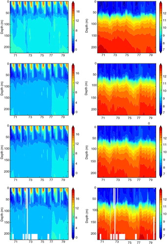
Fig. 11 The same as Fig. 9, but for BY15 (Gotland Deep) (57.33°N, 20.05°E).

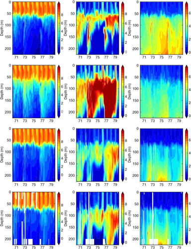
Table 1. Root mean square deviation (RMSD) calculated for the three simulations FREE, REANA and REANAB using temperature, salinity, oxygen, nitrate and phosphate observations from the SHARK data base during the period 1970–1979.

RMSD	Temperature (in °C)	Salinity (in psu)	Oxygen (in mL L^−1)	Nitrate (in mmol m^−3)	Phosphate (in mmol m^−3)
FREE	1.66	1.21	1.53	2.06	1.15
REANA	1.02	0.90	1.45	2.13	0.80
REANAB	1.02	0.90	0.75	1.24	0.32
Reduction REANA	38.6%	25.6%	5.2%	−3.4%	30.4%
Reduction REANAB	38.6%	25.6%	51.0%	39.8%	72.1%

3.3. Impact on biogeochemical cycles

In the following, we illustrate the impact of data assimilation on integrated hypoxic (O₂≤2 mL L⁻¹) and anoxic (O₂≤0 mL L⁻¹) bottom areas (Fig. 12). In general, there is a long-term negative trend during 1970–1979 in the temporal evolution of hypoxic and anoxic bottom areas. In the beginning of the simulation period, there are pronounced maxima in both hypoxic and anoxic bottom areas in all three simulations.

Fig. 12 Time series of the annual mean hypoxic (upper panel) and anoxic (lower panel) areas of the entire Baltic Sea calculated from FREE (blue), REANA (yellow), REANAB (red) and the observations (black).

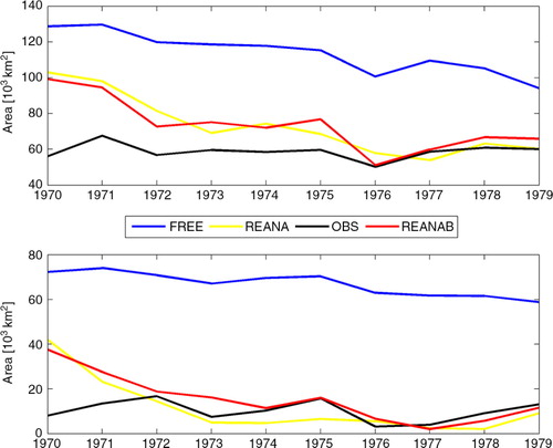
Compared to observations by Hansson et al. (2011), all three simulations overestimate hypoxic and anoxic bottom areas at the beginning of the integration (Fig. 12). Obviously, initial conditions of nutrients in the water column and sediments are not in balance with modelled biogeochemical cycles. Whereas in FREE during the whole integration period both hypoxic and anoxic areas are much larger than observed, the biases in REANA and REANAB become smaller with time. After about 6 yr, simulated hypoxic and anoxic areas are in good agreement with observations. On average, the overall annual mean hypoxic and anoxic bottom areas in the Baltic Sea are reduced by 35.9 and 82.8%, respectively, from 11.4×10⁴ km² and 6.70×10⁴ km² in FREE to 7.3×10⁴ km² and 1.15×10⁴ km² in REANA. In REANAB, the sizes of hypoxic and anoxic bottom areas are similar to REANA, although oxygen concentrations in REANA and REANAB differ considerably (Figs. 9 and 11).

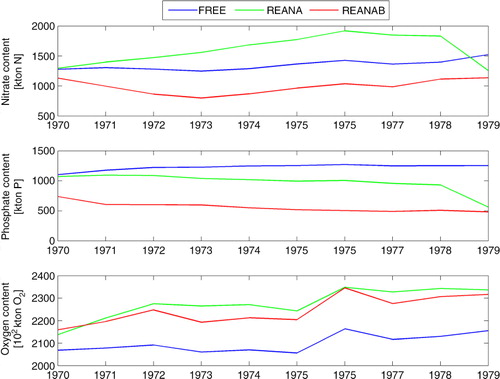
Figure 13 shows the annual mean nitrate, phosphate and oxygen contents averaged for the entire Baltic Sea. The results of the simulations indicate the profound impact of data assimilation on the oxygen and nutrient pools in the water column. In REANA and REANAB, the oxygen and phosphate contents are larger and smaller than in FREE, respectively. The nitrate content in FREE is in between the larger content in REANA and the smaller content in REANAB. In general, inter-annual variations within each simulation are small compared to the large differences between the three simulations. In particular, the phosphate content in REANAB is by more than 50% reduced compared to FREE.

Fig. 13 Time series of the annual mean, volume integrated nitrate (upper panel), phosphate (middle panel) and oxygen (lower panel) contents of the entire Baltic Sea calculated from FREE (blue), REANA (yellow) and REANAB (red).

4. Discussion

Liu et al. (2013) evaluated the performance of the EnOI method from the comparison of assimilated model results with independent temperature and salinity observations that were not used in the assimilation. In this study, we used an independent climatological data set by Janssen et al. (1999) to illustrate the impact of the assimilation on large-scale features like basin-wide thermocline and halocline depths (Section 3.1). The comparison indicated that with data assimilation simulated mean temperature and salinity fields have been improved. However, a comparison of a 10-yr simulation with climatological data that represent 100-yr mean conditions is problematic because the decadal variability in hydrodynamics of the Baltic Sea generated by atmospheric variations like the North Atlantic Oscillation, the Scandinavia pattern (blocking), the East Atlantic/West Russia pattern and the Barents Sea Oscillation is large (Kauker and Meier, 2003; Meier and Kauker, 2003). For instance, the period 1970–1979 was influenced by the large inflow in 1976 that affected both the salinity and the temperature in the deeper parts of the central Baltic. This decade therefore differs from the 100-yr mean conditions with higher than average deep water salinity and temperature in the central Baltic deep water (Fonselius and Valderama, 2003).

Important for biogeochemical cycles are the inflows of salt and oxygen-rich water into the Gotland Basin ventilating the halocline with a maximum in about 100 m depth (e.g. Väli et al., 2013; Eilola et al., 2014). We found that data assimilation of salinity profiles alters large-scale horizontal salinity gradients causing increased ventilation of the deep water in Gotland Basin (Section 3.2). Even when there are no observations from individual inflows, available data assimilation will very likely improve the inflow dynamics because preconditions in stratification and horizontal gradients between Bornholm Basin and Gotland Basin are more realistically simulated.

An important question is how oxygen concentrations in the Gotland Basin deep water are affected by the data assimilation of temperature and salinity profiles. In addition to increased horizontal ventilation, data assimilation also enhances the vertical flux of oxygen because water parcels with low oxygen concentration below the halocline are removed and replaced with water parcels with high oxygen concentration caused by the deepening of the halocline.

Further, there is a feedback to the nutrient cycling in the RCO-SCOBI model due to the oxygen-dependent denitrification rates and phosphorus fluxes between the sediments and the water column (Eilola et al., 2009). Because the phosphorus cycling highly depend on the bottom-water redox conditions, sediments that previously were overlain by anoxic bottom waters are subject to altering phosphorus cycling. The increased oxygen penetration into the sediment impedes the phosphate to diffuse out of the sediments (Mort et al., 2010; Reed et al., 2011). Increased bottom oxygen concentrations and reduced hypoxic and anoxic bottom areas therefore cause reduced phosphorus fluxes from the model sediments, lower phosphate concentrations in the water column, and eventually reduced organic matter production and reduced oxygen consumption due to reduced organic matter decomposition.

At 80 m depth at BY5 (Fig. 6), the oxygen concentrations in REANA relative to FREE are less good compared to observations, but the general increase of oxygen correlates with lowered phosphate concentrations that therefore slightly improved. It is also possible that changing inflow patterns of waters with lower phosphate concentrations from the entrance area in the Danish sounds and the Arkona Basin may have contributed to the lower phosphate concentrations in the deeper parts of the Bornholm Basin. At 200 m depth at BY15 (Fig. 7), the oxygen concentrations in REANA increase too much compared to observations, and the periods with anoxic conditions are completely removed. In this case, it is obvious that the much lower phosphate concentrations in REANA compared to FREE are affected by the higher oxygen concentrations. Furthermore, by looking at phosphate in REANAB at 200 m depth (BY15), we found large state corrections in the form of strong nonlinearities (‘jumps’). These ‘jumps’ are not equally pronounced in the oxygen trajectory of REANAB. Therefore, we conclude that the phosphate concentrations in REANAB are improved by both the information from oxygen and phosphate observations.

All three factors (horizontal and vertical oxygen fluxes and oxygen consumption) may contribute to the differences in oxygen content between the three simulations (Fig. 13). However, the changes in oxygen consumption between FREE and REANA are small because the rate of deep water oxygen decline between the inflows is rather similar in FREE and REANA (Figs. 6 and 7). The decline in REANAB is also fairly similar (indeed somewhat smaller), indicating that in all three cases the oxygen consumption remains unchanged. Because the time scale of the phosphorus cycling is long compared to the integration period in the present study (e.g. Eilola et al., 2011), the difference in surface phosphate concentrations that influence the seasonal primary production remains also rather small between FREE and REANA. As in REANA, simulated oxygen concentrations in the Gotland Basin deep water are overestimated compared to observations due to biased physical conditions. Our experiments may indicate a need of new initial conditions in the sediment and a recalibration of the biogeochemical model. Since the oxygen consumption seems not so much affected by the assimilation, the reason for the too high oxygen concentrations in 200 m depth at BY15 seems to lie in the characteristics of the new deep water that brings large amounts of oxygen into the deeper parts of the Baltic. Possibly, the oxygen consumption is underestimated somewhere in the upstream areas. It is also possible that the problem may become smaller if the model run is longer and the biogeochemistry has more time for an adjustment to the new physical conditions.

In Section 3.3 it is shown that the impact of data assimilation on biogeochemical cycles is considerable. In particular, hypoxic and anoxic bottom areas are reduced in REANA and REANAB compared to FREE, but the differences between REANA and REANAB are relatively small. Hence, the impact of additional assimilation of oxygen observations in REANAB seems to be negligible. The reason might be that organic matter decomposition in the sediments is similar between REANA and REANAB since the initial conditions are identical. The time scales of changes in the pools of nutrients in the sediments of the Baltic Sea are quite long (Eilola et al., 2011) compared to the 10-yr period studied here. In addition, also the pools of organic matter in the water column are initially identical and not directly affected by data assimilation. Hence, the sedimentation of organic matter remains fairly similar for many years between the simulations. Differences in the deep water oxygen consumption between the simulations may therefore be small why the changes in anoxic and hypoxic bottom areas are mainly explained by the changes in the physical conditions like stratification and currents.

5. Conclusions

The main conclusions of this study are:

1. For a 10-yr simulation with a coupled physical-biogeochemical model for the Baltic Sea, very good results are obtained when in situ observations of both physical (temperature and salinity) and biogeochemical (oxygen, phosphate and nitrate) variables are assimilated using the EnOI method. The data assimilation significantly improved the vertical stratification and horizontal gradients, the patterns of inflows and the temporal variations of physical and biogeochemical field variables. The present study shows that the EnOI method works not only for the assimilation of temperature and salinity profile data as shown before but also for the assimilation of available profiles of oxygen, phosphate and nitrate concentration measurements.

2. However, the results of the present study suggest that improved representation of physical processes in a Baltic Sea model obtained by assimilation of temperature and salinity profiles alone does not necessarily improve the results of a coupled biogeochemical model on decadal time scale. This unexpected behaviour is explained by increased oxygen concentrations in the Gotland Basin deep water that are too high compared to observations. As a consequence, nutrient fluxes between water and sediment pools and biogeochemical sources and sinks are significantly modified. The reasons for the elevated oxygen concentrations in the assimilated simulations are increased inflows of oxygen-rich water from the Bornholm Basin and increased vertical oxygen fluxes due to a weaker stratified and deeper halocline in the Baltic proper.

3. We found that hypoxic and anoxic bottom areas are very much affected by changes in halocline depth in accordance with the results by Väli et al. (2013). In general, a deeper halocline causes smaller hypoxic and anoxic bottom areas. These bottom areas do not change much with additional assimilation of biogeochemical observations.

4. To obtain good model results for biogeochemical variables compared to observations when only temperature and salinity observations are assimilated, a recalibration of the biogeochemical model to the modified physics with enhanced horizontal and vertical transports of oxygen would be needed which is out of the scope of the present study. Hence, using the EnOI method all available observations should be used to perform reanalyses of high quality for the Baltic Sea coupled physical-biogeochemical system.

Acknowledgements

We thank two anonymous reviewers for their helpful comments. The research presented in this study is part of the Baltic Earth programme (Earth System Science for the Baltic Sea region, see http://www.baltex-research.eu/balticearth) and was funded by the Swedish Research Council for Environment, Agricultural Sciences and Spatial Planning (FORMAS) within the projects ‘Impact of accelerated future global mean sea level rise on the phosphorus cycle in the Baltic Sea’ (grant no. 214-2009-577) and ‘Impact of changing climate on circulation and biogeochemical cycles of the integrated North Sea and Baltic Sea system’ (grant no. 214-2010-1575) and from Stockholm University's Strategic Marine Environmental Research Funds ‘Baltic Ecosystem Adaptive Management (BEAM)’. Additional support came from the EU-funded project MyOcean2 (Contract FP7-SPACE-20011-1) and the Norden Top-level Research Initiative subprogramme ‘Effect Studies and Adaptation to Climate Change’ through the ‘Nordic Centre for Research on Marine Ecosystems and Resources under Climate Change (NorMER)’.

References

- Almroth-Rosell E. , Eilola K. , Hordoir R. , Meier H. E. M. , Hall P . Transport of fresh and resuspended particulate organic material in the Baltic Sea – a model study. J. Mar. Syst. 2011; 87: 1–12.
- Beckmann A. , Döscher R . A method for improved representation of dens water spreading over topography in geopotential-corrdinate models. J. Phys. Oceanogr. 1997; 27: 581–591.
- Bergström S. , Carlsson B . River runoff to the Baltic Sea: 1950–1990. Ambio. 1994; 23: 280–287.
- Counillon F. , Bertino L . Ensemble Optimal Interpolation: multivariate properties in the Gulf of Mexico. Tellus A. 2009; 61: 296–308.
- Daewel U. , Schrum C . Simulating long-term dynamics of the coupled North Sea and Baltic Sea ecosystem with ECOSMO II: model description and validation. J. Mar. Syst. 2013; 119: 30–49.
- Eilola K. , Almroth-Rosell E. , Dieterich C. , Fransner F. , Höglund A. , co-authors . Modeling nutrient transports and exchanges of nutrients between shallow regions and the open Baltic Sea in present and future climate. Ambio. 2012; 41: 574–585.
- Eilola K. , Almroth-Rosell E. , Meier H. E. M . Impact of saltwater inflows on phosphorus cycling and eutrophication in the Baltic Sea. A 3D model study. Tellus A. 2014; 66 23985, DOI: 10.3402/tellusa.v66.23985.
- Eilola K. , Gustafson B. G. , Kuznetsov I. , Meier H. E. M. , Neumann T. , co-authors . Evaluation of biogeochemical cycles in an ensemble of three state-of-the-art numerical models of the Baltic Sea. J. Mar. Syst. 2011; 88: 267–284.
- Eilola K. , Meier H. E. M. , Almroth E . On the dynamics of oxygen, phosphorus and cyanobacteria in the Baltic Sea; a model study. J. Mar. Syst. 2009; 75: 163–184.
- Evensen G . The Ensemble Kalman filter: theoretical formulation and practical implementation. Ocean Dynam. 2003; 53: 343–367.
- Fonselius S. , Valderrama J . One hundred years of hydrographic measurements in the Baltic Sea. J. Sea Res. 2003; 49: 229–241.
- Fu W . Estimating the volume and salt transports during a major inflow event in the Baltic Sea with the reanalysis of the hydrography based on 3DVAR. J. Geophys. Res. Oceans. 2013; 118: 3103–3113.
- Fu W. , She J. , Dobrynin M . A 20-year reanalysis experiment in the Baltic Sea using three-dimensional variational (3DVAR) method. Ocean Sci. 2012; 8(5): 827–844.
- Fu W. , She J. , Zhuang S . Application of an Ensemble Optimal Interpolation in a North/Baltic Sea model: assimilating temperature and salinity profiles. Ocean Model. 2011; 40: 227–245.
- Gerdes R. , Köberle C. , Willebrand J . The influence of numerical advection schemes on the results of ocean general circulation models. Clim. Dynam. 1991; 5: 211–226.
- Gregg W. W. , Friedrichs M. A. M. , Robinson A. R. , Rose K. A. , Schlitzer R. , co-authors . Skill assessment in ocean biological data assimilation. J. Mar. Syst. 2009; 76: 16–33.
- Hansson M. , Andersson L. , Axe P . Areal extent and volume of anoxia and hypoxia in the Baltic Sea, 1960–2011. Rep. Oceanogr. 2011; 42: 63.
- Hibler W. D . A dynamic thermodynamic sea ice model. J. Phys. Oceanogr. 1979; 9: 817–846.
- Hunke E. C. , Dukowicz J. K . An elastic-viscous-plastic model for sea ice dynamics. J. Phys. Oceanogr. 1997; 27: 1849–1867.
- Janssen F. , Schrum C. , Backhaus J . A climatological data set of temperature and salinity for the Baltic Sea and the North Sea. Ocean Dynam. 1999; 51(Suppl 9): 5–245.
- Kauker F. , Meier H. E. M . Modeling decadal variability of the Baltic Sea: 1. Reconstructing atmospheric surface data for the period 1902–1998. J. Geophys. Res. 2003; 108: 3267.
- Lehmann A. , Myrberg K. , Höflich K . A statistical approach to coastal upwelling in the Baltic Sea based on the analysis of satellite data for 1990–2009. Oceanologia. 2012; 54(3): 369–393.
- Liu Y. , Meier H. E. M. , Axell L . Reanalyzing temperature and salinity on decadal time scales using the ensemble optimal interpolation data assimilation method and a 3-D ocean circulation model of the Baltic Sea. J. Geophys. Res. Oceans. 2013; 118: 5536–5554.
- Liu Y. , Yan C. X . Application of recursive filter to a three dimensional variational ocean data assimilation system. Adv. Atmos. Sci. 2010; 27: 293–302.
- Liu Y. , Zhao Y. L . Assimilation of temperature and salinity using isotropic and anisotropic recursive filters in Tropic Pacific. Acta Oceanol. Sin. 2011; 30: 15–23.
- Liu Y. , Zhu J. , She J. , Zhuang S. Y. , Fu W. W. , co-authors . Assimilating temperature and salinity profile observations using an anisotropic recursive filter in a coastal ocean model. Ocean Model. 2009; 30: 75–87.
- Losa S. N. , Danilov S. , Schröter J. , Janjic T. , Nerger L. , co-authors . Assimilating NOAA SST data into the BSH operational circulation model for the North and Baltic Seas: Part 2. Sensitivity of the forecast's skill to the prior model error statistics. J. Mar. Syst. 2014; 120: 259–270.
- Losa S. N. , Danilov S. , Schröter J. , Nerger L. , Massmann S. , co-authors . Assimilating NOAA SST data into the BSH operational circulation model for the North and Baltic Seas: inference about the data. J. Mar. Syst. 2012; 105–108: 152–162.
- Maar M. , Møller E. F. , Larsen J. , Madsen K. S. , Wan Z. , co-authors . Ecosystem modelling across a salinity gradient from the North Sea to the Baltic Sea. Ecol. Model. 2011; 222(10): 1696–1711.
- Mårtensson S. , Meier H. E. M. , Pemberton P. , Haapala J . Ridged sea ice characteristics in the Arctic from a coupled multicategory sea ice model. J. Geophys. Res. 2012; 117: 00D15.
- Matthäus W. , Franck H . Characteristics of major Baltic inflows – a statistical analysis. Continent. Shelf Res. 1992; 12: 1375–1400.
- Meier H. E. M . On the parameterization of mixing in three-dimensional Baltic Sea models. J. Geophys. Res. 2001; 106: 30997–31016.
- Meier H. E. M . Modeling the pathways and ages of inflowing salt and freshwater in the Baltic Sea, Estuar. Coast. Shelf Sci. 2007; 74: 610–627.
- Meier H. E. M. , Andersson H. C. , Dieterich C. , Eilola K. , Gustafsson B. G. , co-authors . Modeling the combined impact of changing climate and changing socio-economic development on the Baltic Sea environment in an ensemble of transient simulations for 1961–2099. Clim. Dynam. 2012; 39: 2421–2441.
- Meier H. E. M. , Döscher R. , Coward A. C. , Nycander J. , Döös K . RCO – Rossby Centre regional Ocean climate model: Model description (version 1.0) and first results from the hindcast period 1992/93. SMHI Rep. Oceanogr. 1999; 26: 102.
- Meier H. E. M. , Döscher R. , Faxen T . A multiprocessor coupled ice-ocean model for the Baltic Sea: application to the salt inflow. J. Geophys. Res. 2003; 108: 3273.
- Meier H. E. M. , Eilola K. , Almroth E . Climate-related changes in marine ecosystems simulated with a three-dimensional coupled biogeochemical-physical model of the Baltic Sea. Clim. Res. 2011; 48: 31–55.
- Meier H. E. M. , Kauker F . Modeling decadal variability of the Baltic Sea: 2. Role of freshwater inflow and large-scale atmospheric circulation for salinity. J. Geophys. Res. 2003; 108: 3368.
- Mort H. P. , Slomp C. P. , Gustafsson B. G. , Andersen T. J . Phosphorus recycling and burial in Baltic Sea sediments with contrasting redox conditions. Geochim. Cosmochim. Acta. 2010; 74: 1350–1362.
- Neumann T. , Eilola K. , Gustafsson B. , Müller-Karulis B. , Kuznetsov I. , co-authors . Extremes of temperature, oxygen and blooms in the Baltic Sea in a changing climate. Ambio. 2012; 41(6): 574–585.
- Oke P. R. , Schiller A. , Griffin D. A. , Brassington G. B . Ensemble data assimilation for an eddy-resolving ocean model of the Australian Region. Q. J. Roy. Meteorol. Soc. 2005; 131: 3301–3311.
- Omstedt A. , Edman M. , Claremar B. , Frodin P. , Gustafsson E. , co-authors . Future changes in the Baltic Sea acid-base (pH) and oxygen balances. Tellus B. 2012; 64 19586, DOI: 10.3402/tellusb.v64i0.19586.
- Orlanski I . A simple boundary condition for unbounded hyperbolic flows. J. Comput. Phys. 1976; 21: 251–269.
- Pemberton P. , Funkquist L . Data assimilation experiments in the Baltic Sea. 9th HIROMB Scientific Workshop 2831. 2006. SMHI, Gothenburg.
- Reed D. C. , Slomp C. P. , Gustafsson B . Sedimentary phosphorus dynamics and the evolution of bottom-water hypoxia: a coupled benthic–pelagic model of a coastal system. Limnol. Oceanogr. 2011; 56(3): 1075–1092.
- Samuelsson P. , Jones C. G. , Willn U. , Ullerstig A. , Golvik S. , co-authors . The Rossby Centre Regional Climate model RCA3: model description and performance. Tellus A. 2011; 63: 4–23.
- Savchuk O. P. , Gustafsson B. G. , Rodriguez Medina M. , Sokolov A. V. , Wulff F. V . Nutrient Loads to the Baltic Sea. 1970–2006. 2012. Technical Report No. 5. Baltic Nest Institute, Stockholm, Sweden.
- Stevens D. P . The open boundary conditions in the United Kingdom fine-resolution Antarctic model. J. Phys. Oceanogr. 1991; 21: 1494–1499.
- Väli G. , Meier H. E. M. , Elken J . Simulated halocline variability in the Baltic Sea and its impact on hypoxia during 1961–2007. J. Geophys. Res. Oceans. 2013; 118: 6982–7000.
- Zhu J. , Zhou G. Q. , Yan C. X. , You X. B . A three-dimensional variational ocean data assimilation system: scheme and preliminary results. Sci. China (D). 2006; 49(12): 1212–1222.