The sensitivity of characteristics of cyclone activity to identification procedures in tracking algorithms

Abstract

The IMILAST project (‘Intercomparison of Mid-Latitude Storm Diagnostics’) was set up to compare low-level cyclone climatologies derived from a number of objective identification algorithms. This paper is a contribution to that effort where we determine the sensitivity of three key aspects of Northern Hemisphere cyclone behaviour [namely the number of cyclones, their intensity (defined here in terms of the central pressure) and their deepening rates] to specific features in the automatic cyclone identification. The sensitivity is assessed with respect to three such features which may be thought to influence the ultimate climatology produced (namely performance in areas of complicated orography, time of the detection of a cyclone, and the representation of rapidly propagating cyclones). We make use of 13 tracking methods in this analysis. We find that the filtering of cyclones in regions where the topography exceeds 1500 m can significantly change the total number of cyclones detected by a scheme, but has little impact on the cyclone intensity distribution. More dramatically, late identification of cyclones (simulated by the truncation of the first 12 hours of cyclone life cycle) leads to a large reduction in cyclone numbers over the both continents and oceans (up to 80 and 40%, respectively). Finally, the potential splitting of the trajectories at times of the fastest propagation has a negligible climatological effect on geographical distribution of cyclone numbers. Overall, it has been found that the averaged deepening rates and averaged cyclone central pressure are rather insensitive to the specifics of the tracking procedure, being more sensitive to the data set used (as shown in previous studies) and the geographical location of a cyclone.

• cyclone identification
• IMILAST
• cyclone life cycle
• rapidly intensifying cyclones
• synoptic climatology
• reanalysis

1. Introduction

Quantification of cyclone activity in reanalyses, operational analyses and climate model simulations is typically based upon a range of characteristics including cyclone track counts, cyclone centre frequencies, event generation frequency, lifetime, intensity, speed and size. These diagnostics are also valuable when comparing cyclone activity across different data sets (e.g. Hodges et al., 2011; Tilinina et al., 2013) and across different tracking algorithms using a given reference data set (e.g. Neu et al., 2013). However, it is not clear which of these characteristics provide most insight for comparing the results from different schemes and various products. For instance, comparisons of cyclone activity in different reanalyses with a single scheme (Trigo, 2006; Hodges et al., 2011; Tilinina et al., 2013) report a spread in cyclone numbers between the reanalyses, while the differences in the parameters of cyclone life cycle are relatively small. Similarly, comparisons of different numerical algorithms using a reference data set (e.g. Raible et al., 2008; Neu et al., 2013) show a large spread in cyclone counts across the algorithms, while the relative spread in the parameters of cyclone life cycle is much smaller. Consistent with this, Neu et al. (2013), who compared 15 different algorithms applied to the same data set, found that the total number of cyclones varied in different schemes by a factor of 6 (from a low of 2000 to over 12 000 systems per year) with a much smaller range for stronger events. By contrast, they found the relative spread in the parameters of cyclone life cycle (such as life time, intensity and speed of cyclone propagation) was considerably smaller with the largest disparities across methods found for the short-lived, shallow, and slowly moving cyclones, that is, for the transients whose detection is less accurate and more sensitive to the cyclone diagnostic approach applied. Comparison of interannual variability in present and future climate conditions from reanalyses and climate model simulations showed that linear trends, being consistent in sign over the main regions of cyclone activity, may exhibit quite different magnitudes in the outputs from various methods (Neu et al., 2013; Ulbrich et al., 2013).

Neu et al. (2013) concluded that it is difficult to associate scheme-to-scheme differences in cyclone characteristics with a particular feature of the tracking methods. In particular, the results from the vorticity-based schemes and from those using sea level pressure (SLP) do not significantly differ from each other. It has been suggested that the use of vorticity may allow for earlier (compared to SLP) detection of cyclones. However, the vorticity, being proportional to the Laplacian of the SLP field, is much ‘noisier’ than the SLP and requires smoothing prior to cyclone identification (Sinclair, 1994; Hoskins and Hodges, 2002; Hodges et al., 2011). Hence, there are both potential advantages and disadvantages in the choice of field which is used to identify cyclones. It should be pointed out that early detection of cyclones (while bearing in mind the drawbacks associated with false detection) is of central importance in practical matters such as storm development. In a broader sense, missing the genesis phase of cyclones has the potential to distort the climatology of these features. We also mention that likely the largest uncertainties of most schemes occur at the step of building tracks from individual cyclone centres.

Neu et al. (2013) pointed out that the robustness of estimates of cyclone propagation speed (which might become biased in the event of erroneous splitting of continuous tracks or merging different ones) was a concern, since some schemes could not effectively recognise the rapid movement of cyclones. Besides this, there are other disparities between the algorithms associated, for example, with different approaches to treating the cyclones over elevated areas, different requirements on minimum cyclone travel distance, and the various approaches to combining cyclone centres into a track. In other words, despite considerable progress in our understanding of the skills of cyclone tracking methods in Neu et al. (2013), the task of identifying characteristics of tracking algorithms which have a well detectable effect on the characteristics of cyclones (e.g. the use of vorticity and SLP for tracking) has not been fully completed. It was found that no single parameter of the scheme led to a certain difference in cyclone statistics. Given these points, it is important to establish the sensitivity of schemes to these various ‘tuning’ choices. This issue is particularly relevant if we, for example, wish to diagnose how cyclone behaviour has changed over recent decades or may change in the future (as suggested in the CMIP5 models). There is an urgent need to identify which aspects of trends identified with a given algorithm may be associated with the specifics of that algorithm. Conversely, it is of great value to identify which aspects of the response are not so sensitive and, hence, may be regarded as robust across a wide range of schemes.

Here we analyse the sensitivity of cyclone statistics and cyclone life characteristics to different parameters of cyclone tracking algorithms. First, we examine the sensitivity of cyclone climatologies to the filtering cyclone tracks over elevated areas. Filtering of cyclones over elevated topography has traditionally been done because of the potential problem of extrapolating pressure down to sea level. However, the SLP field in such regions may still hold considerable information about synoptic systems in the region. An example of this are storms which penetrate far inland and reach the high elevations over the Antarctic Plateau. A number of case studies have been conducted on these events (e.g. Pook and Cowled, 1999), and their intensity is confirmed by satellite imagery and automatic weather station data. We then analyse the effect of late detection of cyclones on the results and will finally assess schemes’ sensitivity to the impact of potential splitting of tracks at the moment of maximum cyclone migration. These analyses will allow us to identify the cyclone characteristics that are most sensitive to the use of different schemes and, thus, most representative and effective for the comparative assessments.

2. Data and methods

We use cyclone trajectories in the Northern Hemisphere (NH) (coordinates and central pressure) from the IMILAST data base, built using different cyclone tracking algorithms as described in Neu et al. (2013). These tracks were derived from ERA-Interim reanalysis output (Dee et al., 2011) for the period from 1 January 1979 to 31 March 2009, that is, including the ERA-Interim backward extension over the 1979–1988 period compared to the Phase I IMILAST data base (Neu et al., 2013). We use the same scheme numbering as in Neu et al. (2013). Of the 15 algorithms used in Neu et al. (2013), only 12 methods were used here, as some groups did not provide the extension of their dataset (or in a timely manner). Since the publication of the Neu et al. paper, another method (M07) has been added to the database and used in our analysis, making 13 schemes in all. Of these 13 algorithms, five were based on the use of SLP field only and six used vorticity in combination with other fields [e.g. SLP and wind; see details in Neu et al. (2013; Table 1) and for convenience here Table A1 presents the main references for the description of these schemes]. Two methods (M07 and M14) used characteristics of the atmosphere at the 850 hPa level only. The time resolution of all but one of the outputs was 6 hours. In M06, tracking was performed at 12 hourly time steps (at 00 and 12 UTC). The common threshold applied in IMILAST for cyclone life time was 24 hours, which implies at least five 6-hourly synoptic time steps for all schemes and three time steps for M06. Five schemes performed elimination of tracks over regions where the orography exceeded 1000 m (M10, M15, M18) and 1500 m (M02, M20) as a part of the scheme. Except for Section 3, we filtered out cyclones over areas with orography higher than 1500 m by removing track segments over elevated areas. This is similar to Neu et al. (2013); however, instead of 1000 m threshold applied in Neu et al. (2013), we used 1500 m (as in Tilinina et al., 2013).

Table 1. DJF number of tracks that (K) had at least one point over 1500 m in Central Asia (30–55 N, 70–110°E), (K _h ) were observed only over the elevated area, (K ₀) were removed after topographic filtering even though they had some points below 1500 m, (K _z ) remained in the list of tracks after topographic filtering

M06	M09	M12	M16	M22
K	1405	6521	1036	2433	5875
K h	735	3814	425	991	3882
K 0	498	2227	319	1019	1679
K z	179	448	320	441	320

For mapping cyclone characteristics, we used a circular grid with circular cells of a 2° latitude radius (equivalent to approximately 155 000 km²). Parameters of the cyclone life cycle considered here included minimum SLP during the cyclone lifetime (often referred as cyclone intensity), mean and maximum deepening rates, cyclone propagation speed and cyclone lifetime. Following Serreze (1995) and Rudeva and Gulev (2007), all deepening rates were normalised by (sin ϕ _ref /sin ϕ), where ϕ _ref is a reference latitude, taken in this study as 60°. This normalisation accounts for a latitudinal dependence of planetary vorticity [see Rudeva and Gulev (2007), Allen et al. (2010) and Tilinina et al. (2013) for further discussion].

3. The effect of elimination of cyclones over elevated orography

In this section, we examine how elimination of cyclones over elevated areas, where cyclone detection can be somewhat ambiguous, affects the climatology of cyclone activity. As commented above, five algorithms used either a 1000-m or 1500-m threshold to cut out all the systems that were identified over regions where the orography exceeds these heights. In these cases elimination over elevated areas has been done as an integral part of the tracking procedure and, hence, the information about those is not available in the corresponding outputs. For the other eight methods elimination of cyclones over mountainous terrain can be done a posteriori (as in Neu et al., 2013). We removed all the systems found in the areas where the topography exceeded a 1500 m threshold, while the track segments where the topography was lower 1500 m were retained. If the remaining segments lasted less than 24 hours, they were also removed from the outputs. Our analysis is based on SLP-related metrics of cyclone activity (central pressure and deepening rate), often used as a measures of cyclone intensity (Blender et al., 1997; Serreze et al., 1997; Sickmöller et al., 2000; Geng and Sugi, 2001; Gulev et al., 2001; Bauer and Del Genio, 2006; Trigo, 2006; Löptien et al., 2008). Methods M14, M15 and M21 do not provide explicit information on the central pressure and will not be considered for this diagnostic, leaving five schemes (namely M06, M09, M12, M16 and M22) involved with this part of the analysis.

Figure 1 (left column) shows the frequency distribution for minimum cyclone central SLP of all identified cyclones (i.e. for all seasons over our period) over the NH continents in the five schemes after eliminating systems over elevated orography. Histograms are normalised by the total number of tracks. The upper histogram in each panel shows the anomalies of these from the unfiltered data. According to Neu et al. (2013, Fig. 3a and b) the distribution of intensities does not exhibit particularly large variations across the methods. However, variations for the shallow and moderately deep cyclones (1000–1010 hPa) were found to be significant. Figure 1 shows that elimination of the systems over 1500 m produces very little change to the probability distribution of minimum central pressure. Filtering cyclones over elevated orography tends to slightly increase the fraction of shallow cyclones at the expense of moderately deep cyclones. These differences are somewhat more pronounced for the schemes reporting high overall number of tracks (M09 and M22), reaching up to 2%, but even for those schemes the differences are not statistically significant.

Fig. 1 Normalised annual histograms of (left column) the minimum central pressure (hPa) and (right column) the maximum cyclone deepening rate (hPa/6 h) for continental systems over regions where the topographic elevation is less than 1500 m (grey bars) and their deviations from the distribution for all continental cyclones when no elimination is applied (shown in colour). Note the scale difference between the climatological (right) and anomaly (left) axes.

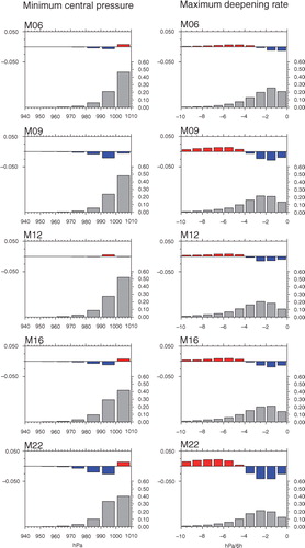
Maximum cyclone deepening rate over continents (Fig. 1, right column) is more sensitive to the elimination of cyclone tracks over elevated areas compared to the cyclone intensity. Elimination of systems over regions where the topography exceeds 1500 m leads to an increase of the fraction of cyclones characterised by moderate to high maximum deepening rates (4–8 hPa/6 h) and a decrease in the fraction of slowly deepening cyclones (here defined as less than 4 hPa/6 h) and this is most pronounced for M09 and M22. This behaviour is seen through the whole year, being most pronounced during winter (figure not shown), when the greatest changes lead to the increase by 6% in the occurrence of slowly deepening systems (from 11 to 17% for<1 hPa/6 h and from 14 to 20% for 1–2 hPa/6 h) observed for M22.

Hence, even though cyclones over highly elevated terrain are, in general, shallower, elimination of these systems produces a minor effect on the averaged characteristics of the cyclone life cycle, especially on the probability distribution of minimum cyclone central pressure. Such a small impact can be explained by propagation of many cyclones generated over the elevated terrain out of those areas. In these cases, cyclones usually reach their minimum central pressure in a lower topography region. On the other hand, the deepening rate often peaks early in a cyclone track and, thus, removal of the first few cyclone points results in a greater effect on the distribution of maximum deepening rates compared to other characteristics of cyclone life cycle.

Despite the small effect associated with the elimination of tracks over elevated terrain on the climatology of cyclone characteristics, one should bear in mind that the effect of mountains is not confined to the immediate location. Large topographic barriers, such as the Rocky Mountains and the Tibetan Plateau (TP), exert significant impact on atmospheric dynamics on the large scale. Lee and Mak (1996) examined the role of the NH orography in the maintenance of storm track areas in winter. They suggested that zonal flow interacting with the orography could reinforce the localised baroclinicity in the western parts of the Pacific and the Atlantic Oceans. Lee et al. (2013) showed that, along with intensification of the upper-level jet and enhancing baroclinicity in the North Pacific Ocean, the TP significantly weakens storm track activity over the TP and East Asia during the cold season. Secondly, the TP amplifies the stationary waves (Siberian high and Aleutian low), which are closely linked to the midlatitude synoptic activity. Broccoli and Manabe (1992) also noted that large-amplitude stationary waves develop owing to the presence of the TP and these waves influence the midlatitude climate. Moreover, Lee et al. (2013), in line with earlier findings of Park et al. (2010), found that the TP suppresses the Pacific storm track during mid-winter. However, here we do not consider this large scale dynamical impact of the elevated terrain on cyclone activity, but rather concentrate on the local effect of frequently applied to the results of cyclone tracking filtering of high terrain areas, as adjusted to the SLP in these areas may be thought of as unreliable.

To explore this in more detail for cyclone characteristics over mountains during winter (December to February, DJF), we selected a region in Central Asia (30–55°N, 70–110°E) stretching from the TP in the south to the Altai Mountains in the north (Fig. 2). The winter season has been chosen as it is the time of enhanced synoptic activity. Table 1 shows the number of cyclone tracks (K) that had at least one point in the region where the topographic height exceeded 1500 m. The climatological (1979–2009) total number of tracks in that region for the cold season varies significantly from about 1000 in M12 to over 6500 tracks in M09 (or from 35 to over 200 tracks per year, respectively). Forty to sixty-five percent of tracks (depending on the method considered) are identified over mountains only, being entirely captured within the elevated area (K _h ). Filtering of tracks over high terrain results in decreasing life time below 24-hour threshold for additional 30–40% of cyclones (K ₀). Note that, despite the wide spread of the K values across the algorithms, the number of tracks that remain after filtering (K _z ) is much more robust (with only M06 being an outlier), and yields about 320 tracks for M12 and M22 and about 440 for M09 and M16. K _z for M06 shows roughly half as many systems as the other methods, which may be due to its lower temporal resolution. (Notice that K _z is not a residual of K, K _h and K ₀ as some of the remaining tracks may be split into two or more tracks (i.e. K≤K _z +K _h +K ₀).)

Fig. 2 DJF maps of characteristics of cyclones in M09 (left) and M12 (right) that had at least one point over the mountains in Central Asia: (a) cyclogenesis, (b) cyclolysis, (c) location of minimum SLP, (d) location of maximum deepening rate, (e) averaged deepening rate for all DJF cyclones (hPa/6 h). Counts in a–d show the number of systems per season in a circle of radius 2 deg. lat. The red line shows the 1500-m topography isoline.

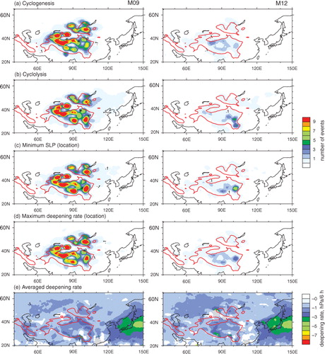
Figure 2 shows climatological maps of cyclone characteristics for the two methods with the highest (M09) and the lowest (M12) number of tracks in the selected area. As implied by Table 1, for the TP region about half of the cyclones are generated, reach their maximum intensity and die within the elevated area. Minimum central pressures are observed in the eastern part of the region, while the maximum deepening rates are often reached in the western part (particularly noticeable for M12), consistent with the cyclone tendency to reach maximum deepening rates at the earlier stages of the development. Maps of the averaged deepening rates for all cyclones (including those identified in the regions where the topography is less than 1500 m) (Fig. 2e) help to detect whether the uncertainties in conversion of surface pressure to SLP produce artefacts in cyclone deepening rates. Moderate deepening rates in the high terrain and at leeward side of mountains for both methods (Fig. 2e) support the finding of Lee et al. (2013) that TP may actually weaken storm track activity over East Asia during the cold season. This is also consistent with our earlier finding that elimination of high terrain cyclones has a very little impact on the climatological distribution of deepening.

In summary, we have demonstrated that elimination of cyclone tracks over elevated areas produces no significant impact on the occurrence histograms of the cyclone central pressure. Maximum deepening rate is slightly more sensitive to the cutoff, especially for the methods which identify a large number of cyclones. Analysis of cyclone characteristics over elevated areas such as the TP and Greenland (results for the latter are not shown here) suggests that, even though orographic filtering may remove a large number of tracks, its effect on the cyclone climatology is quite localised. However, as we already mentioned above, elevated areas are important for maintaining large scale atmospheric dynamics as it has been shown in the previous studies.

4. Impact of the late cyclone detection

We discussed earlier how some detection schemes may have advantages for earlier detection of cyclones. Note that Neu et al. (2013) were not able to identify any scheme-specific aspect (e.g. use of SLP versus low-level vorticity) that was linked to early (or late) detection. To cast light on this issue, we performed a sensitivity study of cyclone life cycle parameters to the moment of identification of a cyclone. For this purpose, we simulated a late identification of cyclones in every scheme by removing the first two points from each track (for M06 only the first point was removed due to the lower time resolution of tracks). This procedure implies the shift of cyclone generation locations and affects the counts of short-lived cyclones, as many of them will fail to meet minimum lifetime criteria and will be removed from the analysis.

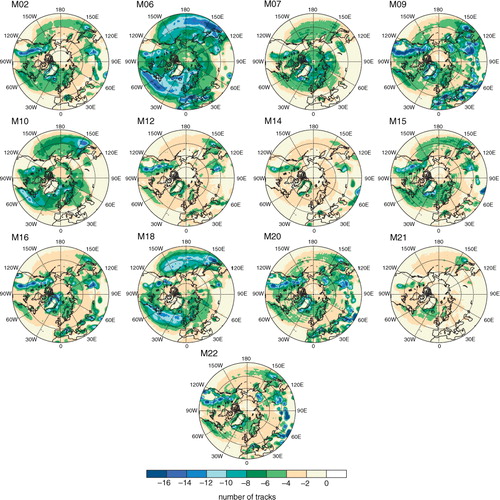
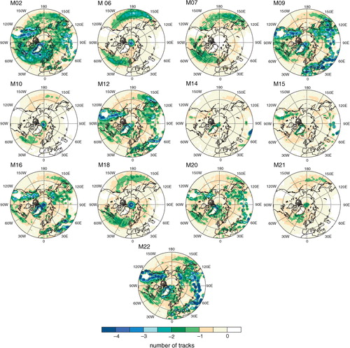
The most noticeable effect is observed for the schemes M06, M10 and M18 in which up to 16 tracks per year per unit area (defined earlier as the area of a circle with a radius of 2 degrees of latitude) were lost over oceans (Fig. 3). For M06, the largest effect is observed in the North Atlantic, North Pacific and over the Mediterranean Sea, while for M10 and M18 these changes are more confined to the North Atlantic and North Pacific storm track areas, with only a minor effect over the Mediterranean Sea. [These marked differences over the Mediterranean Sea between the schemes are perhaps not surprising because that sea poses considerable challenges for cyclone identification (Flocas et al., 2010; Kouroutzoglou et al., 2012). Its location between the subtropics and midlatitudes means it is subject to a range of cyclogenesis processes. In addition, it is a closed basin with complex topography and strong seasonality.] M09 also lost a large number of tracks through this procedure, but this is mainly due to the displacement of cyclone generation areas in the highly elevated regions. It is worth noting that M06 and M18 reported the highest overall number of tracks in the NH (Neu et al., 2013) and that the schemes that lost the highest number of tracks in this experiment (M06, M09, M10, and M18) were all vorticity-based. For the other schemes, the reduction in the number of cyclones in response to the truncation of the starting track segments is less pronounced and tends to be confined to mountains as in M09 (with an exception for M10). The smallest change, which rarely exceeds four tracks per year per unit area, has been found for schemes M12, M14 and M21.

Fig. 3 Annual anomalies in the number of tracks that were reduced by 12 hours from the climatological number of tracks. The counts show the number of tracks per year in a circle of radius 2 deg. lat.

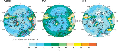
The major relative decrease in the number of cyclones due to removal of the first 12 hours of the life cycle (i.e. absolute difference normalised by the climatological number of tracks) is found over the southern flank of the major storm track areas with the differences over the core of storm tracks over the oceans being minor (Fig. 4). The strongest relative decrease in the number of tracks over mountain regions (up to 90%) can be explained by the displacement of the storm generation locations from the ‘true’ ones. On average, the reduction in the number of tracks is about 10–20% and is double this in the main storm track areas. Again M06 stands out in these plots with 30–40% reduction observed over large areas, that is likely due to the lower temporal resolution of the tracks in this method. Relative changes in the number of cyclones show that the reduction in the number of short-lived systems due to elimination of tracks, that lasted less than five time steps, is not confined to the main storm track areas, as one may have concluded from Fig. 3, but is quite evenly distributed over the hemisphere. This implies that earlier identification of cyclones by the vorticity-based methods does not significantly change the pattern of cyclone activity and that comparison of cyclone climatologies for methods based on different variables (vorticity vs. SLP) would not show significant differences.

Fig. 4 (Left panel) Annual relative anomalies in the number of cyclones averaged across the schemes and (middle and right panel) two most contrasting examples after the first 12 hours of each track were removed. The counts show the number of tracks per year in a circle of radius 2 deg. lat. The red contour lines in the left panel show the standard deviation.

Bearing in mind that the beginning of a cyclone's life cycle is frequently characterised by rapid intensification (Rudeva and Gulev, 2011), it is informative to assess the extent to which other cyclone properties are influenced by the elimination of the first 12 hours of the cyclone life cycle. We found that 40–50% of all cyclones, depending on a method, reach their maximum deepening rates within the first 12 hours of their life cycle and, hence, the occurrence histograms of cyclone characteristics may also undergo changes when the starting points of cyclone tracks are removed. Although the impact on the lifetime distribution is obvious (not shown), it is interesting that the averaged life time does not change much after the cutoff and, depending on a method, may either decrease (by a maximum of 5% for M02 and M18) or increase (by a maximum of 7% for M21) (Table 2). As short-lived cyclones are typically less intense, the removal of the first segment of a track would reduce the percentage of weak systems (not shown); however, it is less straightforward how the deepening rates will behave in this sensitivity analysis. Figure 5 shows the impact of the truncation of the first 12-hour segments of the tracks in the distribution of maximum deepening rate. The upper histogram in each panel shows the anomalies of the distribution for the truncated tracks from the climatological distribution. Histograms are normalised by the total number of tracks, that is, display relative frequencies. The largest impact is seen for schemes M02, M06, M12 and M18. Interestingly, for M06 (the scheme, for which the highest number of tracks was removed), the fraction of slowly intensifying systems (<1 hPa/6 h) decreases, but increases in all other schemes. This reduction for M06 may be explained by removing short-lived cyclones of a small intensity, which rarely achieve rapid deepening rates. On the other hand, an increase in the relative number of slowly intensifying cyclones in the other schemes (M02, M12 and M18) can be explained by the cutoff of the starting track segments associated with the fastest deepening, so that some tracks that had been originally attributed to a moderate or fast deepening category would become slowly deepening systems after the cutoff of the starting segments. The latter effect is also observed for M09, M20 and M22 with the largest increase in the occurrence of cyclones deepening at the maximum rate of 1–3 hPa/6 h. Overall, occurrence anomalies for maximum deepening rates, implied by the cutoff of the initial track segments, tend to be higher for the schemes with the higher overall number of tracks. However, the sign of deviations and, therefore, the possible cause of differences in the shape of probability distributions cannot be directly associated with the parameter used for cyclone identification (vorticity, SLP or Z850).

Fig. 5 Normalised annual climatological histograms of the maximum cyclone deepening rate (hPa/6 h) (; grey bars) along with the magnitudes of deviations of histograms implied by the truncation of the first 12 hours of cyclone tracks () from the original ones ( ; colour bars). = – .

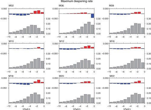
Table 2. Average duration of tracks before (LT) and after (LT12) the removal of the first 12 hours of each track (days) and difference between them (absolute, D _LT , and normalised by LT, R _LT )

LT	LT12	DLT	RLT (%)
M02	3.63	3.45	−0.19	−5
M06	2.16	2.25	0.09	4
M07	2.37	2.42	0.05	2
M09	2.66	2.83	0.16	6
M10	2.52	2.57	0.05	2
M12	4.07	3.98	−0.09	−2
M14	3.66	3.73	0.07	2
M15	2.82	2.86	0.04	2
M16	2.93	3.06	0.14	5
M18	3.54	3.35	−0.19	−5
M20	2.71	2.85	0.14	5
M21	2.48	2.65	0.18	7
M22	2.65	2.79	0.14	5

Following on the discussion on maximum deepening rates, we calculated the number of rapidly intensifying cyclones (RICs) in each method, that is, cyclones that reached a deepening rate of ≥6 hPa per 6 hours at least once during their lifetime. We note here that this approach differs from the more often used one, in which RICs are defined as systems deepening faster than 1 Bergeron (24 hPa per 24 hours) as implied by Sanders and Gyakum (1980) and Lackmann et al. (1996). [More extensive discussion on these definitions can be found in Lim and Simmonds (2002), Allen et al. (2010) and Tilinina et al. (2013). Also note that the threshold of 6 hPa/6 h did not have to be corrected to the 60° latitude as in Sanders and Gyakum (1980) because all cyclone deepening rates were normalised as described in Section 2.] The proportion of deepening cyclones that are RICs varies from 11 to 25% across the schemes with about one third reaching the rate of 6 hPa/6 h during the first 12 hours only. Thus, they will not be classified as RICs in the case of our synthetic late cyclone identification. Nearly half of RICs demonstrate a rapid intensification at a later stage (i.e. at least 12 hours after their identification) and, thus, will fall into the RIC category (Table 3). Interestingly, even though the percentage of RICs in the total number of cyclones varies across the methods by a factor of about two, the ratio between the RICs showing earlier and later intensification during their life time is quite robust in the various methods.

Table 3. Number of RICs per scheme per 30-year period

M02	M06	M09	M10	M12	M16	M18	M20	M22
RIC	18 781 (24.7)	10 127 (10.7)	14 370 (14.1)	8495 (16.7)	14 563 (21.5)	11 959 (18.5)	10 573 (14.9)	19 142 (20.5)	10 295 (17.0)
RIC1	6405 (8.4)	2716 (2.9)	5667 (5.6)	2716 (5.4)	4869 (7.2)	3865 (6.0)	3333 (4.7)	6611 (7.1)	3872 (6.4)
RIC2	3949 (5.2)	1779 (1.9)	2640 (2.61)	2740 (5.4)	3053 (4.5)	2276 (3.5)	1405 (2.0)	3632 (3.9)	2395 (3.9)
RIC3	8427 (11.1)	5632 (6.0)	6063 (6.0)	3039 (6.0)	6641 (9.8)	5818 (9.0)	5835 (8.2)	8899 (9.5)	4028 (6.6)

RIC₁ – cyclones that were rapidly intensifying only within the first 12 hours; RIC₂ – cyclones that were rapidly intensifying within the first 12 hours and at least once later; RIC₃ – RIC, that did not show rapid intensification within the first 12 hours of their development. Absolute numbers are shown in regular font and italic is used to show the relative values normalised by total number of tracks.

5. Effect of splitting of tracks

Besides the uncertainty of identification of the cyclone generation moment, which may vary from method to method, another source of uncertainty is associated with the ‘splitting’ of tracks. The term splitting usually implies splitting of multi-centre cyclones that occurs frequently for the intense systems (Hanley and Caballero, 2012). Unfortunately, this process is poorly accounted for in the modern cyclone tracking algorithms; it is represented in only three out of 15 schemes evaluated by Neu et al. (2013) (M13, M14, M21). All other algorithms treat cyclones as a single-centered object, which makes tracking easier, although partly at the expense of realistic representation of cyclone structure and development.

However, in some cases splitting of a cyclone track by a numerical scheme may also occur in a single-centre system as a result of fast cyclone propagation. Figure 6 shows that mean speed of cyclone propagation ranges from 20 to 40 km/h for 50% of cyclones, while some storms may reach a maximum speed in excess of 100 km/h. There was a concern expressed in Neu et al. (2013) that some algorithms might not be capable of tracking systems during the stage of their fastest propagation that results in either splitting trajectories or termination of track at the point of the fastest propagation. Analysis of cyclone propagation velocities (Fig. 7a) shows, however, that in some cases cyclones may reach unrealistically high speeds of 250 km/h and more (in M12 and M16, the number of such tracks per year is about 31 and 67, respectively). As suggested by Fig. 7b in some cases such high speeds have been observed over the elevated areas and, thus, might be filtered applying orographic threshold. However, our test showed that filtering of elevated areas reduces the number extremely fast moving cyclones (≥250 km/h) by less than 10%. At the same time, very fast propagation of cyclones (≥170 km/h) has been identified even over the oceanic storm tracks and in the Mediterranean. Such high speeds might be potentially diagnosed due to the erroneous merging of two independent cyclone trajectories into one track. However, it is difficult to set a specific threshold on the maximum cyclone speed, as it will largely depend on the background field in which the cyclone propagation takes place. Nevertheless, to address the problem of a potentially spurious fast propagation, we will explore here the extent to which splitting of tracks at the time of the fastest cyclone migration affects statistics of cyclone characteristics. We considered only cyclones exhibiting at least once the peak velocity higher than 100 km/h. For these cyclones, we simulated splitting of tracks at the moments of peak velocity by cutting them into two shorter tracks. As one would expect, due to imposition of a minimum lifetime threshold, this procedure would result in removal of some short tracks that have been formed after the simulation of splitting (as in the case with simulation of the late identification of cyclones). We note here that we only applied a single split of the trajectories at the moment of their fastest propagation, but did not set up an overall threshold on the cyclone speed; that is, in the remaining segments of the tracks, speed may still be over 100 km/h. From 56 to 96% of tracks (depending on the scheme) never reach speed higher than 100 km/h (Table 4) and, hence, remain unchanged after the application of the splitting simulator (R). For some cyclones, both track segments remain in the dataset after splitting simulation. The percentage of such tracks ranges from 0.8% for M06 to 17.5% for M12. In many cases (up to 22% for M02 and M12), simulation of splitting resulted in removal of one of the two segments of a cyclone, while from 0.7 to 7.2% of tracks disappeared completely as both new tracks were too short to pass the life time threshold.

Fig. 6 Distribution of (a) average and (b) maximum propagation speed of a cyclone centre.

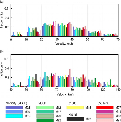
Fig. 7 (a) Tail of annual distribution of maximum propagation speed of a cyclone centre for tracks prior to orographic filtering and (b) spatial distribution of the number of tracking schemes that demonstrate a cyclone speed of 170 km/h and more. The counts show the number of tracking schemes in a circle of radius 2 deg. lat.

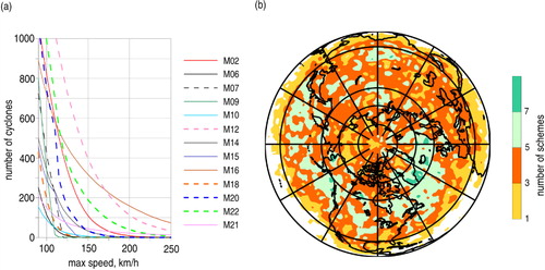
Table 4. Number of tracks (N) per scheme before splitting and the number of tracks that remained unchanged (R)

M02	M06	M07	M09	M10	M12	M14	M15	M16	M18	M20	M21	M22
N	84 110	130 188	53 408	125 680	62 928	78 548	46 873	73 723	79 092	85 564	118 039	43 682	72 436
R	55 333 (65.8)	124 754 (95.8)	45 521 (85.2)	98 507 (78.4)	58 796 (93.4)	43 670 (55.6)	38 361 (81.8)	64 900 (88.0)	59 283 (75.0)	77 361 (90.4)	98 164 (83.2)	37 783 (86.5)	45 988 (63.5)
N->2	9015 (10.7)	1064 (0.8)	1876 (3.5)	5596 (4.4)	1377 (2.2)	13 770 (17.5)	2872 (6.1)	1994 (2.7)	4674 (5.9)	2740 (3.2)	4316 (3.7)	1529 (3.5)	6516 (9.0)
N->1	18 247 (21.7)	3018 (2.3)	4850 (9.1)	15 881 (12.6)	2292 (3.6)	17 093 (21.8)	4509 (9.6)	5625 (7.6)	11 772 (14.9)	4507 (5.3)	12 584 (10.7)	3524 (8.3)	14 723 (20.3)
N->0	1515 (1.8)	1352 (1.0)	1161 (2.2)	5696 (4.5)	463 (0.7)	4015 (5.1)	1131 (2.4)	1204 (1.6)	3363 (4.3)	956 (1.1)	2975 (2.5)	746 (1.7)	5209 (7.2)

Tracks that were split into two tracks (N→2); were split, but only one part of the track remained in the dataset (N→1) or tracks that disappeared completely after splitting (N→0). Absolute numbers are shown in regular font, and italic is used to show the relative values normalised by N.

Figure 8 shows a reduction in the number of tracks after applying the simulation of splitting for the fast moving cyclones. The most sensitive to this procedure are schemes M02, M09, M12 and M22. Of these, M02 loses tracks both at the border of mountainous regions and over oceanic storm tracks, while others are most sensitive to the track splitting in the areas of complicated topography (more than four lost tracks per unit area). M06 and M07 lose tracks mainly over the oceanic storm track (up to three tracks per unit area). Considerable reduction of the number of tracks over the areas of complicated orography is mostly associated with the truncation of the starting points of the trajectories, when cyclone propagation speed is high; on the other hand, decrease in the number of systems over oceanic storm tracks is caused by a reduction of the number of relatively short-lived cyclones. However, if splitting of a track occurs at the mature stage of the cyclone development, there is little impact on the climatology of the number of cyclones, although it may affect some other characteristics of cyclone activity, such as track-averaged speed, areas of generation, etc. Remarkably, the histogram of maximum speed (Fig. 6b) shows a large spread across the methods. Thus, methods M06 and M10 indicate the highest number of tracks that only reach 40–60 km/h, while methods M07 and M18 have a relatively large number of tracks with speeds of 100 km/h. For the M22 algorithm, more than 17% of cyclones reach a speed of more than 120 km/h. Occurrence histograms of maximum deepening (not shown) demonstrate that splitting of tracks leads to an increase in the relative number of slowly deepening cyclones (<3–4 hPa/6 h) and to a decrease of the fraction of cyclones with higher deepening rates. This might happen due to the truncation of the first part of the tracks when cyclones demonstrate their maximum deepening rate.

Fig. 8 Annual anomalies of the number of tracks that were split at their maximum propagation time step from the climatological number of tracks. The counts show the number of tracks per year in a circle of 2 deg. lat.

6. Discussion: robustness of cyclone characteristics

As commented in the Introduction, for obtaining an overall diagnosis of cyclone systems with state-of-the-art numerical algorithms, it is important that we are able to identify which parameters of cyclone activity are more and which are less sensitive to the choice of tracking algorithms (and, thus, which are robust outputs of tracking methods). Up till now, our analysis has been focused on quantifying the effects of potential shortcomings of the tracking algorithms on various characteristics of cyclone activity, such as cyclone numbers, intensity and deepening rates. We now assess the robustness of cyclone life cycle characteristics with respect to the potential drawbacks. Figure 9a shows maps of the maximum cyclone deepening rates in DJF averaged across the nine methods. The averaged maximum deepening rates reach the highest values over the oceans (up to 7 hPa/6 h); however, all over the NH the values demonstrate a large spread across the algorithms. Even over oceanic storm track areas, where the standard deviation (STD) of maximum deepening rates reaches its minimum, maximum deepening rates vary considerably from 4 to 7 hPa/6 h for M06 to more than 10 hPa/6 h for M02. Recall that M02 and M06 schemes diagnose the highest overall number of cyclones in DJF (Fig. 11a), while M06 shows the minimum number of intense cyclones (that reach 970 hPa) and M02 reports a much higher number of intense and moderate systems than any other method.

Fig. 9 DJF maps of (a) maximum deepening rate (hPa/6 h), (b) average deepening rate (hPa/6 h) and (c) average central pressure of cyclones (hPa). The left panels show average between the methods and middle and right panels show the two most contrasting schemes. The red contour lines show the STD.

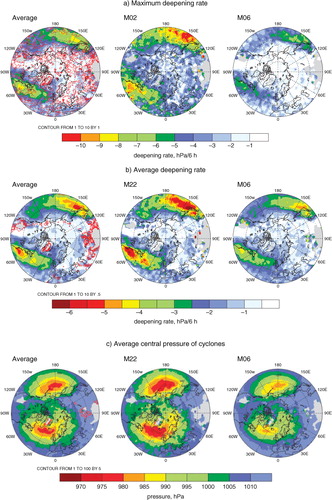
In contrast to the maximum deepening rate, analysis of mean deepening rates reveals much more similarity between the methods (Fig. 9b). On average in DJF, mean deepening rates reach 6 hPa/6 h over Atlantic and Pacific (implying higher occurrence of RICs over the oceanic storm tracks), being much weaker (only up to 3 hPa/6 h) over the continents. M06 shows slightly lower values of deepening compared to the other methods and also exhibits lower STD compared to the averaged maximum deepening rates, shown in Fig. 9a (except for the highly elevated areas, where the results should be treated with caution; see also Section 3 for a discussion). Thus, the average deepening rate is less sensitive to the algorithm setting and reflects more the characteristic of the dataset used (Tilinina et al., 2013). Quite naturally, much smaller mean deepening rates (up to 1.5 hPa/6 h over the continents and 2 hPa/6 h over the oceans) and less agreement between algorithms were found during the warm season (not shown). Another parameter which is relatively insensitive to specific features of the tracking algorithms is the geographical distribution of averaged central pressure of cyclones (Fig. 9c). In all the algorithms, the averaged central pressure over the oceanic storm track areas in DJF reaches 970 hPa and a minimum of 990 hPa over the continents, except for M06 for which the central pressure is typically 5–10 hPa higher. One can see that the minima of the local cyclone central pressure over the midlatitude oceanic storm track areas are well co-located in different algorithms, despite of quite large disparities in the number of cyclones (see Neu et al., 2013; Fig. 1).

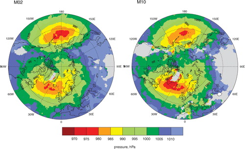
In our analysis, it is also useful to highlight the difference between the results of two algorithms which are based on the same core code but use different parameter settings, namely, M02 and M10. Method M02 shows a higher number of cyclones, in particular in the Mediterranean region, compared to M10 (Neu et al., 2013; Fig. 1). Given generally close agreement between the climatologies for deep systems, we hypothesise that the difference comes from the contribution from weaker and consequently smaller (Simmonds, 2000; Rudeva and Gulev, 2007) cyclones, which are harder to detect. This might explain the higher local cyclone centre pressure in M02 in the Atlantic and Mediterranean (Fig. 10); however, it is difficult to explain why in the Pacific M02 shows lower cyclone local central pressure compared to M10. In summer (not shown), the averaged local cyclone central pressure rarely drops below 995 hPa and is less consistent across the methods over both over oceans and continents, showing larger geographical discrepancies. Thus, in different cyclone tracking methods, the mean local central pressure may vary within 5–10 hPa depending on the particular parameter settings.

Fig. 10 DJF map of average central pressure of cyclones (hPa) for M02 and M10.

Our analysis has shown that cyclone tracking methods that produce a large number of cyclones are the most sensitive to different thresholds and parameter settings. Figure 11a and b shows the number of cyclones identified by different methods depending on cyclone intensity. The cumulative histograms in the figure are built using 10-hPa wide bins, and the dots, representing the cumulative number of tracks, are placed in the centre of the bins. In DJF all the methods except for M02 agree well in the range of central pressure below 980 hPa. In JJA, this range increases to about 990 hPa. Table 5 shows the percentages of the 200 most intense cyclones in the total cyclone count along with their central pressure for different methods. These 200 most intense cyclones constitute per season 19–44% and 17–39% of all cyclones in DJF and JJA, respectively. We note a slight mismatch between the estimates given in Table 5 and those that might be derived from Fig. 11a and b. This is due to the use of 10 hPa bins in Fig. 11a and b, while in Table 5 the percentages and corresponding SLP minima were estimated explicitly. Generally, for the 200 most intense cyclones per season, all schemes agree relatively well in both winter and summer. The average intensity of the 200th most intense cyclone per season ranges between 985 hPa and 992 hPa in DJF (with an exception for M02 for which this value drops to 980 hPa) and between 994 and 998 hPa in JJA. In Fig. 11c and d, we show winter and summer climatologies of cyclone numbers averaged over the nine schemes from the IMILAST ensemble based on these 200 most intense systems along with STD estimates. In winter, the maximum is located over the oceanic storm track area, and variability across the methods of the number of tracks of most intense cyclones is typically less than 30% of the mean. In summer, a significant number of extreme cyclones propagate to the north-east of North America, in the north of Siberia and in the Arctic with a remarkably low variability across the methods (STD being less than 20–25% of the mean). Note that even though 1500 m threshold has been applied in the selection procedure, there is still some remaining noise in the areas close to the mountains in Asia in the summer plot (it may be associated with the pressure adjustment over elevated areas that are below 1500 m). Therefore, in the NH there are about 800–1000 cyclones per year which can be reliably identified by any method and deserve high confidence, but other cyclones, that are identified on top of that, are rather sensitive to the specific techniques applied.

Fig. 11 (a) DJF and (b) JJA cumulative distribution for the number of tracks per season as a function of cyclone intensity (minimal central pressure). The plots are built using 10-hPa wide bins, and the dots are placed in the centre of the bins. (c) DJF and (d) JJA number of 200 most intense cyclone tracks averaged across the algorithms per each season (in colour). The counts show the number of tracks per year in a circle of 2 deg. lat. Red contour lines show STD.

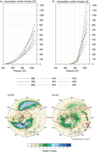
Table 5. The percentage of the total number of cyclones per season (DJF and JJA) which fall into the ‘200 most intense cyclones’ category (P ₂₀₀) and the average SLP (hPa) in the centre of the 200th most intense cyclone in a season at the moment of its maximum intensity (SLP ₂₀₀)

DJF		JJA
P 200	SLP 200	P 200	SLP 200
M02	27	980	30	996
M06	19	985	17	997
M09	25	989	14	994
M10	37	986	39	998
M12	44	992	23	995
M16	36	989	25	994
M18	24	986	32	998
M20	24	989	17	994
M22	39	990	26	994

Table A1. Code numbers for the tracking methods used in this study, the main references for method descriptions and figures in which each method was used

Main references for method description	Figures
Code	1	2	3	4	5	6	7	8	9	10	11
M02	1991), Pinto et al. (2005)	✓	✓	✓	✓	✓	✓	✓	✓	✓
M06	1997), Hewson and Titley (2010)	✓	✓	✓	✓	✓	✓	✓	✓	✓
M07	Flaounas et al. (2014)	✓	✓	✓	✓
M09	1995), Wang et al. (2006)	✓	✓	✓	✓	✓	✓	✓	✓	✓	✓
M10	1991), Simmonds et al. (2003)	✓	✓	✓	✓	✓	✓	✓	✓	✓
M12	2002), Rudeva and Gulev (2007)	✓	✓	✓	✓	✓	✓	✓	✓	✓	✓
M14	Kew et al. (2010)	✓	✓	✓	✓
M15	1997), Raible et al. (2008)	✓	✓	✓	✓
M16	2002)	✓	✓	✓	✓	✓	✓	✓	✓	✓
M18	1994, 1997)	✓	✓	✓	✓	✓	✓	✓	✓
M20	2006)	✓	✓	✓	✓	✓	✓	✓	✓
M21	2009)	✓	✓	✓	✓
M22	2005), Akperov et al. (2007)	✓	✓	✓	✓	✓	✓	✓	✓	✓

7. Summary and outlook

We have analysed the sensitivity of different characteristics of cyclone activity in the NH for the assessment of skills of tracking algorithms using IMILAST ensemble of cyclone trajectories obtained using 13 different detection and tracking methods with the intention of shedding more light onto, and to add more dimensions to, the comparative assessment by Neu et al. (2013). We conducted several sensitivity tests targeting most problematic aspects of cyclone tracking. A particular focus was on the impact of elimination of tracks over elevated orography, late cyclone detection, and splitting of cyclone tracks at the moments of the fastest propagation onto different characteristics of cyclone activity (cyclone counts, probability distributions of the parameters of cyclone life cycle). In accord with the comments of Neu et al. (2013), we remark that we have also found it difficult to associate specific features of the cyclone tracking schemes with a particular behaviour of algorithms in the sensitivity experiments. Instead, we aimed to show what parameters of cyclone activity are the most sensitive to the differences in the approaches used to identify and track cyclones.

To the extent that it is possible to derive compelling inferences from 13-member ensemble, using the concept of a posteriori assessment of potential drawbacks in tracking algorithms, the following major conclusions can be drawn:

1. Filtering of cyclones over elevated terrain (in excess of 1500 m) has no significant impact on the cyclone intensity distribution; however, it may seriously affect the other characteristics of cyclone activity and parameters of cyclone life cycle such as number of cyclones and deepening rates;

2. Late identification of cyclones (simulated by the truncation of the first 12 hours of cyclone life cycle) leads to a large reduction in the number of cyclones. This effect is more pronounced over the continents, particularly in the lee of the mountains, where cyclone reduction may reach 50–80%. Over the oceanic storm track areas about 20–40% of tracks might be lost due to late cyclone detection;

3. Potential splitting of the trajectories at the moment of fast propagation has a negligible climatological effect on geographical distribution of cyclone numbers. It should be noted that very fast propagation is frequently observed in the areas with complicated orography and might often be masked out by the procedure of filtering elevated areas;

4. Averaged local deepening rates are rather insensitive to the specifics of the tracking procedures and likely depend more on the data used rather than the method. Another robust characteristic, which is insensitive to the potential drawbacks of numerical algorithms at least in winter, is the local cyclone centre pressure. At the same time in summer, extreme values of either of these parameters (local deepening rate or cyclone intensity) show considerably less consistency across the methods;

5. All cyclone tracking methods agree well on the identification and characteristics of the 200 deepest cyclones per season (19–44% of the total number of cyclones in winter and 17–39% in summer). In winter these systems are confined by the oceanic storm track areas, whereas in summer they are primarily observed in the northern midlatitudes and polar regions.

In the future, there is a number of directions for a potential extension of our study. First, our results imply the need for the extensive numerical experimentation with different tracking algorithms in order to provide more comprehensive knowledge about potential shortcomings of algorithms which are presently poorly or not at all documented. For now, in the first stage of IMILAST (Neu et al., 2013), most algorithms were assessed, holding the core of codes frozen. We believe that our sensitivity analysis will be a first step in encouraging tracking code developers to target refinements of particular aspects of their numerical algorithms. In particular, while some tracking schemes may have limits on the maximum propagation speed, two methods (M12 and M16) have shown cyclone speeds well beyond physically realistic values and, possibly, their codes need some revision in relation to this question. Secondly, our approach can be potentially applied to compare sensitivity of selected tracking methods using various reanalysis data to better understand the differences in cyclone activity in different reanalyses (Hodges et al., 2011; Tilinina et al., 2013). It has been shown that cyclone characteristics derived from modern era reanalyses generally agree well with each other; however, the total counts of cyclone tracks are significantly different between datasets and the higher number of deep cyclones was found in MERRA. At the same time both here and in Neu et al. (2013), we demonstrated that cyclone counts vary significantly depending on the identification method applied. Thus, it will be of interest to compare a spread in cyclone climatologies by using a few datasets and tracking methods to find out which disparities in cyclone activity are the most robust and which characteristics hold through various methods and data.

Acknowledgements

We thank Swiss Re for sponsoring the IMILAST project and ECMWF for providing the ERA-Interim reanalysis. Parts of this research were made possible by a grant from the Australian Research Council. We also benefited from the grant No. 14.B25.31.0026 by the Russian Ministry for Education and Science for establishing excellence at Russian Universities and research centres as well as from the contract no. 14.607.21.0023 with the Russian Ministry for Education and Science.

9. Appendix

In Table A1, we present the main references for the design and description of the 13 cyclone identification and tracking methods used in this study.

References

- Akperov M. G. , Bardin M. Y. , Volodin E. M. , Golitsyn G. S. , Mokhov I. I . Probability distributions for cyclones and anticyclones from the NCEP/NCAR reanalysis data and the INM RAS climate model. Izvest. Atmos. Ocean. Phys. 2007; 43: 705–712.
- Allen J. T. , Pezza A. B. , Black M. T . Explosive cyclogenesis: a global climatology comparing multiple reanalyses. J. Clim. 2010; 23: 6468–6484.
- Bardin M. Y. , Polonsky A. B . North Atlantic Oscillation and synoptic variability in the European-Atlantic region in winter. Izvest. Atmos. Ocean. Phys. 2005; 41: 127–136.
- Bauer M. , Del Genio A. D . Composite analysis of winter cyclones in a GCM: influence on climatological humidity. J. Clim. 2006; 19: 1652–1672.
- Blender R. , Fraedrich K. , Lunkeit F . Identification of cyclone track regimes in the North Atlantic. Q. J. Roy. Meteorol. Soc. 1997; 123: 727–741.
- Broccoli A. J. , Manabe S . The effects of orography on midlatitude Northern Hemisphere dry climates. J. Clim. 1992; 5: 1181–1201.
- Dee D. P. , Uppala S. M. , Simmons A. J. , Berrisford P. , Poli P. , co-authors . The ERA-interim reanalysis: configuration and performance of the data assimilation system. Q. J. Roy. Meteorol. Soc. 2011; 137: 553–597.
- Flaounas E. , Kotroni V. , Lagouvardos K. , Flaounas I . CycloTRACK (v1.0): tracking winter extratropical cyclones based on relative vorticity: sensitivity to data filtering and other relevant parameters. Geosci. Model Dev. 2014; 7: 1841–1853.
- Flocas H. A. , Simmonds I. , Kouroutzoglou J. , Keay K. , Hatzaki M. , co-authors . On cyclonic tracks over the eastern Mediterranean. J. Clim. 2010; 23: 5243–5257.
- Geng Q. , Sugi M . Variability of the North Atlantic cyclone activity in winter analyzed from NCEP–NCAR reanalysis data. J. Clim. 2001; 14: 3863–3873.
- Gulev S. K. , Zolina O. , Grigoriev S . Extratropical cyclone variability in the Northern Hemisphere winter from the NCEP/NCAR-Reanalysis data. Clim. Dynam. 2001; 17: 795–809.
- Hanley J. , Caballero R . Objective identification and tracking of multicentre cyclones in the ERA interim reanalysis data set. Q. J. Roy. Meteorol. Soc. 2012; 138: 612–625.
- Hewson T. D . Objective identification of frontal wave cyclones, Meteorol. Appl. 1997; 4: 311–315.
- Hewson T. D. , Titley H. A . Objective identification, typing and tracking of the complete life-cycles of cyclonic features at high spatial resolution. Meteorol. Appl. 2010; 17: 355–381.
- Hodges K. I. , Lee R. W. , Bengtsson L . A comparison of extratropical cyclones in recent reanalyses ERA-interim, NASA MERRA, NCEP CFSR, and JRA-25. J. Clim. 2011; 24: 4888–4906.
- Hoskins B. J. , Hodges K. I . New perspectives on the Northern Hemisphere winter storm tracks. J. Atmos. Sci. 2002; 59(6): 1041–1061.
- Inatsu M . The neighbor enclosed area tracking algorithm for extratropical wintertime cyclones. Atmos. Sci. Lett. 2009; 10: 267–272.
- Kew S. F. , Sprenger M. , Davies H. C . Potential vorticity anomalies of the lowermost stratosphere: a 10-yr winter climatology. Mon. Weather Rev. 2010; 138: 1234–1249.
- Kouroutzoglou J. , Flocas H. A. , Keay K. , Simmonds I. , Hatzaki M . On the vertical structure of Mediterranean explosive cyclones. Theor. Appl. Climatol. 2012; 110: 155–176.
- Lackmann G. M. , Bosart L. F. , Keyser D . Planetary- and synoptic-scale characteristics of explosive wintertime cyclogenesis over the western North Atlantic Ocean. Mon. Weather Rev. 1996; 124: 2672–2702.
- Lee S.-S. , Lee J.-Y. , Ha K.-J. , Wang B. , Kitoh A. , co-authors . Role of the Tibetan Plateau on the annual variation of mean atmospheric circulation and storm-track activity. J. Clim. 2013; 26: 5270–5286.
- Lee W.-J. , Mak M . The role of orography in the dynamics of storm tracks. J. Atmos. Sci. 1996; 53: 1737–1750.
- Lim E.-P. , Simmonds I . Explosive cyclone development in the Southern Hemisphere and a comparison with Northern Hemisphere events. Mon. Weather Rev. 2002; 130: 2188–2209.
- Lionello P. , Dalan F. , Elvini E . Cyclones in the Mediterranean region: the present and the doubled CO2 climate scenarios. Clim. Res. 2002; 22: 147–159.
- Löptien U. , Zolina O. , Gulev S. K. , Latif M. , Soloviov V . Cyclone life cycle characteristics over the Northern Hemisphere in coupled GCMs. Clim. Dynam. 2008; 31: 507–532.
- Murray R. J. , Simmonds I . A numerical scheme for tracking cyclone centres from digital data. Part I: development and operation of the scheme. Aust. Meteorol. Mag. 1991; 39: 155–166.
- Neu U , Akperov M. G , Bellenbaum N , Benestad R , Blender R , co-authors . IMILAST–a community effort to intercompare extratropical cyclone detection and tracking algorithms: assessing method-related uncertainties. Bull. Am. Meteorol. Soc. 2013; 94: 529–547.
- Park H.-S. , Chiang J. C. H. , Son S.-W . The role of the central Asian mountains on the midwinter suppression of North Pacific storminess. J. Atmos. Sci. 2010; 67: 3706–3720.
- Pinto J. G. , Spangehl T. , Ulbrich U. , Speth P . Sensitivities of a cyclone detection and tracking algorithm: individual tracks and climatology. Meteorol. Z. 2005; 14: 823–838.
- Pook M. , Cowled L . On the detection of weather systems over the Antarctic interior in the FROST analyses. Weather Forecast. 1999; 14: 920–929.
- Raible C. C. , Della-Marta P. , Schwierz C. , Wernli H. , Blender R . Northern Hemisphere extratropical cyclones: a comparison of detection and tracking methods and different reanalyses. Mon. Weather Rev. 2008; 136: 880–897.
- Rudeva I. , Gulev S. K . Climatology of cyclone size characteristics and their changes during the cyclone life cycle. Mon. Weather Rev. 2007; 135: 2568–2587.
- Rudeva I. , Gulev S. K . Composite analysis of North Atlantic extratropical cyclones in NCEP–NCAR reanalysis data. Mon. Weather Rev. 2011; 139: 1419–1446.
- Sanders F. , Gyakum J. R . Synoptic-dynamic climatology of the ‘bomb’. Mon. Weather Rev. 1980; 108: 1589–1606.
- Serreze M. C . Climatological aspects of cyclone development and decay in the Arctic. Atmos. Ocean. 1995; 33: 1–23.
- Serreze M. C. , Carse F. , Barry R. G. , Rogers J. C . Icelandic low cyclone activity: climatological features, linkages with the NAO, and relationships with the recent changes in the Northern Hemisphere circulation. J. Clim. 1997; 10: 453–464.
- Sickmöller M. , Blender R. , Fraedrich K . Observed winter cyclone tracks in the Northern Hemisphere in reanalyzed ECMWF data. Q. J. Roy. Meteorol. Soc. 2000; 126: 591–620.
- Simmonds I . Size changes over the life of sea level cyclones in the NCEP reanalysis. Mon. Weather Rev. 2000; 128: 4118–4125.
- Simmonds I. , Keay K. , Lim E.-P . Synoptic activity in the seas around Antarctica. Mon. Weather Rev. 2003; 131: 272–288.
- Sinclair M. R . An objective cyclone climatology for the Southern Hemisphere. Mon. Weather Rev. 1994; 122: 2239–2256.
- Sinclair M. R . Objective identification of cyclones and their circulation intensity, and climatology. Weather Forecast. 1997; 12: 595–612.
- Tilinina N. , Gulev S. K. , Rudeva I. , Koltermann P . Comparing cyclone life cycle characteristics and their interannual variability in different reanalyses. J. Clim. 2013; 26: 6419–6438.
- Trigo I. F . Climatology and interannual variability of storm-tracks in the Euro-Atlantic sector: a comparison between ERA-40 and NCEP/NCAR reanalyses, Clim. Dynam. 2006; 26: 127–143.
- Ulbrich U , Leckebusch G. C , Grieger J , Schuster M , Akperov M , co-authors . Are greenhouse gas signals of Northern Hemisphere winter extra-tropical cyclone activity dependent on the identification and tracking algorithm?. Meteorol. Z. 2013; 22/1: 61–68.
- Wang X. L. , Swail V. R. , Zwiers F. W . Climatology and changes of extratropical cyclone activity: comparison of ERA-40 with NCEP-NCAR reanalysis for 1958–2001. J. Clim. 2006; 19: 3145–3166.
- Wernli H. , Schwierz C . Surface cyclones in the ERA-40 dataset (1958–2001). Part I: novel identification method and global climatology. J. Atmos. Sci. 2006; 63: 2486–2507.
- Zolina O. , Gulev S. K . Improving the accuracy of mapping cyclone numbers and frequencies. Mon. Weather Rev. 2002; 130: 748–759.