A comparison of tracking methods for extreme cyclones in the Arctic basin

Abstract

Dramatic climate changes have occurred in recent decades over the Arctic region, and very noticeably in near-surface warming and reductions in sea ice extent. In a climatological sense, Arctic cyclone behaviour is linked to the distributions of lower troposphere temperature and sea ice, and hence the monitoring of storms can be seen as an important component of the analysis of Arctic climate. The analysis of cyclone behaviour, however, is not without ambiguity, and different cyclone identification algorithms can lead to divergent conclusions. Here we analyse a subset of Arctic cyclones with 10 state-of-the-art cyclone identification schemes applied to the ERA-Interim reanalysis. The subset is comprised of the five most intense (defined in terms of central pressure) Arctic cyclones for each of the 12 calendar months over the 30-yr period from 1 January 1979 to 31 March 2009. There is a considerable difference between the central pressures diagnosed by the algorithms of typically 5–10 hPa. By contrast, there is substantial agreement as to the location of the centre of these extreme storms. The cyclone tracking algorithms also display some differences in the evolution and life cycle of these storms, while overall finding them to be quite long-lived. For all but six of the 60 storms an intense tropopause polar vortex is identified within 555 km of the surface system. The results presented here highlight some significant differences between the outputs of the algorithms, and hence point to the value using multiple identification schemes in the study of cyclone behaviour. Overall, however, the algorithms reached a very robust consensus on most aspects of the behaviour of these very extreme cyclones in the Arctic basin.

• Arctic cyclones
• extreme storms
• Arctic climate change
• cyclone identification
• polar amplification
• sea ice

1. Introduction

Extratropical and high latitude cyclones play a key role in the weather and climate experienced over much of the globe, and baroclinic eddies are central factors in balancing the global energy and momentum budgets. Given the importance of extratropical cyclones in the global climate system, it is not surprising that these storms have been studied for many years. In recent decades with the need to analyse vast quantities of data, from both observations and models, considerable focus has been on developing automated schemes for the identification and tracking of cyclones from gridded, digital analyses (e.g. Murray and Simmonds, 1991; Sinclair, 1994; Hodges, 1995; Serreze, 1995). There are many such schemes in use nowadays and, overwhelmingly, these can be regarded as reliable and an important part of the armoury of the climatologist. Having said that, these identification algorithms make different decisions, associated with the physics and numerics of finding and tracking of cyclones. It follows that the results of an analysis of a case study or a climatology may depend on the specific cyclone scheme that was used in the investigations (see, e.g. Raible et al., 2008; Mesquita et al., 2009; Neu et al., 2013). This is somewhat uncomfortable given that one wishes to quantify to some accuracy the character of cyclones and their role in the global climate system.

These considerations led to the establishment of the IMILAST (‘Intercomparison of Mid Latitude Storm Diagnostics’) initiative, an international collaboration on the intercomparison of 15 state-of-the-art cyclone detection and tracking algorithms (Neu et al., 2013). This successful activity revealed those midlatitude cyclone characteristics that are robust between different schemes and those that differ to varying extents. The present work can be seen, in part, as an extension of that collaboration with the focus here being on intense cyclones in the Arctic basin. The points made above about the importance of cyclones apply equally over this domain. For example, the atmospheric fluxes of sensible and latent heat into the Arctic basin that are required to offset the radiative imbalance are mostly associated with cyclones (Jakobson and Vihma, 2010; Skific and Francis, 2013; Woods et al., 2013). The present analysis is also very timely in that we are now in a period of rapid change in the Arctic sea ice and many other parameters (Screen and Simmonds, 2010; Inoue et al., 2011; Jackson et al., 2011; Cavalieri and Parkinson, 2012; Comiso, 2012; Duarte et al., 2012; Livina and Lenton, 2013; Simmonds, 2015). Cyclones appear to be tied up with those changes in complex ways (Simmonds et al., 2008; Simmonds and Keay, 2009; Screen et al., 2011; Simmonds and Rudeva, 2012; Parkinson and Comiso, 2013), and there is increasing attention being devoted to extreme weather and destructive Arctic cyclones (e.g. Vavrus, 2013).

This paper focuses on the identification and tracking of the five most intense Arctic cyclones for each of the 12 calendar months over the 30-yr period from 1 January 1979 to 31 March 2009 in the ERA-Interim reanalysis (Dee et al., 2011). The five most intense storms rather than just the most extreme storm are used to increase the confidence in the robustness of the results obtained. A number of key aspects of the cyclone diagnosis are compared across 10 of the tracking algorithms which participated in the IMILAST investigation. In addition, we explore the extent to which the development of our 60 intense cyclones occurs in the presence of an Arctic tropopause polar vortex (TPV). It has been known for many years that dynamic and thermodynamic processes at the tropopause are important for baroclinic development (e.g. Thorncroft et al., 1993) and these vortices can be important precursors for surface cyclone development as has been shown in a number of studies (e.g. Cavallo and Hakim, 2010, 2012 2013; Kew et al., 2010; Simmonds and Rudeva, 2012).

2. Data, methods and approach

The 15 cyclone tracking schemes which participated in the IMILAST comparison (Neu et al., 2013) made use of a common dataset, the ERA-Interim reanalysis (Dee et al., 2011), which had data at 6-hourly intervals on a global 1.5° latitude–longitude grid for a 20-yr period from 1 January 1989 to 31 March 2009. Recently the time period of ERA-Interim set has been extended, and we here make use of the 30-yr period from 1 January 1979 to 31 March 2009. Not all of the original cyclone identification schemes were applied to the longer set, and not all of those diagnosed cyclone central sea level pressure (SLP), our index for intensity in this investigation. Accordingly, our analysis is conducted with 10 of the original schemes, namely M02, M06, M08, M09, M10, M12, M16, M18, M20, and M22 (full details pertaining to these can be found in Neu et al. (2013), and for convenience here Table A1 presents the main references for the design and description of these schemes).

Our first step is to identify the five most extreme (defined in terms of central pressure) cyclones for each of the 12 calendar months. For each scheme and calendar month, this process is started by ranking all cyclones by central pressure. So, for example, for a particular scheme and calendar month the deepest cyclone would be ranked 1 (or ‘R1’) and all the way through to the weakest cyclone which would have the lowest ranking. To be considered in this ranking process a cyclone had to last at least five ‘synoptic times’ (i.e. 6-hourly steps, except for the scheme M6 which uses 12-hourly data and therefore are linearly interpolated to 6-hourly time resolution). Additionally at least one time step needs to be located in the Arctic (>70°N). In the ranking only the parts of the track within the Arctic basin were used. A cyclone may have started in a previous month or even reached a lower SLP earlier or outside the Arctic basin, but for a selected month only its status for that month was ranked.

Note that the schemes will not necessarily produce the same ranking order as, for example, they use different interpolation techniques to diagnose pressure between the reanalysis grid points (also see later discussion). Because of these potential differences in ranking order, we need to form a consensus among the schemes as to what we take as the deepest cyclone. In seven of the months there was no ambiguity in the choice of the most extreme storm (i.e. all schemes ranked the same storm in first place). In the other months, we took as our extreme cyclone the one which was ranked 1 in the greatest number of schemes. Overwhelmingly this consensus approach worked well, and there were only eight instances of a cyclone in a scheme being forced to be regarded as the deepest cyclone (i.e. it was not ranked most intense in all schemes) via the consensus and all of those never ranked lower than third (see also the details to be discussed in Table 2.) The time when the selected cyclone for a given month reached its minimum central pressure varied slightly between the tracking algorithms, so the most frequent time was taken as the ‘actual’ time of cyclone minimum. In all but four cases, the cyclone maximum intensity times were within 6 hours of the consensus time, and those cases differed by 12 hours from the agreed time.

Once this storm was identified as the most intense, its track was deleted from the rankings from each of the 10 schemes. The above procedure was then repeated and a consensus reached on the most intense of the remaining storms [i.e. the second most extreme cyclone overall (‘R2’)]. This process was repeatedly conducted until the five most intense storms were found for each calendar month (making 60 cyclones in all). There was somewhat less agreement between the schemes at the higher rankings, but the procedure outlined was still able to achieve strong accord between the algorithms. For reference, Table A2 lists the times and dates of these cyclones (rankings R1, R2, R3, R4, and R5), and their locations will be indicated in Fig. 5.

3. Results

For the purpose of illustration, we exhibit the synoptic situation obtaining (at 00 UTC 8 January 2002) when the most extreme January Arctic cyclone (and indeed the most extreme in our entire record) was diagnosed (Fig. 1a). In the case of the M10 scheme, taken as an example, the central pressure was 938 hPa and the system was located at 5.1°E, 81.4°N (this point being indicated in the Figure). This massive storm centred to the northeast of Greenland also influences a significant proportion of the entire Arctic basin. Table 1 shows the time (UTC), day and year of the most extreme storm for each calendar month, along with the pertinent details for these, with the particular values presented for method M10 (Pezza et al., 2007). Comparison with Arctic SLP climatologies (as in, e.g. Simmonds et al., 2008; Simmonds, 2015) shows that these are extraordinary systems. The Table displays the anomaly from the ERA-Interim climatological mean (also calculated over our analysis period of 1 January 1979–31 March 2009) for the relevant month at the location of storm centre. These anomalies range from 36.9 (in July) to 72.7 hPa (November) below the means.

Fig. 1 (a) SLP pattern at 00 UTC 8 January 2002 when the lowest January central pressure was diagnosed (contour interval is 5 hPa). In the M10 scheme the centre of the cyclone was located at 5.1°E, 81.4°N (indicated in Figure) and had a central pressure was 938 hPa. (b) 300 hPa geopotential height at the same synoptic time (contour interval is 50 m).

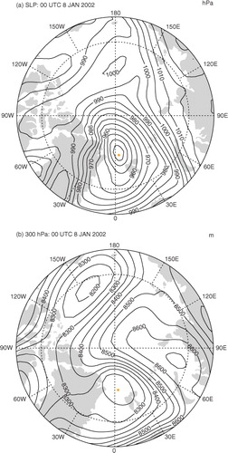
Table 1. Statistics the SLP cyclone with the lowest pressure (R1) in the 12 calendar months, for the period 1979–2009, with the time (UTC), date and year in which they occur, as determined by method M10

SLP cyclone				Z300 cyclone
Time	Date	Month	Year	Min. press. (hPa)	Anom.	Long. (°E)	Lat. (°N)	Min. Z300 (m)	Anom.	Long. (°E)	Lat. (°N)	Separation (km)
00	08	Jan	2002	938.0	−68.9	5.1	81.4	8222.5	−199.7	4.5	81.3	19.7
12	07	Feb	1995	946.8	−59.8	39.8	70.3	8101.0	−464.2	33.8	70.9	232.6
12	07	Mar	1997	947.3	−58.0	352.2	71.0	8301.2	−304.7	348.2	71.4	148.3
18	12	Apr	1990	953.5	−62.0	16.7	81.1	8254.1	−350.2	17.2	81.2	14.8
06	21	May	1998	964.9	−48.8	75.2	75.6	8508.5	−259.1	75.6	75.7	18.5
12	05	Jun	1994	970.2	−41.2	172.2	83.1	8494.6	−422.5	134.0	84.7	476.5
06	04	Jul	2002	974.5	−36.9	218.2	81.5	8587.2	−460.0	219.0	80.9	68.4
06	07	Aug	1995	966.7	−44.5	87.0	82.2	8650.0	−370.0	59.1	79.9	536.1
06	23	Sep	1982	957.7	−50.0	31.5	73.7	8635.5	−302.9	31.2	74.1	46.8
12	27	Oct	2003	950.9	−56.6	3.6	74.6	8408.0	−349.1	0.6	75.4	117.5
06	17	Nov	1996	942.5	−72.7	115.9	80.4	8123.8	−372.4	111.9	80.7	80.1
00	23	Dec	1990	940.6	−65.7	349.4	74.4	8241.5	−336.4	351.6	73.4	127.8

The fifth to eighth columns show the lowest central pressure, the deviation from the relevant monthly climatology at the location of the storm, and the longitude and latitude of the storm. The next four columns present analogous statistics for a vortex which was identified at the same time at the 300 hPa level in the vicinity of the surface storm. The last column displays the horizontal separation between the centres of the SLP and 300 hPa systems.

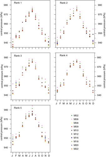
In comparing the identification of the most extreme storms in the 10 schemes, it is of value to examine the range of minimum pressures diagnosed by the different algorithms across the year. This information is presented in Fig. 2 for the five deepest cyclones separately. The central pressure determined for these calendar–month extremes show a relatively smooth variation through the year with, as might be expected, the lowest values in January (with an average across the schemes of 937.9 hPa for the R1 storm of 8 January 2002), to a July R1 maximum of 974.4 hPa). As would be expected the seasonality of the R2, R3, R4 and R5 storm plots are very similar. As indicated above, the different approaches taken in the identification methods (including the nature of the spatial interpolation of the pressure field) lead to a significant range of central pressure estimates for each of these 12 cyclones. The greatest range of central pressures for R1, 9.2 hPa, occurs in December. The range is smallest in summer but is still sizeable, with typical values of 5 hPa. Given the greater intensity of the storms in winter one would have expected this larger spread of estimated central pressures in that season. Another feature that is apparent in the Figure is that for R1 the relative ordering of the schemes with respect to their pressures tends to remain similar throughout the year. For example, methods M06 and M18 are inclined to have the highest central pressures, while the lowest are typically found in M12, M16 and M22. Even though all schemes start with the ERA-Interim as the basic data, many of the algorithms interpolate that data to their own native grids before the analysis is undertaken. Hence, the identified central pressure will depend to some extent on the resolution and disposition of the native grid (Kouroutzoglou et al., 2011). This, in part, explains the ranges observed. Another aspect of this is that, as pointed out above, the M06 scheme uses only 12-hourly data and hence may miss the full magnitude of the extremes. Note that when this analysis is applied to the four lower ranked cyclones, similar biases between the schemes are found to those identified for R1 (see the remaining panels in Fig. 2).

Fig. 2 Central pressure (hPa) of the R1, R2, R3, R4 and R5 cyclones in the 12 calendar months determined by each of the cyclone identification algorithms.

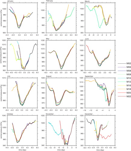
We now compare the evolution of the central pressure across the time at which the minimum occurs in the R1 cyclones, as diagnosed in the 10 schemes (regardless of whether the cyclone is inside or outside the Arctic). Figure 3 shows that these time series are similar in most months, even when the nature of the time series is quite complex. There are some differences as to when algorithms first identify the track, and when the cyclone decays, but these are seen only in one or two algorithms. In a few of the months while these outlier algorithms identify the same storm at the time of minimum pressure, they make different tracking choices in the lead up to the minimum (associated with the complexity of the SLP distribution at the time). Hence, the earlier parts of these few tracks pertain to cyclones which are not the same as those identified in all the other schemes. This contributes significantly to the apparent spread of SLP.

Fig. 3 Time series of the central pressure of cyclone identified in the methods in the time leading up to and after the minimum. The abscissa presents the time in days, and the zero represents the time of the minimum surface pressure.

For the extraordinary cyclones identified here, considerable interest centres on whether this group of intense Arctic storms has lifetimes differing from those of unexceptional storms, bearing in mind that Simmonds and Rudeva (2012) noted the most intense August storm lasted some 13 d. Note that their storm occurred in 2012, and hence is outside the analysis period we use here. In addition, we examine how those lifetimes differ between the various methods, particularly in light of the fact that, as we have just discussed, algorithms make different decisions as to the timing of genesis and decay. Table 2 displays the lifetime from genesis to lysis (in days) for our 12 R1 storms. An unbiased estimate of the lifetime (in days) presented here has been determined by (N/4), where N is number of consecutive (6-hourly) points along the storm track. One can see that estimates of the longevity of storms differ according to the method used. The longest-lived storm, when averaged over all the methods, was that in August, with a mean lifetime of 9 d. All the late spring and summer storms have mean lifetimes in excess of 6 d. By contrast the cyclones outside this period last a somewhat shorter time (about 4–6 d), with the shortest mean lifetime of a little over 4 d occurring in December. Overall, these lifetimes of extreme cyclones are longer than the winter population mean of about 2 d documented by Shkolnik and Efimov (2013). The relatively fleeting nature of the non-summer extreme storms means that these were, necessarily, rapidly intensifying systems. As we would have expected from the earlier discussion, there is a substantial difference in the mean R1 lifetimes diagnosed in the tracking algorithms; these vary from 4.63 d in M08 to 8.41 d in M12. The longest-lived storm was 19.5 d, identified in September 1982 by M18. The Tables for the other four rankings (not shown) exhibit similar overall structure to that in Table 2.

Table 2. Lifetime (in days) of the 12 R1 storms identified by the 10 identification methods

Mon	M02	M06	M08	M09	M10	M12	M16	M18	M20	M22	Max.		Ave.
Jan	8.25	4.75	3.50	3.75	5.00	4.25	4.00	5.50	4.00	3.50	8.25	M02	4.65
Feb	5.75	4.25	2.25	10.00	7.00	11.00	6.50	6.25	3.00	4.75	11.00	M12	6.07
Mar	8.50	6.25	2.00	2.50	2.25	9.00	8.75	6.00	2.50	2.25	9.00	M12	5.00
Apr	9.50	3.25	4.75	5.00	6.25	9.25	8.75	2.00	3.25	5.25	9.50	M02	5.72
May	6.25	6.25	6.25	9.75	7.25	10.25	7.25	7.00	9.75	9.75	10.25	M12	7.97
Jun	7.25	6.75	4.00	8.25	6.50	8.25	5.25	8.00	9.50	8.25	9.50	M20	7.20
Jul	8.25	7.25	6.50	6.50	3.25	6.75	6.75	9.25	6.50	6.50	9.25	M18	6.75
Aug	10.50	5.75	6.25	10.25	10.25	10.75	10.50	10.50	5.00	10.00	10.75	M12	8.98
Sep	12.00	9.75	8.75	3.25	10.25	7.75	3.00	19.50	4.75	5.00	19.50	M18	8.40
Oct	9.50	6.75	7.75	8.00	3.25	6.25	9.25	5.00	8.00	8.00	9.50	M02	7.18
Nov	7.00	1.75	1.50	7.50	17.25	9.00	−1	2.00	10.75	8.75	17.25	M10	7.28
Dec	7.75	2.75	2.00	6.00	3.50	−1	2.00	3.00	6.25	5.00	7.75	M02	4.25
Max	12.00	9.75	8.75	10.25	17.25	11.00	10.50	19.50	10.75	10.00
Sep	Sep	Sep	Aug	Nov	Feb	Aug	Sep	Nov	Aug
Ave	8.38	5.46	4.63	6.73	6.83	8.41	6.55	7.00	6.10	6.42

An unbiased estimate of lifetime is obtained by calculating N/4, where N is the number of consecutive (6-hourly) analyses in which the 12 storms are identified in the methods. Bold numbers denote the maximum for a given scheme, and Italics denotes the maximum for a given month, while Bold and italics indicate the maximum for a given month and scheme. Red font means that the cyclone was ranked the second or the third in that scheme, while ‘ −1’ indicates that the cyclone was not found in that scheme.

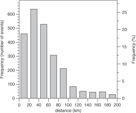
We commented above that, because of a number of factors, the various identification methods will locate the storm centres at somewhat different locations. We show in Fig. 4 composited data pertaining to the separation of the locations where the individual schemes identify their minimum pressure. The histogram displays the frequency bins for the separation for all possible pairs of identification methods for the top five ranked cyclones for all 12 months. Almost half (45%) of all the comparisons result in separations of less than 40 km, while 87% of comparisons are less than 100 km. The Figure demonstrates that there is robust agreement amongst the algorithms as to location of the centre.

Fig. 4 Histogram of the frequency bins for the separation between the locations of minimum central pressure in the various cyclone methods. The distribution is drawn from all available comparisons for the top five ranked cyclones and for all 12 such months.

Our sample is, however, small and hence it may be difficult to discern any meaningful trends as to when our storms occur in the three-decade record. We remark, however, that only three fall in the 2000s and the last of these is 2003. Similar results are found for the R2, R3, R4 and R5 cyclones. To pursue this we test the null hypothesis that the (population) mean of all the year numbers of the months in the reanalysis set (January 1979–March 2009) does not differ from the mean of the 12 years of the R1 storms (these two means are 1993.63 and 1995.33, respectively). Using the t-test we calculate t=0.30, and hence accept the null hypothesis of no statistically significant difference between the means. (The mean year of the entire set of 60 storms is 1993.53, and the difference is not significant in this case also.) In this limited context (the extreme end of the cyclone spectrum) this is consistent, as far as it goes, with studies which have revealed equivocal, or no net robust, change in Arctic basin cyclonicity (e.g. Simmonds et al., 2008; Vavrus et al., 2012; Vavrus, 2013).

Table A1. Code numbers for the tracking methods used in this study, and the main references for method descriptions

Code	Main references for method description
M02	Murray and Simmonds (1991), Pinto et al. (2005)
M06	1997), Hewson and Titley (2010)
M08	2006)
M09	Serreze (1995), Wang et al. (2006)
M10	Murray and Simmonds (1991), Simmonds et al. (2003)
M12	2002), Rudeva and Gulev (2007)
M16	2002)
M18	1994, 1997)
M20	2006)
M22	2005), Akperov et al. (2007)

4. Association of tropopause polar vortices with extreme Arctic surface cyclones

We earlier referred to the extensive evidence that vortices at the tropopause level can have significant influence on the development of surface systems, in addition to the forcings associated with low-level baroclinicity and turbulent fluxes of energy at the surface. We raise the question as to what extent are TPVs associated with the extreme Arctic storms studied here. Simmonds and Rudeva (2012) have already shown that the intense storm of August 2012 was intimately involved with a TPV, but that only represents one case. We are, however, in a position to ascertain to what extent our 60 extreme cyclones were associated with an upper-level system at a similar location. Because the IMILAST database was restricted to SLP cyclones, our investigation of this was restricted by the fact that we could perform a comparable 300 hPa geopotential height (Z300) cyclone analysis only with the M10 method (the Arctic tropopause is close to the 300 hPa level). Keable et al. (2002), Lim and Simmonds (2007), Kouroutzoglou et al. (2012) and Flocas et al. (2013) have shown that M10 can be applied successfully to upper-troposphere cyclone identification, whereas such comprehensive upper-level assessments have not been undertaken with the other algorithms. This analysis was undertaken for the same period and reanalysis as the surface cyclone identification, and the tests for vertical associations was undertaken with the technique described by Lim and Simmonds (2007). For each of our SLP cyclones a search was made for significant Z300 cyclones within a distance of 1000 km of the surface system.

For the R1 storms, this matching exploration found associated upper-level systems for all 12 cases. Fig. 1b shows the Z300 map and the TPV for the January case. Table 1 presents specific information on these Z300 vortices in the same form as presented for the SLP storms. The central height values convey that these are major cyclones, and represent significant anomalies the Z300 climatological values for that month and location (−199.7 m in January to −464.2 m in February). The Table reveals that there is strong vertical organisation and co-location between the SLP and tropopause cyclones, and the horizontal distance between them is as little as 14.8 km in the April 1990 case. In fact, storms at the two levels are separated by less than 100 km in six of the cases, less than 150 km in nine of the 12 cases, and the maximum separation is 536 km. As pointed out earlier, at the surface the greatest pressure anomalies occur in the winter semester and the smallest during summer. By contrast, Table 1 reveals no clear seasonality in the height anomalies of the TPVs.

For the entire set of 60 storms similarly robust associations are identified. Figure 5 shows that a significant proportion of the upper-level systems (denoted by crosses) are located almost directly above the surface feature (filled circles) at their times of maximum intensity, and all but six are to be found with 555 km (while all but three are within 1000 km).

Fig. 5 Locations of the five most intense surface cyclones for each of the calendar months (filled circles). The five colours denote the five rankings (see legend). The crosses denote the location of a significant Z300 system within 1000 km of the surface cyclone.

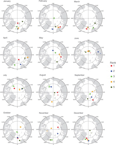
Table A2. Times and dates of the first, second, third, fourth and fifth highest ranked cyclone (R1, R2, R3, R4 and R5) for the 12 calendar months of the year

R1	R2	R3	R4	R5
Month	HH DD YYYY	HH DD YYYY	HH DD YYYY	HH DD YYYY	HH DD YYYY
Jan	00 08 2002	12 08 1993	12 11 1984	18 21 1994	00 13 2009
Feb	06 07 1995	18 06 1981	18 22 1996	18 28 1990	12 01 1993
Mar	12 07 1997	00 13 1995	00 01 1990	12 03 1979	12 22 2003
Apr	18 12 1990	18 04 2007	00 01 1995	00 04 1990	12 26 1997
May	00 21 1998	06 22 1992	18 02 1990	06 30 1994	06 04 2001
Jun	12 05 1994	12 19 1997	18 22 2008	12 08 1992	18 16 1986
Jul	06 04 2002	06 02 1986	18 29 2003	18 26 1992	18 05 1993
Aug	18 06 1995	18 28 1980	18 06 1991	00 22 1991	18 07 1994
Sep	06 23 1982	00 25 2003	06 28 1989	06 29 1986	12 02 1999
Oct	12 27 2003	18 12 1986	00 10 1988	18 28 1997	12 12 1996
Nov	06 17 1996	06 08 2004	12 10 2001	00 29 1993	06 28 1984
Dec	00 23 1990	00 20 1993	00 28 1980	12 23 2004	00 22 1979

‘HH’ denotes UTC time, ‘DD’ day of the month, and ‘YYYY’ year.

5. Impact of the extreme cyclones on the sea ice distribution

The focus of this study has been on properties of the most intense Arctic storms throughout the year, and to compare these properties as diagnosed by 10 state-of-the-art cyclone tracking schemes. However, it is worth commenting on the extent to which this small sample of atypical surface systems can have an impact on the sea ice distribution.

Over recent decades the climate of the Arctic region has exhibited significant changes, this being marked in the dramatic reduction of the sea ice extent. Walsh (2013) has commented that ‘sea ice has emerged as the canary in the coal mine of climate change’. Many climatological aspects of the Arctic climate system are interrelated in complex ways, and this certainly applies to sea ice and cyclones. Whether sea ice is present or not can potentially impact on the magnitude of the sensible heat flux and moisture flux across the atmosphere–ocean boundary, and hence on the energy available to cyclones. By contrast, on average, cyclones have a potential impact on sea ice by, for example, rearranging the ice pack and opening up leads.

We have explored the extent to which our exceptional sample of storms can be shown to impact on ice over their short life. To this effect we have examined the time rate of change of sea ice concentration (SIC) at the time of these storms, using the National Snow and Ice Data Center (NSIDC) data set (Meier et al., 2013). Overall, there were no robust signals in these tendencies (not shown). At first sight this may appear somewhat surprising. However, the response to a particular storm will depend on the SIC itself, and in regions of high concentration the ice is not free to be impacted by a short-lived cyclone. In their case study Dierer et al. (2005) commented on the intricacies of the ice response to cyclones and how these depend on SIC and sea ice properties themselves. Another aspect of this issue, which has been revealed in the recent literature, is that the nature of the sea ice response to storms depends very much on the preconditioning that the region has undergone (e.g. Howell et al., 2013; Parkinson and Comiso, 2013; Zhang et al., 2013). It is important to note that these extreme storms do not always have an impact on the surface fluxes. For example, Simmonds and Rudeva (2012) showed that the passage of the intense Arctic storm of August 2012 had little impact on the turbulent fluxes. The above discussion is not to say that an intense storm cannot strongly influence the SIC distribution, as indeed we have shown in past studies (e.g. Simmonds and Drinkwater, 2007), and often case studies are chosen because they exhibit a sea ice response. Kriegsmann and Brümmer (2014) performed a comprehensive statistical analysis of the effect of 3496 cyclones and revealed complex and subtle relationships between storms and SIC, which varied with location, season, ice thickness etc. It is not surprising that our small sample of very unusual cyclones do not reveal a signal which can be discerned above the noise.

6. Concluding remarks

This study has reported on the analysis of a subset of Arctic cyclones undertaken with 10 state-of-the-art cyclone identification schemes. Our intercomparison is conducted on the five most intense Arctic cyclone for each of the 12 calendar months over the 30-yr period from 1 January 1979 to 31 March 2009 in the ERA-Interim reanalysis. The task of identifying and tracking very intense Arctic cyclones is a difficult one for a number of reasons, one of which is that many of these systems develop and decay rapidly and hence schemes that are favourable to early detection may present a somewhat different picture of their climatological properties. More generally, as numerous authors have commented, there are many differences in the structure and behaviour of Arctic systems compared with more commonly-studied midlatitude cyclones (e.g. Tanaka et al., 2012). Most of the cyclone identification schemes in common use have been developed in a midlatitude context.

It is found that the central pressure, averaged over the 10 tracking schemes, of these most intense storms have a strong seasonal cycle, ranging from 937.9 hPa (in January) to 974.4 hPa (July). The magnitude of anomalies of the central pressures from the climatological mean for the relevant month at the location of storm centre also exhibits a strong seasonality, ranging from −72.7 to −36.9 hPa for the months of November and July, respectively. There is a sizable difference between the central pressures diagnosed by the 10 algorithms showing a range of estimates of about 5 hPa in summer and up to 9.2 hPa in December.

The evolution of the central pressure about the time at which the minimum occurs is encouragingly similar in the 10 schemes. A similar remark is true for the period in which the cyclones begin their decay. There were some outliers to this, however, and these deviations tended to be either very early or very late in the track. Some schemes showed a propensity to identify cyclones very early, and we have identified a range of diagnosed lifetimes for the same cyclone. However, very long lifetimes may be a result of merging two or more cyclones into one long track. When averaged over all schemes the lifetime of the R1 systems ranged from 4–8 d over most of the year, and tended to be longest in late spring and summer. The longest average length was 9 d for the August case. The broad agreement between the various algorithms extended to the estimated location of the central pressure at the time of greatest intensity. To quantify this for a given calendar month we took the 10 estimates of the location (from our set of identification algorithms) and then calculated the separations of all the pairs of these locations. This process was repeated for all the calendar months, and the separations composited. It was found that almost 90% of these pairings were separated by less than 100 km at the time of their maximum development in the Arctic basin.

Our study has found that 54 of our 60 extreme surface cyclones were, at the time of maximum intensity, closely co-located (within 555 km) with an intense tropopause vortex. This result is consistent with many theoretical and observational investigations. For practical reasons (the IMILAST archive only holds sea level cyclones) we were able to undertake this aspect of the analysis with only one algorithm, but the message is very clear that these intense surface systems were intimately associated with strong upper-level structures.

The investigation has highlighted some significant differences between the outputs of the algorithms. Taking the perspective that the 10 schemes used here are ‘equally good’, these diagnosed differences point to the value of using multiple identification schemes in the study of cyclone behaviour. This is particularly important as the community moves towards identifying Arctic cyclones and their properties in high resolution regional analyses (see, e.g. Tilinina et al., 2014).

7. Acknowledgements

We thank Swiss Re for sponsoring the IMILAST project (both with respect to its coordination office and workshops) and ECWMF for providing the ERA-Interim reanalysis. Parts of this research were made possible by a grant from the Australian Research Council.

8. Appendix

In Table A1 we present the main references for the design and description of the 10 cyclone identification and tracking methods used in this study. Table A2 lists the times and dates of the 60 extreme cyclones (rankings R1, R2, R3, R4 and R5) for the 12 calendar months of the year for the period 1 January 1979 to 31 March 2009.

References

- Akperov M. G. , Bardin M. Y. , Volodin E. M. , Golitsyn G. S. , Mokhov I. I . Probability distributions for cyclones and anticyclones from the NCEP/NCAR reanalysis data and the INM RAS climate model. Izvest. Atmos. Ocean. Phys. 2007; 43: 705–712.
- Bardin M. Y. , Polonsky A. B . North Atlantic Oscillation and synoptic variability in the European–Atlantic region in winter. Izvest. Atmos. Ocean. Phys. 2005; 41: 127–136.
- Cavalieri D. J. , Parkinson C. L . Arctic sea ice variability and trends, 1979–2010. Cryosphere. 2012; 6: 881–889.
- Cavallo S. M. , Hakim G. J . Composite structure of tropopause polar cyclones. Mon. Weather Rev. 2010; 138: 3840–3857.
- Cavallo S. M. , Hakim G. J . Radiative impact on tropopause polar vortices over the Arctic. Mon. Weather Rev. 2012; 140: 1683–1702.
- Cavallo S. M. , Hakim G. J . Physical mechanisms of tropopause polar vortex intensity change. J. Atmos. Sci. 2013; 70: 3359–3373.
- Comiso J. C . Large decadal decline of the Arctic multiyear ice cover. J. Clim. 2012; 25: 1176–1193.
- Dee D. P. , Uppala S. M. , Simmons A. J. , Berrisford P. , Poli P. , co-authors . The ERA-interim reanalysis: configuration and performance of the data assimilation system. Q. J. Roy. Meteorol. Soc. 2011; 137: 553–597.
- Dierer S. , Schlünzen K. H. , Birnbaum G. , Brümmer B. , Müller G . Atmosphere–sea ice interactions during a cyclone passage investigated by using model simulations and measurements. Mon. Weather Rev. 2005; 133: 3678–3692.
- Duarte C. M. , Agusti S. , Wassmann P. , Arrieta J. M. , Alcaraz M. , co-authors . Tipping elements in the Arctic marine ecosystem. Ambio. 2012; 41: 44–55.
- Flocas H. A. , Kountouris P. , Kouroutzoglou J. , Hatzaki M. , Keay K. , co-authors . Vertical characteristics of cyclonic tracks over the eastern Mediterranean during the cold period of the year. Theor. Appl. Climatol. 2013; 112: 375–388.
- Hewson T. D . Objective identification of frontal wave cyclones. Meteorol. Appl. 1997; 4: 311–315.
- Hewson T. D. , Titley H. A . Objective identification, typing and tracking of the complete life-cycles of cyclonic features at high spatial resolution. Meteorol. Appl. 2010; 17: 355–381.
- Hodges K. I . Feature tracking on the unit sphere. Mon. Weather Rev. 1995; 123: 3458–3465.
- Howell S. E. L. , Wohlleben T. , Komarov A. , Pizzolato L. , Derksen C . Recent extreme light sea ice years in the Canadian Arctic Archipelago: 2011 and 2012 eclipse 1998 and 2007. Cryosphere. 2013; 7: 1753–1768.
- Inoue J. , Hori M. E. , Enomoto T. , Kikuchi T . Intercomparison of surface heat transfer near the Arctic Marginal Ice Zone for multiple reanalyses: a case study of September 2009. SOLA. 2011; 7: 57–60.
- Jackson J. M. , Allen S. E. , McLaughlin F. A. , Woodgate R. A. , Carmack E. C . Changes to the near-surface waters in the Canada Basin, Arctic Ocean from 1993–2009: a basin in transition. J. Geophys. Res. 2011; 116: 10008.
- Jakobson E. , Vihma T . Atmospheric moisture budget in the Arctic based on the ERA-40 reanalysis. Int. J. Climatol. 2010; 30: 2175–2194.
- Keable M. , Simmonds I. , Keay K . Distribution and temporal variability of 500 hPa cyclone characteristics in the Southern Hemisphere. Int. J. Climatol. 2002; 22: 131–150.
- Kew S. F. , Sprenger M. , Davies H. C . Potential vorticity anomalies of the lowermost stratosphere: a 10-yr winter climatology. Mon. Weather Rev. 2010; 138: 1234–1249.
- Kouroutzoglou J. , Flocas H. A. , Keay K. , Simmonds I. , Hatzaki M . On the vertical structure of Mediterranean explosive cyclones. Theor. Appl. Climatol. 2012; 110: 155–176.
- Kouroutzoglou J. , Flocas H. A. , Simmonds I. , Keay K. , Hatzaki M . Assessing characteristics of Mediterranean explosive cyclones for different data resolution. Theor. Appl. Climatol. 2011; 105: 263–275.
- Kriegsmann A. , Brümmer B . Cyclone impact on sea ice in the central Arctic Ocean: a statistical study. Cryosphere. 2014; 8: 303–317.
- Lim E.-P. , Simmonds I . Southern Hemisphere winter extratropical cyclone characteristics and vertical organization observed with the ERA-40 reanalysis data in 1979–2001. J. Clim. 2007; 20: 2675–2690.
- Lionello P. , Dalan F. , Elvini E . Cyclones in the Mediterranean region: the present and the doubled CO2 climate scenarios. Clim. Res. 2002; 22: 147–159.
- Livina V. N. , Lenton T. M . A recent tipping point in the Arctic sea-ice cover: abrupt and persistent increase in the seasonal cycle since 2007. Cryosphere. 2013; 7: 275–286.
- Meier W. , Fetterer F. , Savoie M. , Mallory S. , Duerr R. , co-authors . NOAA/NSIDC Climate Data Record of Passive Microwave Sea Ice Concentration, Version 2. 2013; National Snow and Ice Data Center. Online at: https://nsidc.org/data/docs/noaa/g02202_ice_conc_cdr/ .
- Mesquita M.d. S. , Atkinson D. E. , Simmonds I. , Keay K. , Gottschalck J . New perspectives on the synoptic development of the severe October 1992 Nome storm. Geophys. Res. Lett. 2009; 36: 13808.
- Murray R. J. , Simmonds I . A numerical scheme for tracking cyclone centres from digital data. Part I: development and operation of the scheme. Aust. Meteorol. Mag. 1991; 39: 155–166.
- Neu U. , Akperov M. G. , Bellenbaum N. , Benestad R. , Blender R. , co-authors . IMILAST: a community effort to intercompare extratropical cyclone detection and tracking algorithms. Bull. Am. Meteorol. Soc. 2013; 94: 529–547.
- Parkinson C. L. , Comiso J. C . On the 2012 record low Arctic sea ice cover: combined impact of preconditioning and an August storm. Geophys. Res. Lett. 2013; 40: 1356–1361.
- Pezza A. B. , Simmonds I. , Renwick J. A . Southern Hemisphere cyclones and anticyclones: recent trends and links with decadal variability in the Pacific Ocean. Int. J. Climatol. 2007; 27: 1403–1419.
- Pinto J. G. , Spangehl T. , Ulbrich U. , Speth P . Sensitivities of a cyclone detection and tracking algorithm: individual tracks and climatology. Meteorol. Z. 2005; 14: 823–838.
- Raible C. C. , Della-Marta P. M. , Schwierz C. , Wernli H. , Blender R . Northern Hemisphere extratropical cyclones: a comparison of detection and tracking methods and different reanalyses. Mon. Weather Rev. 2008; 136: 880–897.
- Rudeva I. , Gulev S. K . Climatology of cyclone size characteristics and their changes during the cyclone life cycle. Mon. Weather Rev. 2007; 135: 2568–2587.
- Screen J. A. , Simmonds I . The central role of diminishing sea ice in recent Arctic temperature amplification. Nature. 2010; 464: 1334–1337.
- Screen J. A. , Simmonds I. , Keay K . Dramatic interannual changes of perennial Arctic sea ice linked to abnormal summer storm activity. J. Geophys. Res. 2011; 116: 15105.
- Serreze M. C . Climatological aspects of cyclone development and decay in the Arctic. Atmos. Ocean. 1995; 33: 1–23.
- Shkolnik I. M. , Efimov S. V . Cyclonic activity in high latitudes as simulated by a regional atmospheric climate model: added value and uncertainties. Environ. Res. Lett. 2013; 8: 045007.
- Simmonds I . Comparing and contrasting the behaviour of Arctic and Antarctic sea ice over the 35-year period 1979–2013. Ann. Glaciol. 2015; 56: 18–28.
- Simmonds I. , Burke C. , Keay K . Arctic climate change as manifest in cyclone behavior. J. Clim. 2008; 21: 5777–5796.
- Simmonds I. , Drinkwater M. R . Côté J . A ferocious and extreme Arctic storm in a time of decreasing sea ice. Research Activities in Atmospheric and Oceanic Modelling, Report No. 37, WMO/TD-No. 1397. 2007; Geneva: World Meteorological Organization. 2.27–2.28.
- Simmonds I. , Keay K . Extraordinary September Arctic sea ice reductions and their relationships with storm behavior over 1979–2008. Geophys. Res. Lett. 2009; 36: 19715.
- Simmonds I. , Keay K. , Lim E.-P . Synoptic activity in the seas around Antarctica. Mon. Weather Rev. 2003; 131: 272–288.
- Simmonds I. , Rudeva I . The great Arctic cyclone of August 2012. Geophys. Res. Lett. 2012; 39: 23709.
- Sinclair M. R . An objective cyclone climatology for the Southern Hemisphere. Mon. Weather Rev. 1994; 122: 2239–2256.
- Sinclair M. R . Objective identification of cyclones and their circulation intensity, and climatology. Weather Forecast. 1997; 12: 595–612.
- Skific N. , Francis J. A . Drivers of projected change in Arctic moist static energy transport. J. Geophys. Res. 2013; 118: 2748–2761.
- Tanaka H. L. , Yamagami A. , Takahashi S . The structure and behavior of the Arctic cyclone in summer analyzed by the JRA-25/JCDAS data. Polar Sci. 2012; 6: 55–69.
- Thorncroft C. D. , Hoskins B. J. , McIntyre M. E . Two paradigms of baroclinic-wave life-cycle behaviour. Q. J. Roy. Meteorol. Soc. 1993; 119: 17–55.
- Tilinina N. , Gulev S. K. , Bromwich D. H . New view of Arctic cyclone activity from the Arctic system reanalysis. Geophys. Res. Lett. 2014; 41: 1766–1772.
- Trigo I. F . Climatology and interannual variability of storm-tracks in the Euro-Atlantic sector: a comparison between ERA-40 and NCEP/NCAR reanalyses. Clim. Dyn. 2006; 26: 127–143.
- Vavrus S. J . Extreme Arctic cyclones in CMIP5 historical simulations. Geophys. Res. Lett. 2013; 40: 6208–6212.
- Vavrus S. J. , Holland M. M. , Jahn A. , Bailey D. A. , Blazey B. A . Twenty-first-century Arctic climate change in CCSM4. J. Clim. 2012; 25: 2696–2710.
- Walsh J. E . Melting ice: what is happening to Arctic sea ice, and what does it mean for us?. Oceanography. 2013; 26: 171–181.
- Wang X. L. , Swail V. R. , Zwiers F. W . Climatology and changes of extratropical cyclone activity: comparison of ERA-40 with NCEP-NCAR reanalysis for 1958–2001. J. Clim. 2006; 19: 3145–3166.
- Wernli H. , Schwierz C . Surface cyclones in the ERA-40 dataset (1958–2001). Part I: novel identification method and global climatology. J. Atmos. Sci. 2006; 63: 2486–2507.
- Woods C. , Caballero R. , Svensson G . Large-scale circulation associated with moisture intrusions into the Arctic during winter. Geophys. Res. Lett. 2013; 40: 4717–4721.
- Zhang J. , Lindsay R. , Schweiger A. , Steele M . The impact of an intense summer cyclone on 2012 Arctic sea ice retreat. Geophys. Res. Lett. 2013; 40: 720–726.
- Zolina O. , Gulev S. K . Improving the accuracy of mapping cyclone numbers and frequencies. Mon. Weather Rev. 2002; 130: 748–759.