Random projections in reducing the dimensionality of climate simulation data

Abstract

Random projection (RP) is a dimensionality reduction method that has been earlier applied to high-dimensional data sets, for instance, in image processing. This study presents experimental results of RP applied to simulated global surface temperature data. Principal component analysis (PCA) is utilised to analyse how RP preserves structures when the original data set is compressed down to 10% or 1% of its original volume. Our experiments show that, although information is naturally lost in RP, the main spatial patterns (the principal component loadings) and temporal signatures (spectra of the principal component scores) can nevertheless be recovered from the randomly projected low-dimensional subspaces. Our results imply that RP could be used as a pre-processing step before analysing the structure of high-dimensional climate data sets having many state variables, time steps and spatial locations.

• random projection
• principal component analysis
• dimensionality reduction
• climate simulation data
• El Niño – Southern Oscillation

1. Introduction

Climate simulation data are often high-dimensional, with thousands of time steps and grid points representing the state variables. High dimensionality is of course desirable, but it also presents a problem by making post-processing computations expensive and time-consuming. Data dimensionality reduction methods are therefore attractive, since they may enable the application of elaborate data analysis methods to otherwise prohibitively high-dimensional data sets.

Principal component analysis (PCA), also known as empirical orthogonal function (EOF) analysis (e.g. Rinne and Karhila, 1979; Von Storch and Zwiers, 1999), has been widely used in climate science in order to extract the dominant components of climate data time series. With large data sets, this method is computationally expensive, and rather soon becomes non-applicable unless the dimension of the original data set is significantly reduced. The use of time averaging, such as monthly or annual means instead of the original daily data, is an example of dimension reduction that sometimes enables PCAs use. This, however, significantly distorts the original information content of the data set: all temporal variability shorter than the averaging period is lost, and periods longer than the averaging period are affected. Thus, time averaging is not necessarily an optimal dimension reduction method.

This paper studies random projection (RP) as a dimensionality reduction method. It has been successfully applied in image processing (Bingham and Mannila, 2001; Goel et al., 2005; Qi and Hughes, 2012) and for text data (Bingham and Mannila, 2001). RPs fall into the theory of compressive sampling (CS), which has emerged as a novel paradigm in data sampling after the publications of Candès et al. (2006) and Donoho (2006). CS relies on the idea that most data have an inherent structure which can be viewed as sparsity. This means that, for example, a continuous signal in time may carry much less information than suggested by the difference between its upper and lower frequencies (Candès and Wakin, 2008; Bryan and Leise, 2013).

The aim of this paper is to introduce RP as a dimensionality reduction method in climate science. We will present the basic theory behind RP, and apply the method to climate data and show how the projected data preserve the essential structure of the original data. This is demonstrated by applying PCA to the original and randomly projected low-dimensional data sets to show that the leading principal components of the original data set can be recovered from the lower dimensional subspace. Section 2 presents the RP and PCA methods. In Section 3, we show some experimental results of applying RP and PCA to the original and dimensionality-reduced data sets. In addition, Section 4 demonstrates the application of the RP method to a very high-dimensional data set that represents multiple atmospheric model layers simultaneously.

2. Methods

2.1. Random projections

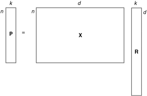
Random projection means that the n×d original data matrix (X) of n d-dimensional observations is projected by a d×k random matrix (R) (where k<d) to produce a lower dimensional subspace P of n×k:1

In RP we are projecting our data set onto k random directions defined by the column vectors of R. From these projections we can construct a lower dimensional representation of the original data set. The computational complexity of RP is of the order of O(knd). Due to the simplicity of RP, involving only matrix multiplication, it can be applied to a wide range of data sets, even those with a very high number of dimensions. Figure 1 illustrates how the dimensionality of the data matrix is reduced by RP.

Fig. 1 Dimensionality reduction by random projection. Original data X is projected onto a random matrix R to have a lower dimensional subspace P.

The idea of RPs stems from the Johnson–Lindenstrauss lemma (Johnson and Lindenstrauss, 1984):

Suppose we have an arbitrary matrix . Given any , there is a mapping f: , for any , such that, for any two rows x _i , , we have 2 In the lemma it is stated that the data points in d-dimensional space can be embedded into a k-dimensional subspace in such a way that the pairwise Euclidean distances between the data points are approximately preserved with a factor of . (See, e.g., Dasgupta and Gupta (2003) for proof of this result.)

Work has been done on finding suitable constructions of such mappings f (e.g. Frankl and Maehara, 1988; Achlioptas, 2003). In our experiments, we have employed a commonly used mapping (R) which consists of the vectors of normally distributed N(0,1) random numbers and the row vectors of the random matrix are scaled to have unit length. There are also other random distributions that satisfy the lemma [eq. (2)]. For example, Achlioptas (2003) has shown that a matrix of elements (r _ij ) distributed as3

satisfies the requirements of a suitable mapping.

It should also be noted that in eq. (1) we are assuming an orthogonal projection, although the column vectors of R are not perfectly orthogonal. Here we can rely on a theorem of Hecht-Nielsen (1994) stating that as the dimension of the space increases, the number of almost orthogonal vectors increases. According to Bingham and Mannila (2001), the mean squared error between RR ^T and an identity matrix is about 1/k per matrix element. We can therefore assume that the vectors of R are sufficiently orthogonal for the projection to work. It is also possible to orthogonalise the vectors of R, but it is computationally expensive.

We should also address the question of number of subdimensions (k) needed to get a representation of the original data set that is accurate enough. Some estimates can be found in the literature. Originally, Johnson and Lindenstrauss (1984) showed that the lower bound for k is of the order of . There has also been some work on revealing an explicit formula for k. For example, Frankl and Maehara (1988) came up with the result that is sufficient to satisfy the Johnson–Lindenstrauss theorem, while Dasgupta and Gupta (2003) showed that is enough. It is notable that the estimates of k depend only on the number of data points (observations) n, and are independent of d.

2.2. Principal component analysis

PCA is a widely used method to extract the dominant spatio-temporal signals from multidimensional data sets and to reduce the dimensionality of the data. In climate science, the principal component loadings are also known as empirical orthogonal functions (e.g. Rinne and Karhila, 1979; Von Storch and Zwiers, 1999).

PCA is based on the idea of finding a basis to represent the original data set (Shlens, 2009). The aim is to find latent variables that explain most of the variance in the original data set via uncorrelated linear combinations of the original variables (Hannachi et al., 2007). This also enables dimensionality reduction, as most of the variance in the data set can be explained by only a small subset of principal components.

One of the techniques for finding the principal components of the data matrix is singular value decomposition (SVD). SVD is based on a theorem stating that any matrix X _n×d can be broken down into orthogonal matrices U _n×n and V _d×d and a diagonal matrix D _n×d :4

where the columns of V are orthonormal eigenvectors of C=X ^T X (C is the covariance matrix of X), the columns of U are orthonormal eigenvectors of Z=XX ^T and D is a diagonal matrix containing the square roots of the eigenvalues of C or Z in descending order. Since the column vectors of V are the eigenvectors of C, SVD is a direct way of computing the PCA of the original data matrix X. The column vectors of V are also known as the PC loading vectors, and the PC score matrix S can be calculated as follows:5 As already mentioned, the PC loadings are also known as the EOFs (e.g. Rinne and Järvenoja, 1986) in which case the data set is often represented as a function of space (l) and time (t)6 where fm is a mean field, v _i is the spatial function of the i ^th component (i.e. the PC loading) and the s _i are time-dependent coefficients associated with v _i . The number of EOFs is denoted by w. If the EOF series is truncated, that is, the data set is projected onto a subset of PC loadings, a residual term is included.

In PCA, it is generally recommended to use a mean-centred data matrix (Varmuza and Filzmoser, 2009). If the data matrix is not centred, then typically the PCs resulting from the PCA are not uncorrelated with each other and the eigenvalues do not indicate variance but rather the non-central second moments of the PCs (Cadima and Jolliffe, 2009). In uncentred PCA, it is often the case that the first eigenvector (PC loading) is close to the direction of the vector of column means of the data matrix.

The computational complexity of PCA (implemented by SVD) is of the order of , but there are also computationally less-expensive methods for finding only a certain number of eigenvalues and vectors (see e.g. Bingham and Mannila (2001) and references therein). The aim of this study is to compare the results of normal PCA (implemented by SVD) applied to the original and dimensionality-reduced (RP + PCA) data sets. The computational complexity of the latter can be expressed as O(knd)+. Now the original dimensions are reduced from d to k, which means computational savings in the PCA.

PCA has its own limitations in providing interpretability of the physical patterns. Because of spatial orthogonality and temporal uncorrelation, the PCs do not necessarily correspond to any physical phenomena or patterns (Demšar et al., 2013). The constraint in PCA for the successive components to explain the maximum remaining variance may lead to a mixing of physical phenomena in the extracted PCs (Aires et al., 2000). There are several methods to overcome these limitations, e.g. rotating the PC loadings. It has also been argued that the decorrelation assumption of PCA is not enough, and that the statistical independence of the extracted components is needed to analyse the dynamical complexity of physical phenomena (Aires et al., 2000). However, in this study we are more concerned with demonstrating the RP method with the aid of PCA, and therefore we only utilise the normal PCA without any rotations. The focus is more on the method than on the physical interpretation of the data.

3. Comparison of the original and the projected data

3.1. Data

A monthly surface temperature data set from a millennial full-forcing Earth system model simulation (Jungclaus, 2008) was used in this experiment. The original monthly archived simulation data set has 14 472 time steps, but we selected for our use only 4608 time steps (the dimension n) from the end of the data set. The simulation data set has a resolution of 96 points in longitude and 48 points in latitude, resulting in 4608 locations or grid points (the dimension d). The dimensions n and d were chosen to be of equal size so that they could be reduced with RP equivalently. The 4608×4608 data matrix is quite large, but it is still manageable when performing PCA on it for comparison with the projected lower dimensional subspaces. Surface temperature was chosen because it has some well-known global patterns (e.g. El Niño – Southern Oscillation, ENSO) that can be identified with PCA.

3.2. Applying RP and PCA to the climate simulation data set

RP was applied in two different ways: the original data matrix was arranged so that (1) the time steps n were in the rows and the spatial locations d (gridpoints) were in the columns and (2) the locations were in the rows and the time steps in the columns. In this way, it was possible to project the data matrix in order to correspondingly reduce either the spatial (case 1) or the temporal (case 2) dimension, since with RP we can only reduce one dimension at a time. The original data matrix was mean-centred before projection on the lower dimensional subspace.

When the PCA of the original data matrix is calculated, the PC loading vectors give us the spatial maps corresponding to the PC scores. The PC score vectors are the projections of the original data matrix onto the PC loadings, and the scores can be presented as time series. After the dimensionality of the data matrix is reduced by RP, we have then reduced either the temporal or the spatial dimension. Therefore it is not possible to get the corresponding PC scores and loadings when the other dimension has been reduced. Using SVD to find the PCs of the dimensionality-reduced data set P _n×k , where the spatial dimension d has been reduced, gives us7 The loading vectors in V cannot be plotted on the original grid because we are now in instead of [see the Johnson–Lindenstrauss lemma; eq. (2)]. If the temporal dimension is reduced, we have P _k×d and the score vectors cannot be presented as time series comparable to the original PC scores. However, in the Appendix we present a novel method whereby the loadings (or scores) can be approximated by calculating the matrices U (or V) and D in the lower dimensional subspace and then multiplying these with the original data set. This method is applied in Section 4.

The number of subdimensions k needed for RP was discussed in Section 2.1. If we follow the bound given in Dasgupta and Gupta (2003), with an arbitrary value ɛ=0.2 and n=4608, the Johnson–Lindenstrauss theorem gives a limit of k=4(ɛ ²/2–ɛ ³/3)⁻¹ log n≈1947 (42% of the original dimensions) to make the projections with an accuracy of 1±ɛ. However, our experiments will show that, with our data set, a much smaller k still gives good results, recovering most of the information of the original data set. In this work, we are not looking for an exact lower bound for RPs applied to our data set but instead we are interested in demonstrating the method itself, keeping practical applications in mind. We therefore chose the dimensions for the RPs to be 10% and 1% of the original dimensions (4608). These percentages are equivalent to k≈460 (hereafter denoted as RP10%) and k≈46 (RP1%).

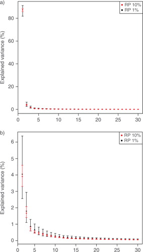
In order to investigate the stability of the results obtained by RPs, the original data matrix was projected onto 100 different realisations of RP matrices of the same k (where k is 46 or 460). For the uncertainty estimation, the original data matrix was arranged as in case 1. The PCA of each projection was calculated, making it possible to approximate the mean and the 95% confidence limits for the amount of variance explained by the PCs (Fig. 2). These confidence limits describe the uncertainties that arise from different projection matrices. From Fig. 2 we can see that the results can be somewhat different depending on what kind of RP matrix has been used. Some differences are to be expected, since the elements in the RP matrix are always different, although normally distributed N(0,1). Furthermore, as the projection dimension k increases, the 95% confidence intervals (of the same k) become narrower.

Fig. 2 Uncertainties of random projections. Mean and 95% confidence limits of the variance explained by the PCs (a) 1–30 and (b) 2–30 calculated from 100 realisations of projections of RP10% and RP1%. The explained variance of the first eigenvalue is excluded from subfigure (b) to show more details. In RP, the spatial dimension of the original data matrix is reduced.

3.3. Results of PCA

3.3.1. Explained variance of PCs.

The eigenvalues of the data covariance matrix are in descending order and indicate the significance, that is, the amount of variance, of the principal components. An essential part of EOF studies (e.g. Hannachi, 2007) is to analyse the eigenvalues in the detection of the dominant signals or patterns in climate data.

Figure 3 shows the percentage of explained variance of the PCs with their 95% confidence limits approximated from the original and projected data sets (RP10% and RP1%). The confidence limits are based on bootstrapping where the original and projected data sets are re-sampled 100 times with replacement and the PCA of each bootstrap sample is calculated. The sampling is done with respect to the temporal dimension and the obtained samples are arranged in chronological order. In the case of the projected data sets, the variances of the PCs are obtained using one realisation of each projection (RP10% and RP1% and cases 1 and 2 of both). We have also re-sampled these realisations of projected data matrices to analyse the uncertainties related to these specific projections. Notice the difference to the previous section, where we estimated the uncertainties of RP due to regenerated random matrices. In Fig. 3, we can see that in case 2, in which the temporal dimension n is reduced, the 95% confidence intervals become wider, as can be expected. Otherwise the confidence intervals are quite narrow because of large n.

Fig. 3 Explained variance of the 30 first PCs with their 95% confidence limits. (a–b) Original and RP10%, (c–d) Original and RP1%. The explained variance of the first eigenvalue is excluded from subfigures (b) and (d) to show more details. In RP, the spatial (1) and temporal (2) dimensions are reduced. The confidence limits are obtained by re-sampling the original and projected data sets 100 times, and the PCA of each sample is calculated.

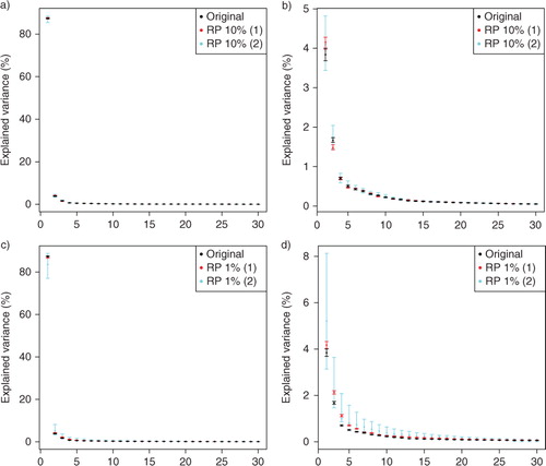
Figure 3 shows that the eigenvalues (illustrated as the percentage of the explained variance) decrease monotonically, and are quite similar in the cases of the original and projected data sets even when the dimension has been reduced to only 1% of the original dimensions. The eigenvalues of PCs 1–4 seem to be separated from the rest and also from each other, except in the case of RP1% with reduced temporal dimension n, where the 95% confidence limits of PCs 2 and 3, 3 and 4 as well as 4 and 5 overlap. The confidence limits of PCs 4 and 5 of RP10% with reduced n also overlap. PCs 1–4 explain almost 94% of the variance of the original and projected data sets. PC1 explains the majority (approximately 87%), PC2 4%, PC3 2% and PC4 approximately 1% of the variance. The rest of the eigenvalues decrease quite smoothly, which causes difficulties in distinguishing those small eigenvalues due to signal and those due to noise.

We saw that the eigenvalue spectra of the original and randomly projected data sets look quite similar. However, this only tells us that the amplitudes of the dominant signals are similar in both the original and the projected data sets. We also need to compare the PC loadings (i.e. the eigenvectors of the covariance matrix) and the PC scores to find out whether the spatio-temporal signatures have the same features.

3.3.2. PC loadings.

The PC loadings, or the spatial patterns of the PCs of the original and dimensionality-reduced data sets, are shown in Figs. 4 and 5. Visual inspection shows that the original data and RP10% have very similar spatial patterns of PCs 1–12, with some differences however in PCs 8 and 9. RP1% PCs have mostly similar spatial patterns with the original PCs up to component 5, subsequent loadings of RP1% having more deviations. It should be noted that a PC loading vector has an arbitrary sign. To facilitate comparison, some of the RP10% and RP1% loading vectors were multiplied by −1 if they correlated negatively with the original PC loading vectors.

Fig. 4 Spatial patterns of PC1–PC8 loadings. Comparison of the original, RP10% and RP1% data sets. In RP, the temporal dimension is reduced.

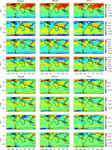
Fig. 5 Spatial patterns of PC9–PC12 loadings. Comparison of the original, RP10% and RP1% data sets. In RP, the temporal dimension is reduced.

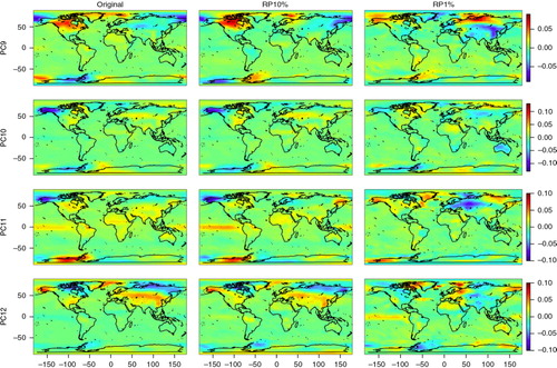
Spatial maps (especially PCs 4, 5, 6 and 11) show some features in surface temperature patterns that can be associated with the El Niño – Southern Oscillation (ENSO), e.g. distinct loadings in the Tropical Pacific and northwest/midwest North America (Trenberth and Caron, 2000). These same patterns can be found in the original, the RP10% and the RP1% maps and mostly in the same components.

The correlations of PC 1–20 loadings of the original and dimensionality-reduced (RP10% and RP1%) data sets are shown in Fig. 6. We can see that the RP10% loadings are strongly correlated with the original loadings until PC12 (correlation coefficient r>0.8 and r>0.9 up to PC7) and the RP1% loadings until PC5. PCs 1–5 already explain 94% of the variance of the data set and PCs 1–12 explain 96%. We can also see that some of the components of RP10%/RP1% have stronger correlations with adjacent ones of the original data set; for example, PC9 of RP10% has a stronger correlation with PC8 than with PC9 of the original data set. These adjacent components typically have similar variances.

Fig. 6 Correlation of the original and projected (RP10% and RP1%) PC loadings. In RP, the temporal dimension is reduced.

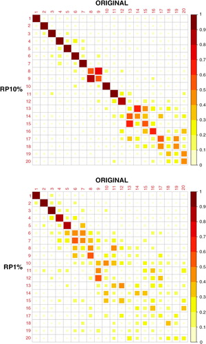
Results are in line with the findings of Qi and Hughes (2012), where it is theoretically verified that, although RP disperses the energy of a PC in different directions, the original PC remains as the direction with the most energy. Due to this, oscillations with similar variance can be assigned to different, adjacent components, leading to some ambiguity in the indices. Another, or supplemental explanation for the switching of adjacent PCs is provided in Jolliffe (1989). According to that paper, it is a well-known fact that PCs whose variances (or eigenvalues) are nearly equal are unstable, but their joint subspace is stable. It has been shown that small changes in the variances in this subspace can lead to large changes in corresponding PC loading vectors, and this may lead to the switching of adjacent PCs. Thus it is more important to detect the same oscillations and patterns in the original and projected data sets, not in having them assigned to exactly the same components.

3.3.3. PC scores.

The time series of PC scores were analysed with the Multitaper spectral analysis method (Thomson, 1982; Mann and Lees, 1996) to find the most powerful frequencies in these time series. The power spectra of the original and projected PC scores are shown in Fig. 7. Dominant features of the power spectra are the harmonic component frequencies which are integer multiples of the fundamental frequency. In the monthly surface temperature data set, the fundamental frequency is 1/12, which corresponds to a period of 1 yr and the harmonics clearly visible in the power spectra of PCs are 1/6, 1/4 and 1/3, corresponding to periods of 1/2, 1/3 and 1/4 yr that are related to intra-annual variations of surface temperature. The peaks at these frequencies are very similar in corresponding components of the original data, RP10% and RP1%. The peaks at the harmonics may also indicate that the orthogonality constraint of PCA is not suitable for this data set. The PCs are global and may have the same structure so that the first PC possesses the fundamental frequency while the following ones possess its harmonic frequencies (Aires et al., 2000).

Fig. 7 Spectra of PC1–PC12 scores. (a) The original data set, (b) RP10% and (c) RP1%. In RP, the spatial dimension is reduced.

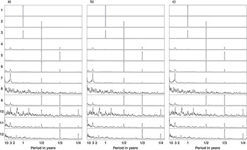
Apart from the seasonal/harmonic frequencies, there are distinct peaks in the PC score spectra around the period of 3 yr. This might be related to ENSO which has a cycle of 2–6 yr. These peaks are clearly distinguishable in PCs 6 (original), 7 (RP10% and RP1%) and 11 (original and RP1%) with some differences between the original and dimensionality-reduced data sets. We already identified some ENSO-related features in the spatial maps.

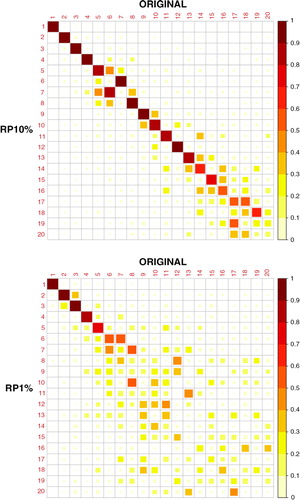
The correlations of the original and RP10%/RP1% PC scores (Fig. 8) are quite similar to the correlations in the loadings (Fig. 6). The RP10% correlations to the original scores are strong (r > 0.8) until about PC13, and PCs 6 and 7 are cross-correlated. The RP1% correlations with the original scores are also strong until PC5, although the correlation coefficient of PC5 is slightly less than 0.8.

Fig. 8 Correlation of the original and projected (RP10% and RP1%) PC scores. In RP, the spatial dimension is reduced.

4. Application of RP to a very high-dimensional data set

To demonstrate the application of the RP method to a very high-dimensional data set, we used a monthly temperature data set from a millennial full-forcing Earth system model simulation (Jungclaus, 2008) with a vertical resolution of 17 levels in the atmosphere between 1000 and 10 hPa. Inclusion of the vertical component increased the dimension d of the data matrix to 4608×17 = 78 336. We extracted 3600 time steps (n) from the end of the data set. The increase of d from 4608 to 78 336 makes in our case PCA non-applicable (in a laptop computer), and thus we call the dimension ‘very high’. Therefore the dimensionality of the data matrix was reduced by RP to make PCA applicable.

The original data matrix is X( n × d) with n=3600 and d=78 336, referring to time step and location, respectively. The dimensionality of the data matrix was reduced by projecting it onto a random matrix R(d×k), where k≈783 is the subspace dimension (1% of the original dimensions d) [eq. (8)]. We then calculated the SVD of the lower dimensional data P(n×k) to get the matrix U _RP (n×k) [eq. (9)]. The PC loadings V(d×k) were then approximated by multiplying the transpose of the original data matrix X(n×d) with U _RP (n×k) and the inverse of the diagonal matrix D _RP (k×k) which we got from the SVD of P [eq. (10)] (see Appendix).8 9 10 The diagonal elements of D _RP (k×k) are the square roots of the eigenvalues of the data covariance matrix indicating the significance of the PCs. Columns of U _RP (n×k) multiplied by D _RP (k×k) [see eq. (5)] are the PC scores: these are analysed with the Multitaper spectral analysis method (Thomson, 1982; Mann and Lees, 1996) as in Section 3. The columns of V(d×k) are the PC loading vectors, that is, the spatial patterns corresponding to the PC scores. The elements of a loading vector contain the spatial patterns of a certain PC at 17 standard pressure levels of the atmosphere. The first 1–4608 elements correspond to level 1 (1000 hPa), elements 4609–9216 correspond to level 2 (925 hPa), and so on until 10 hPa.

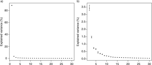
Figure 9 shows the percentage of the variance the PCs explain with their 95% confidence limits. The confidence limits were estimated by bootstrapping, as we did with the surface temperature data set in the previous section. PCs 1–3 are clearly separated from the rest and also from each other. PCs 4 and 5 (and maybe even PCs 6, 7 and 8 as their own subgroup) still seem to be distinguishable from the remaining eigenvalues which decrease quite smoothly. PC1 explains the majority of the variance in the data set (approximately 89%), PC2 explains 3.5%, PC3 approximately 1.5% and PCs 4 and 5 both explain approximately 0.7%. PCs 1–3 together account for 94% of the variance in the data set. The confidence intervals are narrow because of the relatively large sample size n.

Fig. 9 Explained variance (%) of PCs with their 95% confidence limits estimated by bootstrapping. PCs (a) 1–30 and (b) 2–30 of the three-dimensional atmospheric temperature data set (the spatial dimension is reduced by RP) are shown. The explained variance of the first eigenvalue is excluded from subfigure (b) to show more details.

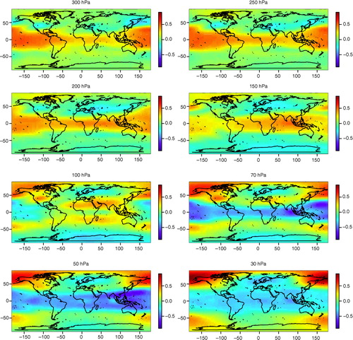
Figure 10 shows that the dominant frequencies of the atmospheric temperature variation are those related to annual and intra-annual oscillations, which were also detected in the surface temperature data set in the previous section. There are also peaks in the PC score spectra around the period of 3 yr which might be related to ENSO. The most distinct ENSO-related component is PC5 and its spatial patterns at the 1000–30 hPa levels are shown in Figs. 11 and 12. At the lower atmospheric levels, especially 1000–925 hPa, temperature patterns related to ENSO can be identified in the Tropical Pacific and northwest/midwest North America. At the 850–600 hPa levels the positive loadings near the equator decrease but again increase at levels from 500 to 250 hPa and at the same time spread both north- and southwards, especially in the Pacific. The North American pattern attenuates little by little, but is still identifiable up to 400 hPa. At the upper levels the loadings around the tropics and subtropics become negative, meaning that the oscillation in the upper atmosphere is in an opposite phase compared to lower levels, where the pattern is clearly positive in the same areas.

Fig. 10 Spectra of PC1–PC12 scores of the three-dimensional atmospheric temperature data set (the spatial dimension is reduced by RP).

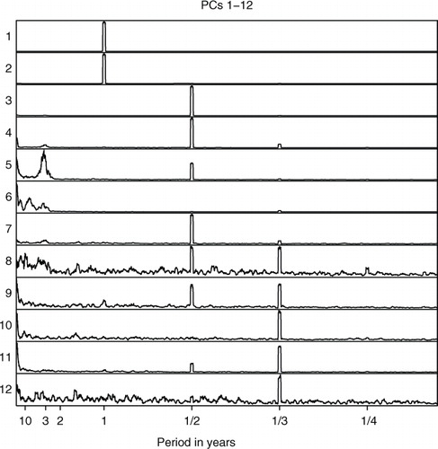
Fig. 11 The spatial patterns of the PC5 loadings of the atmospheric temperature data set (the spatial dimension is reduced by RP) between 1000 and 400 hPa. The spatial patterns are approximated using the method explained in the Appendix.

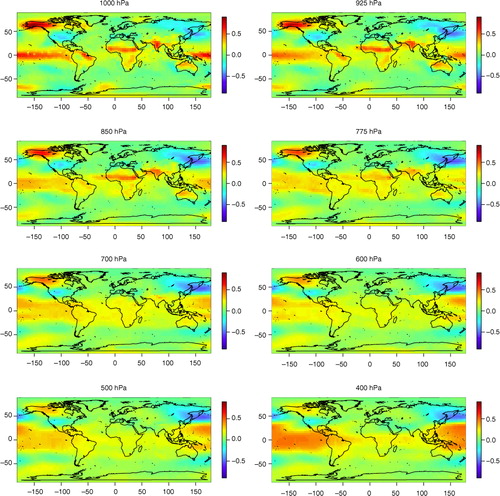
Fig. 12 The spatial patterns of the PC5 loadings of the atmospheric temperature data set (the spatial dimension is reduced by RP) between 300 and 30 hPa. The spatial patterns are approximated using the method explained in the Appendix.

Some caution is needed in the physical interpretation of these results. We already mentioned the limitations of PCA in Section 2.2. It should be noted that PC5 also has a distinct half-year peak, meaning that this component also carries an intra-annual signal. This is most likely to be related to the mixing problem of PCA. The ENSO representation of the model used in the simulations should also be considered (See, e.g., Jungclaus et al., 2006; Bellenger et al., 2014). Despite the limitations in the physical interpretation of the results, this experiment gives an example of how a large, multidimensional data set can be preprocessed with RP and then analysed efficiently to find, for example, the latent structures in the data set.

5. Summary and conclusions

The dimensionality of a simulated surface temperature data set was reduced by RP, and PCA was utilised to compare the structure of the original and projected data sets. Lower dimensional subspaces of 10% and 1% of the original data dimensions were investigated. The experiments showed that even at 1% of the original dimensions the main spatial and temporal patterns or principal components of the original surface temperature data set were approximately preserved. With a subspace of 10% of the original dimensions, we were able to recover the PCs explaining 96% of the variance in the original data set and with 1% we still could recover the PCs explaining 94% of the original variance.

The findings of this work are supported by the results presented in Qi and Hughes (2012). In their paper, it is theoretically and experimentally shown that a normal PCA performed on low-dimensional random subspaces recovers the principal components of the original data set very well, and as the number of data samples n increases the principal components of the random subspace converge to the true original components.

RP is computationally fast compared to other methods for dimensionality reduction (e.g. PCA) since it involves only matrix multiplication. It can therefore be applied to very high-dimensional data sets. Based on our experiments, it seems to open new possibilities in reducing the dimensionality of climate data. One of the topics of our forthcoming research is to investigate the applicability of RP before the use of some other computationally heavy analysis methods for multivariate climate data, for example, multichannel singular spectrum analysis (e.g. Ghil et al., 2002).

As mentioned, there are some estimates available for the lowest bound for the reduced dimensions k. These estimates depend on the number of observations (dimension n) in the original data set and the desired accuracy of the projection (controlled by error ɛ). These estimated bounds seem to be much higher than the ones we used with good results. This suggests that the bounds for dimensionality reduction with RP should be investigated in more detail in the case of climate data. We would then also need to know what is the information content of our data set, that is, the signals that rise above the noise in the original data set.

We also demonstrated the application of the RP method to a very high-dimensional data set of the atmospheric temperature in three dimensions. Our results imply that RP could be used as a pre-processing step before analysing the structure of large data sets. This might allow an investigation of the dynamics of truly high-dimensional climate data sets of several state variables, time steps and spatial locations.

Acknowledgements

This research has been funded by the Academy of Finland (project number 140771). We want to thank the two anonymous reviewers for their valuable comments and suggestions that helped in substantially improving the manuscript.

7. Appendix

A.1. Random projection and the singular value decomposition

In this Appendix we explain the method used in Section 4. Let's say we have an original data X _n×d . The singular value decomposition (SVD) of X is:A1

The covariance matrix of X is C=X ^T X and the columns of V are the eigenvectors of C. Also, the columns of U are the eigenvectors of Z=XX ^T . D is a diagonal matrix containing the square roots of the eigenvalues of C or Z in descending order.

Since the random projection (RP) of X is P=XR, where R _d×k is the projection matrix, (the row vectors of R are scaled to have unit length), we can write:A2 A3

In the previous we have assumed that RR ^T ≈ I, because the row vectors of R are nearly orthonormal. It is also possible to make the vectors of R strictly orthogonal, but this is computationally quite expensive.

Let's rewrite eq. (A1) as X _n×d =U _n×r D _r×r where r=rank(X). Now we can manipulate eq. (A1):A4 A5

Because Z≈Z _RP , we can approximateA6

In the previous we have defined U _RP as n×k and D _RP as a k×k matrix, where k is the rank of matrix P _n×k .

If we have a very high-dimensional data set X we can first reduce the dimensionality of X by RP and then approximate U (or V) and D in a lower dimensional subspace. We can then multiply the original data matrix with the approximated matrices U (or V) and D, finally getting the approximations of the PC scores or loadings depending on which dimension we have reduced in RP.

References

- Achlioptas D . Database-friendly random projections: Johnson–Lindenstrauss with binary coins. J. Comput. System Sci. 2003; 66: 671–687.
- Aires F. , Chedin A. , Nadal J. P . Independent component analysis of multivariate time series: application to tropical SST variability. J. Geophys. Res. 2000; 105: 17437–17455.
- Bellenger H. , Guilyardi E. , Leloup J. , Lengaigne M. , Vialard J . ENSO representation in climate models: from CMIP3 to CMIP5. Clim. Dynam. 2014; 42: 1999–2018.
- Bingham E. , Mannila H . Random projection in dimensionality reduction: applications to image and text data. Proceedings of the seventh ACM SIGKDD international conference on Knowledge discovery and data mining, KDD '01. 2001; New York: ACM. 245–250.
- Bryan K. , Leise T . Making do with less: an introduction to compressed sensing. SIAM Rev. 2013; 55: 547–566.
- Cadima J. , Jolliffe I . On relationships between uncentered and column-centered principal component analysis. Pak. J. Statist. 2009; 25: 473–503.
- Candès E. J. , Romberg J. , Tao T . Robust uncertainty principles: exact signal reconstruction from highly incomplete frequency information. IEEE Trans. Inform. Theory. 2006; 52: 489–509.
- Candès E. J. , Wakin M. B . An introduction to compressive sampling. IEEE Signal Process. Mag. 2008; 52: 21–30.
- Dasgupta S. , Gupta A . An elementary proof of a theorem of Johnson and Lindenstrauss. Random. Struct. Algorithm. 2003; 22: 60–65.
- Demšar U. , Harris P. , Brunsdon C. , Fotheringham A. S. , McLoone S . Principal component analysis on spatial data: an overview. Ann. Assoc. Am. Geogr. 2013; 103: 106–128.
- Donoho D . Compressed sensing. IEEE Trans. Inform. Theory. 2006; 52: 1289–1306.
- Frankl P. , Maehara H . The Johnson–Lindenstrauss lemma and the sphericity of some graphs. J. Combin. Theor. Series B. 1988; 44: 355–362.
- Ghil M. , Allen M. R. , Dettinger M. D. , Ide K. , Kondrashov D. , co-authors . Advanced spectral methods for climatic time series. Rev. Geophys. 2002; 40: 1–40.
- Goel N. , Bebis G. , Nefian A . Face recognition experiments with random projection. Defense and Security. International Society for Optics and Photonics. 2005; 426–437.
- Hannachi A . Pattern hunting in climate: a new method for finding trends in gridded climate data. Int. J. Climatol. 2007; 27: 1–15.
- Hannachi A. , Jolliffe I. T. , Stephenson D. B . Empirical orthogonal functions and related techniques in atmospheric science: a review. Int. J. Climatol. 2007; 27: 1119–1152.
- Hecht-Nielsen R . Context vectors: general purpose approximate meaning representations self-organized from raw data. Computational Intelligence: Imitating Life, IEEE Press. 1994; 43–56.
- Johnson W. , Lindenstrauss J . Extensions of Lipschitz mappings into a Hilbert space. Conference in modern analysis and probability (New Haven, Conn., 1982). 1984; Contemporary Mathematics: American Mathematical Society. 189–206.
- Jolliffe I. T . Rotation of Ill-defined principal components. J. Roy. Stat. Soc. Series C (Applied Statistics). 1989; 38: 139–147.
- Jungclaus J . MPI-M earth system modelling framework: millennium full forcing experiment (ensemble member 1). 2008; World Data Center for Climate. CERA-DB “mil0010”. Online at: http://cera-www.dkrz.de/WDCC/ui/Compact.jsp?acronym=mil0010.
- Jungclaus J. H. , Keenlyside N. , Botzet M. , Haak H. , Luo J.-J. , co-authors . Ocean circulation and tropical variability in the coupled model ECHAM5/MPI-OM. J. Clim. 2006; 19: 3952–3972.
- Mann M. E. , Lees J. M . Robust estimation of background noise and signal detection in climatic time series. Clim. Change. 1996; 33: 409–445.
- Qi H. , Hughes S. M . Invariance of principal components under low-dimensional random projection of the data. Proceedings of the 19th IEEE International Conference on Image Processing (ICIP). 2012; 937–940. IEEE.
- Rinne J. , Järvenoja S . A rapid method of computing empirical orthogonal functions from a large dataset. Mon. Weather. Rev. 1986; 114: 2571–2577.
- Rinne J. , Karhila V . Empirical orthogonal functions of 500 mb height in the northern hemisphere determined from a large data sample. Q. J. Roy. Meteorol. Soc. 1979; 105: 873–884.
- Shlens J . A tutorial on principal component analysis. 2009. Online at: http://www.snl.salk.edu/~shlens/pca.pdf.
- Thomson D. J . Spectrum estimation and harmonic analysis. Proc. IEEE. 1982; 70: 1055–1096.
- Trenberth K. , Caron J . The Southern Oscillation revisited: sea level pressures, surface temperatures, and precipitation. J. Clim. 2000; 13: 4358–4365.
- Varmuza K. , Filzmoser P . Introduction to Multivariate Statistical Analysis in Chemometrics. 2009; Boca Raton: CRC Press.
- Von Storch H. , Zwiers F. W . Statistical Analysis in Climate Research. 1999; Cambridge: Cambridge University Press.