Contrasting meridional structures of stratospheric and tropospheric planetary wave variability in the Northern Hemisphere

Abstract

The meridional structures of stratospheric and tropospheric planetary wave variability (PWV) over the Northern Hemisphere (NH) extratropics were investigated and compared using reanalysis data. By performing the spherical double Fourier series expansion of geopotential height data, the horizontal structures of PWV at each vertical level could be examined in the two-dimensional (2D) wavenumber (zonal and meridional wavenumbers) space. Comparing the amplitudes of wave components during the last three decades, the results suggested that the structures of PWV in the NH troposphere significantly differ from the stratospheric counterparts. The PWV in the troposphere shows multiple meridional wave-like structures, most pronounced for the meridional dipole; while in contrast, PWV in the stratosphere mainly shows large-scale zonal wave patterns, dominated by zonal waves 1 and 2, and have little wave-like fluctuation in the latitudinal direction. The dominant patterns of the NH PWV also show contrasting features of meridional structure between the stratosphere and the troposphere. As represented in the 2D wavenumber space, the leading two empirical orthogonal functions of PWV in the stratosphere largely exhibit the zonal wave 1 pattern, while those in the troposphere clearly show meridional wave-like structures and are dominated by the dipole. The refractive index was derived based on the zonal mean basic state to qualitatively interpret the observational findings. The results suggested that the basic state in the NH troposphere is much more favourable for latitudinally propagating stationary waves than the stratosphere. The difference in meridional structure between stratospheric and tropospheric planetary waves can be well captured in a linear baroclinic model with the observed zonal mean basic state. Furthermore, both theoretical and modelling analyses demonstrated that the fact that zonal wave patterns are preferred in the NH stratosphere may be partly attributable to the vertical curvature of the stratospheric zonal mean basic state.

• planetary waves
• stratosphere
• troposphere
• spherical double Fourier series
• two-dimensional wavenumber

1. Introduction

In the extratropical Northern Hemisphere (NH), atmospheric circulation variability in both the troposphere and stratosphere is closely linked with planetary wave variability (PWV), particularly during the cold season. Meanwhile, the PWV is important for the north–south transport of momentum, heat and mass (Chen and Huang, 2002; Randel et al., 2002), and is related to regional and hemispheric climates (Chen et al., 2005; Wang et al., 2009). Previous theoretical studies have suggested a significant influence of mid-latitude westerly flow on the propagation and evolution of planetary waves (Rossby, 1939; Yeh, 1949; Kuo, 1956; Charney and Drazin, 1961). The phase and group velocities of planetary waves are mainly determined by the magnitude of the zonal mean flow, and planetary wave propagation can possibly be controlled by meridional and vertical shears of the zonal wind. On the other hand, the impact of planetary waves on the zonal mean flow has also been theoretically demonstrated based on the wave–mean flow interaction theorem (Edmon et al., 1980; Andrews et al., 1987). The Eliassen–Palm flux and its divergence represent the propagation and absorption of planetary waves, which results in westerly deceleration or acceleration of the zonal mean flow.

Both theoretical and modelling studies have suggested that the tropospheric PWV over the extratropics may partly originate from the tropics. The Rossby wave ray theory provides a theoretical explanation for the influence of tropical sea surface temperature (SST) anomalies on tropospheric planetary waves (Hoskins and Karoly, 1981; Karoly, 1989). In particular, the meridional propagation of planetary waves in response to the prescribed tropical heating can be well explained by Rossby wave rays, which are established through the energy dispersion along a great circle on the sphere. The propagation speed and direction of Rossby wave rays depend primarily on the structure and strength of the zonal mean zonal wind. The impact of zonal mean flow change on the propagation of planetary waves has also been studied using both barotropic (Simmons et al., 1983) and baroclinic models (Nigam and Lindzen, 1989). In both cases, it can be found that the wave response to the prescribed heating is sensitive to the meridional structure of zonal mean basic flow. Moreover, the result obtained from the barotropic model linearised about the zonal mean flow in the upper troposphere is different compared with the corresponding baroclinic model result, suggesting an important role of the vertical structure of the zonal mean basic state (Ting, 1996). However, the relative influence of the meridional structure and the vertical structure of the zonal mean basic state on planetary waves in the stratosphere has not been fully revealed.

The enormous increase in observational data for the upper troposphere and stratosphere enables us to perform observational analyses on PWV. Because the El Niño–Southern Oscillation (ENSO) is one of the dominant modes of tropical SSTs, many investigations have focused on the relationship between the ENSO and planetary wave propagation over the extratropical NH (Chen et al., 2003; Garfinkel and Hartmann, 2007; Xie et al., 2012). Warming of eastern tropical Pacific SST is favourable for the strengthening of upward propagation into the stratosphere over NH high latitudes and the weakening of southward propagation in the NH troposphere. Besides the propagation, the horizontal structure of planetary waves is also important for understanding the variability of planetary waves and its relation to regional climates (Chen et al., 2005). Using one-dimensional (1D) Fourier series along longitude, planetary waves can be decomposed in terms of zonal wavenumbers. Some studies have revealed that planetary waves with zonal wavenumber 1 are dominant in the NH stratosphere, and planetary waves with zonal wavenumbers 1–3 show comparable amplitudes in the NH troposphere (Wang et al., 2009). However, the meridional structure of planetary waves cannot be depicted quantitatively using traditional 1D Fourier decomposition. It has been suggested that the meridional structure of planetary waves has an important impact on the meridional transport of water vapour and momentum over the extratropical NH (Boer et al., 2001; Kimoto et al., 2001). Moreover, as mentioned above, theoretical analyses have demonstrated that the meridional wave-like structure is critical for the dispersion of Rossby waves on a sphere (Hoskins and Karoly, 1981; Karoly, 1989), and the Rossby wave train dispersing along latitude has also been discussed extensively in terms of meridional teleconnection patterns (Wallace and Gutzler, 1981; Trenberth et al., 1998 and references therein). Observational studies in the literature have also suggested that a more coherent picture of the variability of planetary waves emerges only when one considers its full two-dimensional (2D) structure in the space domain, rather than solely its 1D structure along latitude circles (Wallace and Blackmon, 1983). Therefore, planetary waves should be regarded as 2D waves on a sphere for the examination of their meridional structures.

Few investigations of PWV characteristics in the 2D wavenumber space have been performed, mainly because the meridional structure is difficult to represent using a simple function. Recently, Sun and Li (2012) employed double Fourier series (DFS) on the sphere (Layton and Spotz, 2003; Cheong et al., 2004) to investigate the space–time features of Southern Hemisphere daily 500 hPa geopotential height and identified the dominant meridional structure associated with tropospheric intraseasonal variability. It has been suggested that the spherical DFS representation is simple and easy to relate to real atmospheric circulation patterns, compared with other 2D representation methods (e.g. spherical harmonics). Because spherical harmonic decomposition can only be performed on an entire sphere, the DFS method also has an advantage over spherical harmonics when applied to the extratropics. Thus, it is considered an effective method to investigate NH extratropical PWV characteristics in the 2D wavenumber space. Such investigations may help to advance our understanding of NH PWV, particularly the detailed meridional structures of PWV in both the troposphere and stratosphere, and provide new insight into the dynamics of important climate modes by using DFS representation.

The aim of this paper is to analyse NH tropospheric and stratospheric PWV and their differences in the 2D wavenumber space. We focus on meridional structures of PWV, which have not been highlighted in the previous literature. The remainder of the paper is organised as follows. The data and methods are introduced in Section 2. Section 3 describes the structures of NH tropospheric and stratospheric PWV in the 2D wavenumber space. Section 4 investigates the leading patterns of PWV in the NH stratosphere and troposphere and their differences in meridional structures. In Section 5, we interpret the results by performing both theoretical and modelling analyses. And finally, Section 6 draws conclusions from the present study and provides an outlook for future work.

2. Data, model and methodology

2.1. Data

In this study, we used monthly mean geopotential height and wind reanalysis data from the region poleward of 20°N, provided by the National Centers for Environmental Prediction–Department of Energy Global Reanalysis 2 (NCEP2, Kanamitsu et al., 2002) for the period from January 1979 to February 2010, and with a horizontal resolution of 2.5°×2.5°. The planetary wave fields were derived by removing the zonal means of geopotential height fields. Because we focus on the variability of planetary waves, monthly anomalies of eddy geopotential height were further derived by removing the mean seasonal cycle based on the 30-yr (1980–2009) monthly climatology. In addition, the analysis presented in this study focuses mainly on the interannual variability during the boreal winter season, because the low-frequency variability of NH atmospheric circulation tends to maximise during winter (Blackmon et al., 1979). Here, winter is defined as an average of December–January–February (DJF), and years for winter averages are equal to those of December. For example, the winter of 1979 refers to the average from December 1979 to February 1980. Geopotential height data from National Centers for Environmental Prediction–National Center for Atmospheric Research (NCEP–NCAR/NCEP1, Kalnay et al., 1996) and European Center for Medium Range Weather Forecasting (ECMWF) reanalysis dataset (ERA-Interim, Simmons et al., 2007) were also analysed to verify the reliability of the result based on the NCEP2 reanalysis product. Results from all the three reanalysis datasets are similar to each other, and thus we show only the results based on the NCEP2 datasets unless specified otherwise. We chose geopotential height fields at 10, 50 and 100 hPa as indicators of stratospheric circulation and height fields at 300, 500 and 700 hPa as indicators of tropospheric circulation.

We used the Niño 3.4 (area-average 5°N–5°S, 170°–120°W) index from the Kaplan SST dataset (Kaplan et al., 1998) to represent the ENSO variations. The Pacific/North American (PNA) index, defined in Wallace and Gutzler (1981) based on standardised 500-hPa geopotential height values in four centres of action, was obtained from http://jisao.washington.edu/data_sets/pna. The Quasi Biannual Oscillation (QBO) index was constructed by the equatorial zonal mean zonal wind at 50 hPa, as given by Holton and Tan (1980). The North Atlantic Oscillation (NAO) index used in this study is defined as the difference in the normalised sea-level pressure zonally-averaged over the NA sector from 80°W to 30°E between 35°N and 65°N, derived from the NCAR data set (Li and Wang, 2003; Wu et al., 2009; Li et al., 2013).

2.2. Statistical methods

In order to identify patterns of PWV in the NH stratosphere and troposphere, we performed empirical orthogonal function (EOF) analysis on the eddy geopotential height field (after removal of the zonal mean) at a given vertical level. The EOF analysis was applied to seasonal mean anomalies, and area weighting was accomplished by multiplying the eddy field by the square root of cosine of latitude (North et al., 1982a; Sun et al., 2013). The EOFs derived from the stratospheric (tropospheric) data are referred to as the S-EOFs (T-EOFs) for short, and the corresponding principle components are referred to as S-PCs (T-PCs). The capital letter ‘S’ indicates the stratosphere and the letter ‘T’ the troposphere.

The statistical significance of linear regression/correlation coefficients was evaluated using the Student's t-test, in which the effective degree of freedom, N _eff, is estimated as:1 where N is the sample size and ρ _XX (j) and ρ _YY (j) are the autocorrelations of two sampled time series, X and Y, at time lag j, respectively (Pyper and Peterman, 1998; Li et al., 2013). Equation (1) is usually applied to define the N _eff of order 2, as it is appropriate for significance tests involving second order moments of the original time series (e.g. variance, covariance, and correlation).

2.3. Linear baroclinic model and barotropic model

In order to examine the influence of the zonal mean basic state on the meridional structure of planetary waves, a linear baroclinic model (LBM) was employed in this study. The primitive equations in the LBM are those for vorticity, divergence, temperature and logarithm of surface pressure, and are linearised about a zonally uniform basic state. The LBM can be solved with an externally imposed forcing and obtains a steady response through adiabatic processes. Thus, it is an important diagnostic tool and widely used to simulate either anomalous or climatological stationary waves (Held et al., 2002). The LBM used here has a horizontal resolution of T21 and 20 sigma levels in the vertical direction. These vertical levels are distributed with an interval of 0.02 in the stratosphere (above 200 hPa) and an interval of 0.08 in the troposphere (below 200 hPa). The top and bottom levels are at σ=0 and σ=1, respectively. There is a sponge layer near the model top (σ=0.02) to minimise the reflection of waves. For simplicity, there is no topography specified for the experiments presented in this study. Three dissipation terms are included: a biharmonic horizontal diffusion with the damping time scale of 1 d for the smallest wave, a weak vertical diffusion, and the Newtonian damping and Rayleigh friction as represented by a linear drag. Details of the model formulation are given in Watanabe and Kimoto (2000).

The linear barotropic model is a stationary model with a horizontal resolution of T21 and consists of a simple barotropic vorticity equation given as:2 where J represents a Jacobian operator; and are basic state and perturbation streamfunctions, respectively; f is the Coriolis parameter, and is the anomalous vorticity source induced by the divergence. The biharmonic diffusion coefficient ν is chosen to be 2×10¹⁶ m² s⁻¹ in order to dampen the small-scale eddies at a time length/period comparable to 1 d, while the Rayleigh friction coefficient α is set to 10 d⁻¹ (Zuo et al., 2013).

2.4. Spatial spectral expansion

At a given level, the monthly eddy geopotential height anomaly on the sphere Z (λ,φ) is considered to be a function of longitude and latitude, where λ is longitude and is latitude. Using the DFS on a sphere, Z (λ,φ) can be represented by a sum of the Fourier series,3 where k and l are zonal and meridional wavenumbers, respectively, with their maximums denoted by K and L. C _k,l and S _k,l denote the coefficients of zonal cosine and sine waves, respectively. Φ is a linear function of φ, which is determined by north–south boundary conditions. A detailed description of the DFS decomposition of 2D fields can be found in Sun and Li (2012). In the current study, rigid boundary conditions were imposed at both the northern and southern boundaries, with the boundary values set to zero. Thus, , where =90°N and =20°N are latitude values at the northern and southern boundaries, respectively. K=20 and L=15 were adopted.

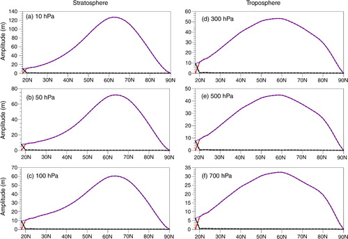
The eddy geopotential height anomaly can be well represented by the DFS in both the NH extratropical troposphere and stratosphere. Figure 1 shows the zonal means of the standard deviations of the monthly eddy geopotential height field, its DFS representation and zonal means of the root-mean-square deviation (RMSD) between the monthly observation and the DFS representation at different vertical levels. As seen in Fig. 1, the RMSD values are very small and almost equal to zero over the northern extratropics, demonstrating that the monthly eddy geopotential height fields are well represented. The geopotential height fluctuations at the southern boundary appear to be about one order of magnitude smaller than those at middle latitudes, indicating that the rigid boundary condition at the southern boundary is reasonable. The eddy geopotential height is identically zero at the North Pole, which is naturally consistent with the northern boundary condition of the DFS representation. The time series of the ratio of the total RMSD to the standard deviation over the NH domain (not shown here) also suggests that the truncation error is always small and that the variability of geopotential height is largely retained by the DFS representation. Therefore, the representation of the monthly eddy geopotential height anomaly via the spherical DFS can be considered to be adequate.

Fig. 1 (a) Zonal means of the standard deviations (m, blue thin line) of monthly 10 hPa eddy geopotential height anomalies (long-term mean seasonal cycle removed), the DFS representation of monthly height field (red dashed line), and zonal mean of the RMSD between the monthly observations and the DFS representation (black dashed line) from 1979 to 2009 over the NH extratropics. Panels (b)–(f) are the same as (a), but for 50, 100, 300, 500 and 700 hPa, respectively.

After the monthly or seasonal mean eddy geopotential height anomaly is decomposed into the DFS, the amplitudes of each wave component (k, l) can be calculated from the Fourier coefficients, C _k,l and S _k,l , as The difference in the amplitude among various wave patterns at a given vertical level actually reflects the relative contribution of each wave pattern to the 2D horizontal circulation. Larger amplitude for the set of (k, l) indicates that the corresponding wave pattern is the more dominant structure of the eddy geopotential height at the given vertical level. However, as seen in Fig. 1, and as suggested by previous studies (Hu and Tung, 2002; Wang et al., 2009), the amplitudes of planetary waves in the NH stratosphere always appear to be much larger than those in the troposphere, and thus, in this study, it is inadequate to compare the absolute amplitude values between stratospheric and tropospheric planetary waves and to show their respective dominant structures. Therefore, at a given vertical level, we normalise the amplitude of each wave component (k, l) by dividing the amplitude values by the maximum value among them, and refer them to as the normalised amplitudes. Among the wave patterns, modes for l=1 represent zonal wave patterns, and modes for l≠1 represent 2D waves with latitudinal wave-like structures.

3. Meridional structures of NH stratospheric and tropospheric PWV

Although some previous studies have mentioned the difference between the NH stratospheric and tropospheric atmospheric circulation patterns (e.g. Perlwitz and Graf, 1995), the extent to which the meridional structures of stratospheric PWV differ from those in the troposphere has not been quantified. Figure 2 shows the normalised amplitudes of winter (DJF) mean PWV in the 2D wavenumber (zonal and meridional wavenumbers) space. It can be seen that the normalised amplitudes show remarkable differences between stratosphere and troposphere, particularly for the meridional wavenumbers. In the NH stratosphere (Fig. 2a–c), the wave pattern of (k, l)=(1, 1) shows the strongest amplitude during winter, indicating that the zonal wave 1 is the most dominant structure of the eddy geopotential height variability. Perlwitz and Graf (1995) performed an EOF analysis on the full-field winter stratospheric circulation, and pointed out that the second and third EOFs closely resemble the zonal wave 1 (the first EOF describes the fluctuations of the zonally symmetric stratospheric vortex). Therefore, the important role of zonal wave 1 in the variability of stratospheric eddy geopotential height is further demonstrated in the 2D wavenumber space. Another feature, seen from Fig. 2a–c, is that as the altitude decreases in the stratosphere, the amplitude of zonal wave 2 becomes stronger, which suggests that zonal wave 2 makes an important contribution to the variability of lower stratospheric planetary waves. This is also consistent with previous findings that the stratospheric zonal wave 2 is one of the leading coupled modes of variability between lower stratospheric and tropospheric geopotential height fields (Perlwitz and Graf, 2001). Wave patterns with larger meridional wavenumbers (l>1) show very weak amplitudes compared with large-scale zonal wave patterns, suggesting that the PWV in the NH stratosphere has little wave-like fluctuation in the latitudinal direction. Based on these results, it is also implied that the dynamics of stratospheric PWV are mainly associated with large-scale zonal waves.

Fig. 2 (a) Climatological average over 31 (1979–2009) winters (DJF) of the wave amplitude as a function of k and l for the 10 hPa seasonal mean eddy geopotential height anomalies (long-term mean seasonal cycle removed) over the NH extratropics. The abscissa and ordinate represent zonal and meridional wavenumbers (k, l)=(1–5, 1–5), respectively. The amplitude values displayed in (a) have been divided by the maximum amplitude among all wave components (k, l). The maximum amplitude in (a) is 89 m for (k, l)=(1, 1). Panels (b)–(f) are the same as (a), but for 50, 100, 300, 500 and 700 hPa, respectively. The maximum amplitudes in (b)–(f) are 44 m for (k, l)=(1, 1), 24 m for (k, l)=(1, 1), 17 m for (k, l)=(1, 2), 14 m for (k, l)=(1, 2) and 11 m for (k, l)=(1, 2), respectively.

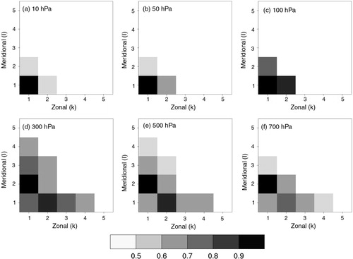
In sharp contrast, in the NH troposphere, planetary-scale quasi-stationary waves prefer latitudinal wave-like structures during winter, as clearly seen in Fig. 2d–f. The most intense amplitude is observed for the wave pattern of (k, l)=(1, 2), consistently from the lower to the upper troposphere, implying that the meridional structures of tropospheric PWV are dominated by north–south dipoles. Previous studies calculated the teleconnectivity of the NH tropospheric geopotential height fields in the longitude–latitude domain during the winter season and demonstrated that the low-frequency teleconnection patterns are always dipole shaped in the north–south direction, particularly over North Pacific and North Atlantic regions (Wallace and Gutzler, 1981; Blackmon et al., 1984; Athanasiadis and Ambaum, 2009). Thus, the meridional dipole structure is further identified as the most important feature of the tropospheric PWV in the 2D wavenumber space. The amplitudes of meridional modes (l>1) become small as the zonal wavenumber increases, suggesting modes with large total horizontal wavenumber () may have small amplitudes. The normalised amplitude associated with zonal wave 2 grows large as the altitude increases in the troposphere, showing that the zonal wave 2 is active in both the upper troposphere and lower stratosphere.

Figure 3 shows the time series of amplitude for wave patterns (k, l)=(1, 1–3) at the 50 and 500 hPa levels during NH winters. In the stratosphere, the zonal wave 1 pattern (k, l)=(1, 1) always shows the largest amplitude, further indicating that large-scale waves (k=1) in the stratosphere are dominated by zonal wave patterns rather than meridional wave-like patterns. It is also seen that the time series of amplitude for (k, l)=(1, 1) shows a positive trend in the last three decades, while the amplitudes for (k, l)=(1, 2–3) exhibit no statistically significant trends. As seen in Fig. 3b, the situation is different in the troposphere. Although the wave amplitudes show considerable interannual variations, the meridional dipole pattern (k, l)=(1, 2) has the strongest amplitude. Moreover, trend analyses of the time series in Fig. 3b show that there are no significant trends in the amplitudes for (k, l)=(1, 1–3) over the period 1979–2009. The wave amplitude time series from three different reanalysis datasets are highly correlated over the long-term period (Table 1), indicating that the temporal features of amplitudes of different wave components are broadly consistent in all three datasets.

Fig. 3 (a) Time series of the amplitudes for 50 hPa wave patterns with zonal wavenumber 1 (k=1) and different meridional wavenumbers (l=1–3 denoted by red, blue and black lines, respectively) during the winters from 1979 to 2009. (b) As in (a), but for the 500 hPa wave patterns.

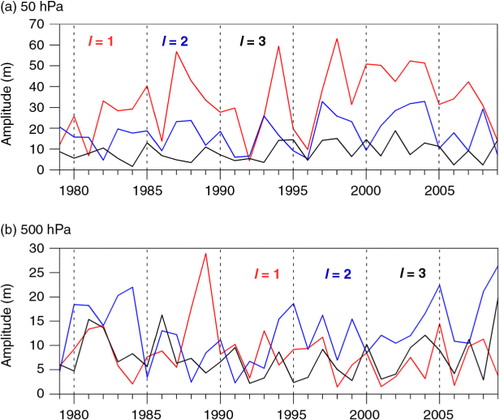
Table 1. Correlation coefficients for wave amplitude time series (k, l)=(1, 1–3) at 500 and 50 hPa between the NCEP2, NCEP1 and ERA-interim data sets during the winters of 1979–2009^a

l=1 at 500 (50) hPa	l=2 at 500 (50) hPa	l=3 at 500 (50) hPa
R(NCEP2, NCEP1)	0.95 (0.93)	0.96 (0.95)	0.94 (0.92)
R(NCEP2, ERA)	0.92 (0.89)	0.91 (0.88)	0.89 (0.87)
R(NCEP1, ERA)	0.90 (0.87)	0.89 (0.85)	0.86 (0.84)

^aAll correlation coefficients are statistically significant at the 95% confidence level.

The meridional structures of stratospheric and tropospheric PWV during other NH seasons were also examined. Figure 4a and b show the seasonal variations of wave pattern amplitudes for (k, l)=(1, 1–5) as a function of meridional wavenumber and calendar month at the vertical levels of 50 and 500 hPa, respectively. The amplitudes displayed in Fig. 4 were divided by the maximum amplitude value among all calendar months at each vertical level. A common feature in both NH stratosphere and troposphere is that the PWV is strong during boreal winter and weak during boreal summer (JJA). This feature is more evident in the NH stratosphere, where the amplitude of the PWV in JJA is about one order of magnitude smaller than that in DJF. The weak PWV during boreal summer has also been noted in previous studies (Perlwitz and Graf, 2001).

Fig. 4 (a) Seasonal evolution of climatologically averaged (1979–2009) wave amplitude (k, l)=(1, 1–5) as a function of l and calendar month for the 50 hPa eddy geopotential height anomalies (long-term mean seasonal cycle removed) over the NH extratropics. The abscissa and ordinate represent calendar month and meridional wavenumber, respectively. The amplitude values displayed in (a) have been divided by the maximum amplitude among all sets of l and calendar month. The maximum amplitude in (a) is 50 m for l=1 and February. (b) As in (a), but for 500 hPa. The maximum amplitude in (b) is 16 m for l=2 and February.

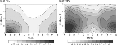
The differences in the meridional structure between stratospheric and tropospheric PWV for k=1 can still clearly be seen. In the NH stratosphere, the amplitude decreases rapidly as the meridional wavenumber increases during every calendar month, implying that the latitudinal wave-like fluctuations are always small, while zonal wave 1 plays an important role in the variability of stratospheric planetary waves. However, the amplitudes of tropospheric PWV do not change monotonously with the meridional wavenumber and in every calendar month the maximum amplitude is found for meridional wavenumbers l>1. Particularly, the amplitudes maximise at l=2 during winter and at l=3 during summer. This is to some extent consistent with the difference in the spatial scale between winter and summer teleconnection patterns. Teleconnection patterns in summer prefer to have a smaller meridional scale than their winter counterparts (Ogi, 2004; Folland et al., 2009). The results for other stratospheric levels (10 and 100 hPa) and tropospheric levels (300 and 700 hPa) were found to be similar to those for 50 and 500 hPa, respectively, and are thus not shown here.

In summary, PWV in the NH troposphere exhibits evident 2D Rossby wave patterns in the 2D wavenumber space, and thus shows multiple meridional structures, most pronounced for the meridional dipole during the cold season. However, in contrast, PWV in the NH stratosphere mainly shows zonal wave patterns and possesses little latitudinal wave-like fluctuation. Zonal wave 1 is the most prominent pattern of stratospheric PWV, while zonal wave 2 is active in the upper troposphere and lower stratosphere.

4. Comparing the leading patterns of PWV in the stratosphere and troposphere

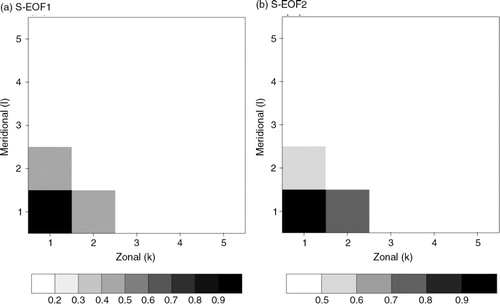
Section 3 described the PWV characteristics mainly from a climatological point of view. It has been known that the variability of atmospheric circulation appears to be dominated by some preferred recurrent patterns, such as teleconnection patterns (Wallace and Gutzler, 1981; Hannachi, 2010). Thus, it is interesting to examine the meridional structures of the leading patterns of PWV in the stratosphere and troposphere, respectively. Figure 5 shows the first two leading EOF modes of the 50 hPa winter eddy geopotential height anomalies in the NH stratosphere (hereafter referred to as S-EOF1 and S-EOF2). The first two modes account for 40 and 29% of the interannual variance, respectively, and according to the criterion of North et al. (1982b), the S-EOF1 and S-EOF2 are statistically distinct from each other and the rest of the eigenvectors in terms of the sampling error bars (not shown here). The S-EOF1 looks like a zonal wave 1 pattern with negative anomalies centred over Northeast America and positive anomalies over the Russian Far East. The S-EOF2 also features a zonal wave 1 pattern, but the phase appears to be shifted eastward by 90° compared with the S-EOF1 (based on the longitudes of the centres of action). The structures of the two EOF patterns can be identified more clearly in the 2D wavenumber space. As shown in Fig. 6, the zonal wave 1 pattern (k, l)=(1, 1) shows the strongest amplitude for both S-EOF1 and S-EOF2, further suggesting that the zonal wave 1 pattern prevails in the low-frequency modes of the NH stratospheric PWV.

Fig. 5 The (a) first and (b) second EOFs (S-EOF1 and S-EOF2) of the 50 hPa winter NH eddy geopotential height anomalies (poleward of 20°N) for the period 1979–2009, shown as regressions of the height fields onto the normalised EOF time series. (c) Normalised time series of the S-EOF1 (red) and QBO (blue) indices for the winters from 1979 to 2009. (d) As in (c), but for the S-EOF2 (red) and ENSO (blue) indices.

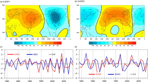
Fig. 6 Normalised wave amplitudes as a function of k and l for the 50 hPa eddy geopotential height anomaly associated with the (a) S-EOF1 and (b) S-EOF2 as shown in Fig. 5a and b. The abscissa and ordinate represent zonal and meridional wavenumbers, respectively.

Many studies have investigated the possible associations between tropical climate forcings and NH extratropical stratospheric variability. It has been suggested that both the ENSO and QBO have effects on the NH stratospheric polar vortex variability (Holton and Tan, 1980; van Loon and Labitzke, 1987; Garfinkel and Hartmann, 2007, 2008; Wei et al., 2007; Xie et al., 2012), which is closely related to the weakening/strengthening of the zonal mean flow. We further examined the possible relationship between the two tropical climate forcings and the leading EOFs of NH stratospheric PWV. Figure 5c shows the interannual time series of the QBO index and the time coefficients of the S-EOF1 for the winter season. The correlation between the S-EOF1 time series and the QBO index is 0.45, which is above the 95% confidence level, suggesting that the QBO variability contributes significantly to the S-EOF1 pattern. Several mechanisms have been suggested to be involved in the relationship between the QBO and stratospheric PWV over the NH extratropics. Holton and Tan (1980) showed that the subtropical critical wind line controlled by the QBO may affect the propagation of planetary waves from the troposphere into the stratosphere. The influence of the QBO's meridional circulation on planetary wave propagation has also been emphasised recently (Garfinkel et al., 2012). Figure 5d shows the winter time series of the ENSO and S-EOF2. The two indices are strongly correlated (r=0.5, above the 95% confidence level), indicating that the variability of S-EOF2 is partly attributable to the ENSO. Previous studies have suggested that the upward wave propagation from the troposphere to the stratosphere may provide a mechanism for the possible influence of the ENSO on stratospheric planetary waves (Garcia-Herrera et al., 2006; Manzini et al., 2006; Garfinkel and Hartmann, 2007; Ineson and Scaife, 2009). In addition, much smaller correlations are found between the S-EOF1 and ENSO as well as between the S-EOF2 and QBO (0.08 and −0.05, respectively). This implies that the effects of the QBO and ENSO on the leading two modes of NH stratospheric PWV may be separated. Moreover, according to the results in Fig. 6, it may be concluded that both the QBO and ENSO signals are implicated in the variability of the stratospheric zonal wave 1 pattern.

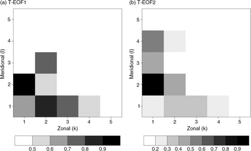
The structures of the leading EOF patterns of PWV in the troposphere are significantly different from the stratosphere. Figure 7 displays the first two EOF modes of the 500 hPa winter eddy geopotential height anomalies in the NH troposphere (hereafter referred to as T-EOF1 and T-EOF2). The results are similar if we choose other tropospheric levels (e.g. 300 and 700 hPa). The first two modes account for 25 and 16% of the total variance, respectively, and are statistically distinct from each other and the rest of the eigenvectors. The T-EOF1 shows centres of action mainly over the East Asia, North Pacific and North America, while the T-EOF2 shows maximum centres over the North Atlantic and northern Eurasia. The T-EOF1 and T-EOF2 somehow resemble the well-known PNA and NAO patterns, respectively. However, different from previous studies based on the full-field geopotential height (Wallace and Gutzler, 1981; Barnston and Livezey, 1987), T-EOF1 and T-EOF2 are derived based on wave fields with the zonal means removed prior to the analysis. It is evident that both T-EOF1 and T-EOF2 have meridional wave-like structures, which are in contrast with the stratospheric counterparts (S-EOF1 and S-EOF2). This contrasting feature becomes more apparent and quantitative in the 2D wavenumber space (Fig. 6 vs. Fig. 8). Much stronger normalised amplitudes for meridional waves with l>1, particularly for the meridional dipole (l=2), are clearly seen in both T-EOF1 and T-EOF2, indicating that the NH tropospheric low-frequency PWV is dominated by latitudinal dipole structures.

Fig. 7 (a) and (b) As in Fig. 4a and b, but for the leading two EOFs (T-EOF1 and T-EOF2) of the 500 hPa eddy geopotential height anomalies. (c) Normalised time series of the T-EOF1 (red) and ENSO (blue) indices for the winters from 1979 to 2009. (d) As in (c), but for the T-EOF2 (red) and NAO (blue) indices.

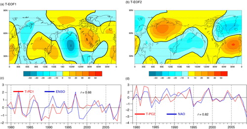
Fig. 8 Normalised wave amplitudes as a function of k and l for the 500 hPa eddy geopotential height anomalies associated with the (a) T-EOF1 and (b) T-EOF2 as shown in Fig. 7a and b. The abscissa and ordinate represent zonal and meridional wavenumbers, respectively.

We examined the possible connections between the ENSO and the leading EOFs of NH tropospheric PWV. As shown in Fig. 7c, T-EOF1 is strongly correlated with the ENSO variation (r=0.66, significant above the 95% confidence level). Moreover, the T-EOF1 pattern of Fig. 7a is reminiscent of the PNA, although it shows an additional centre of action in the East Asia. The PNA and ENSO are closely linked over the interannual timescale (r=0.63), and a significant positive correlation (r=0.65) is observed between the PNA and T-EOF1. It is well-known that the ENSO activity can excite PNA-like pattern in the extratropics according to the Rossby wave ray theory (Hoskins and Karoly, 1981; Simmons et al., 1983; Karoly, 1989), thus T-EOF1 can be understood as a Rossby wave response to eastern tropical Pacific SST variations.

The NAO is known as one of the dominant modes of atmospheric variability over the extratropical NH (Hurrell, 1995). Although the NAO occurs mainly over the North Atlantic region, it has been connected to the zonally symmetric NH annular mode (NAM, Thompson and Wallace, 2000; Wallace, 2000) and large-scale stationary waves (Ting et al., 1996; DeWeaver and Nigam, 2000). The T-EOF2 pattern of Fig. 7b looks like the NAO over North Atlantic, although it also has large amplitudes in the northern Eurasia. In addition, as shown in Fig. 7d, the time series of the winter NAO index and T-EOF2 are significantly correlated (r=0.82). Previous studies have suggested a downstream influence of the NAO on the Ural and Okhotsk blocking highs due to its modulation on the planetary waves, and that the Asian jet acts as a potential waveguide for the downstream propagation of Rossby waves (Watanabe, 2004; Wu et al., 2009, 2012). Thus, the large wave amplitudes over the northern Eurasia associated with T-EOF2 may be interpreted as the downstream response of planetary waves to the NAO. The high correlation between T-EOF2 and NAO also indicates that NAO-like variability may be obtained from wave fields alone.

Therefore, the results above suggest that the ENSO and NAO, two important modes of climate variability, contribute significantly to the meridional dipole-like pattern of NH tropospheric waves. Although the structures of S-EOF2 and T-EOF1 are clearly distinct, they both partly represent the atmospheric response to the ENSO variability and their time series are in fact correlated (r=0.41, significant above 95% confidence level). This implies that the meridional structure of tropospheric waves in response to tropical ENSO variability is considerably different from the stratospheric response. Previous observational studies have indicated that waves with large horizontal wavenumbers may not be able to propagate upward from the troposphere into the stratosphere (Perlwitz and Graf, 2001; Perlwitz and Harnik, 2003). In this study, this fact is further nicely and quantitatively illustrated by the DFS analysis, particularly in terms of its meridional wavenumber aspect. In the following section, we focus on the theoretical interpretation of the observed differences in the meridional structure between tropospheric and stratospheric waves.

5. Theoretical and modelling analyses

The theoretical analysis was based on the linearised quasi-geostrophic potential vorticity equation (Matsuno, 1970; Andrews et al., 1987). The equation for a steady state on the sphere can be written as:4 Where a, u, v, q and q _φ denote the Earth radius, zonal mean zonal wind, meridional wind, potential vorticity and the meridional gradient of potential vorticity, respectively (prime denotes the perturbation, while overbar denotes the basic mean state). It is convenient to use a Mercator projection of the sphere (Hoskins and Karoly, 1981), and the Mercator projection transforms longitude–latitude coordinates into Cartesian coordinates as follows:5 Thus, eq. (4) can be rewritten as:6 where is the Mercator basic zonal velocity, and is cos φ times the meridional gradient of potential vorticity on the sphere (Hoskins and Karoly, 1981). Introducing the 3-dimensional streamfuction perturbation and multiplying by cos² φ further gives:7 where ρ, N and f denote the air density, buoyancy frequency and Coriolis parameter, respectively. We focus on the case in which N is independent of height and look for the solutions of the form , where H, L _x and L _y denote the scale height , east–west and north–south distances on the Mercator map. This form of streamfunction perturbation is consistent with Sun and Li (2012) for the horizontal component. Substitution in (7) gives:8 As indicated in Sun and Li (2012), L _x and L _y for the NH extratropical domain are approximately equal to 2πa and 2a, respectively. In addition, is calculated based on the formula as follows:9 where ρ ₀ and Ω denote the background air density and angular speed of Earth's rotation, respectively. The third term on the right-hand side of (9) can be further expanded into two terms, as shown in Hu and Tung (2002).

The left-hand-side term (m ²) in eq. (8) corresponds to the vertical component of the refractive index that has been a useful indicator of the influence of zonal mean basic flow on the stationary wave propagation (Matsuno, 1970; Andrews et al., 1987; Harnik and Lindzen, 2001; Hu and Tung, 2002). The refractive index is equal to the sum of squares of meridional and vertical wavenumbers (Andrews et al., 1987; Harnik and Lindzen, 2001). Based on the refractive index, previous studies have shown that waves with large zonal wavenumbers (e.g. k>2) cannot propagate in the stratosphere (Perlwitz and Harnik, 2003; Li et al., 2007), but the effect of meridional wavenumber is much less known. Harnik and Lindzen (2001) have separated the refractive index into vertical and meridional components. They employed a quasi-geostrophic model to diagnose the structures of vertical and meridional wavenumbers, and their approach is diagnostic and depends on the model. In this study, we focus on the meridional wavenumber control on the wave propagation, rather than the specific characteristics of vertical and meridional wave propagations. Thus, we qualitatively examine the vertical component of refractive index (m ²) for given values of meridional wavenumber l.

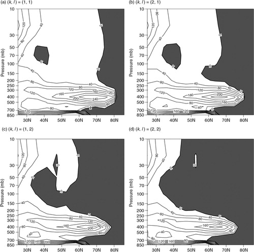
The vertical components of refractive indices (m ²) for stationary planetary waves (k, l)=(1–2, 1–2) based on winter (DJF) climatological zonal mean zonal wind is shown in Fig. 9. Areas of negative m ² correspond to the regions where waves cannot propagate. When the meridional wavenumber is equal to 2, corresponding to meridional dipole, m ² in the stratosphere shows negative values in a large part of the extratropics, particularly for (k, l)=(2, 2). This indicates that the stratospheric basic flow is unfavourable for latitudinally propagating waves. In contrast, m ² in the troposphere is dominated by large positive values in most extratropical regions, suggesting that the tropospheric basic flow is much more favourable for meridional wave propagation. Due to the constraint on meridional wavenumbers of the stratospheric basic state, waves with relatively large meridional wavenumbers may be primarily confined in the troposphere and may not be able to propagate upward into the stratosphere.

Fig. 9 (a) The vertical component of refractive index (m ²) for (k, l)=(1, 1) based on the DJF-mean zonal mean basic state in the NH. The index is scaled by a ²/10⁴. (b)–(d) as in (a), but for (k, l)=(2, 1), (k, l)=(1, 2), and (k, l)=(2, 2), respectively. In all the plots, regions with negative values are shaded.

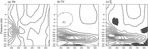
We further separate into two terms with respect to its formula; one is related to the meridional structure of the basic state , while the other is related to the vertical curvature of the basic state . These two terms are referred to as TM and TV, respectively. Figure 10 displays TM, TV and based on the DJF zonal mean basic state. The TM (Fig. 10a) shows positive values over most NH extratropical regions, with similar orders of magnitude for both the stratosphere and troposphere. However, a remarkable difference in the TV can be clearly observed between the NH stratosphere and troposphere (Fig. 10b). In the stratosphere, negative TV values prevail in the NH extratropics, most pronounced in the mid-latitude region, while the NH troposphere is mainly dominated by large positive TV values. Thus, as a result, in the stratosphere is much smaller than that in the troposphere (Fig. 10c). In addition, the magnitudes of in the stratosphere and troposphere are comparable; for example, the mean at 50 hPa is 12 m s⁻¹, while that at 500 hPa is 11 m s⁻¹. Thus, consistent with , the term is small in the stratosphere but much larger in the troposphere, and consequently, m ² is small and even negative for large meridional wavenumbers in the stratosphere. Previous theoretical studies focused on the case in which is independent of height and pointed out that the magnitude of may influence the wave propagation in the stratosphere and that waves are deflected away from those regions where is too strong (Andrews et al., 1987), but the effect of the basic state vertical curvature has not been well addressed. Therefore, the above analysis provides theoretical evidence that the vertical curvature of basic state is also an important factor that limits meridional wave propagation in the stratosphere.

Fig. 10 (a) TM, (b) TV and (c) based on the DJF-mean zonal mean basic state in the NH extratropics. For the definitions and formulas of TM, TV and , see details in the text, and all of them are scaled by a ²/10 in the plots. In (c), regions with negative values are shaded.

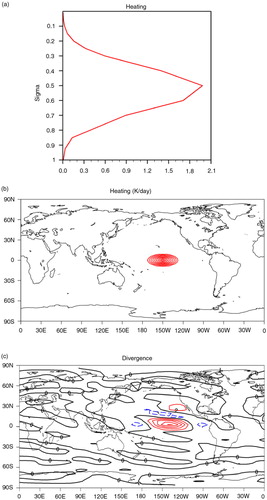
In order to further identify the role of the vertical curvature of basic state in the stratosphere, two experiments were carried out with an identical heat source imposed on the LBM (heating) as well as the one-level barotropic model (divergence). One experiment (Exp1) used the LBM that was linearised about the observed DJF zonal mean basic state. The vertical and horizontal distributions of the heating are shown in Fig. 11. The heating was centred on (0°, 150°W) with the maximum heating rate of 2 K d⁻¹ at the sigma level of 0.5. This prescribed heating was similar to the diabatic heating associated with El Niño events (Nigam et al., 2000) and the idealised heating fields used in previous LBM modelling studies (Jin and Hoskins, 1995; Ting, 1996). The other experiment (Exp2) used the barotropic model, and the zonally symmetric basic state was taken from different vertical levels between 50 and 500 hPa. The barotropic model was forced by the tropical divergence that corresponds to the heating in Exp1. As shown in Fig. 11c, the divergence was taken from the outflow level (near 200 hPa) in the LBM, regardless of the level of basic states used. This is because that the forcing in the barotropic model comes from the heating induced divergence, which is primarily confined to the heated region at the outflow level (Ting, 1996). Thus, in all the barotropic experiments, the divergence forcing was fixed at the upper-tropospheric value as shown in Fig. 11c. The wave responses from Exp1 and Exp2 were compared with each other and the effect of the basic state vertical curvature was examined.

Fig. 11 (a) Vertical and (b) horizontal distributions of the tropical heating used in Exp1. Contour interval in (b) is 0.1° K d⁻¹. (c) Divergence at 200 hPa (in 10⁻⁷ s⁻¹) computed from the steady LBM response to the tropical heating in (a) and (b).

Figure 12 shows the steady responses to the prescribed heating in Exp1. The wave response in the stratosphere (sigma level equivalent to 50 hPa, Fig. 12a) clearly exhibits a zonal wave 1 pattern, most pronounced in the western hemisphere, and does not show latitudinal wave-like structures (the spatial correlation with the S-EOF2 pattern of Fig. 5b is 0.73). In the troposphere (sigma level equivalent to 500 hPa, Fig. 12b), the wave response behaves like a meridional Rossby wave train extending from the tropical Pacific to North America and Europe (the spatial correlation with the T-EOF1 pattern of Fig. 7a is 0.64). Thus, Exp1 simulated wave responses in both the NH stratosphere and troposphere in a way that closely resemble the observed patterns of planetary waves associated with the ENSO (S-EOF2 and T-EOF1), indicating the difference in the meridional structure between planetary waves in the stratosphere and troposphere can be well captured in the LBM linearised about the observed basic state.

Fig. 12 The LBM simulated (a) stratospheric (sigma level equivalent to 50 hPa) and (b) tropospheric (sigma level equivalent to 500 hPa) responses of eddy geopotential height (in m) to the prescribed heating in Fig. 11. Linear barotropic model responses in eddy geopotential height (in m) to the tropical divergence forcing of Fig. 11c when linearised about the zonal mean flow at (c) 50 hPa and (d) 500 hPa. In all the barotropic experiments, the geopotential height was obtained by multiplying the streamfunction by the Coriolis parameter.

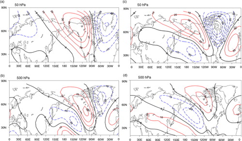
In Exp2, the effect of the basic state vertical curvature is absent, and the wave response in the stratosphere (Fig. 12c) is completely different from that in Exp1. It looks like the meridional Rossby wave train in the troposphere (Fig. 12b) but with stronger amplitudes and a broader spatial extent, and clearly shows latitudinal wave-like structures in the North Pacific and North Atlantic regions. The tropospheric wave response in Exp2 (Fig. 12d) is similar to that in Exp1, both showing a meridional wave train pattern. Thus, by comparing the simulation results in Exp1 and Exp2, we may conclude that the vertical curvature of the stratospheric zonal mean basic state strongly limits the meridional wave propagation, in consistence with the theoretical analysis.

6. Summary and discussion

Based on the spherical DFS expansion of geopotential height data, the horizontal structures of NH stratospheric and tropospheric PWV were investigated and compared in the 2D wavenumber space. Comparing the amplitudes of wave components during the last three decades, the results suggest that PWV in the troposphere significantly differs from those in the stratosphere, especially in meridional structure. In particular, eddy geopotential height anomalies in the stratosphere are dominated by large-scale zonal wave patterns, particularly zonal waves 1 and 2. These patterns have little latitudinal wave-like fluctuation and are most pronounced during the cold season. In contrast, PWV in the NH troposphere mainly exhibits 2D Rossby wave patterns in the wavenumber space and show latitudinal wave-like fluctuations, corresponding to the Rossby wave dispersion in the meridional direction on the sphere. The meridional dipole in the tropospheric eddy geopotential height is most prominent during the cold season; while during the warm season, the dominant meridional scale may become smaller.

The first two EOFs of the winter stratospheric eddy geopotential height (S-EOF1 and S-EOF2), which were shown to be related to QBO and ENSO variations, respectively, are both characterised by the large-scale zonal wave 1 pattern, further confirming the leading role of zonal wave 1 pattern. In contrast, both the leading two EOFs of the winter tropospheric eddy geopotential height (T-EOF1 and T-EOF2) are dominated by meridional dipoles, as indicated in the 2D wavenumber space. It was also found that the ENSO and NAO signals may account for the variability of the T-EOF1 and T-EOF2 patterns, respectively.

Theoretical and modelling analyses were then conducted to qualitatively interpret the observational findings. It was found that the tropospheric basic state is much more favourable for latitudinally propagating stationary waves than the stratospheric basic state. The difference can also be realistically simulated in a LBM with the observed zonal mean basic state. Furthermore, both theoretical and modelling results suggested that the fact that zonal wave patterns are preferred in the NH stratosphere can be partly attributed to the vertical curvature of the stratospheric zonal mean basic state.

The present work focused on the difference in the horizontal structure between NH stratospheric and tropospheric PWV; however, we do not rule out a possible relationship between them. Previous studies have demonstrated a strong connection between stratospheric and tropospheric planetary waves (Perlwitz and Graf, 1995, 2001; Garfinkel and Hartmann, 2007, 2008). Thus, further analyses are required to investigate how to depict this connection in the 2D wavenumber space and to determine what structures of planetary waves are most active in the interaction between the stratosphere and troposphere. The spherical DFS method also provides a useful tool for further evaluating the relative roles of planetary waves with different meridional structures in the wave–mean-flow interaction (Ting et al., 1996; DeWeaver and Nigam, 2000; Kimoto et al., 2001). In addition, the theoretical interpretation in the present study is preliminary and qualitative, and there is a lack of analysis of detailed physical processes related to the observed meridional structures of PWV. For example, the dominant role of the meridional dipole structure in the troposphere may be attributable to other complicated processes, such as synoptic eddy and low-frequency flow feedback (Jin et al., 2006; Kug and Jin, 2009). Moreover, the authors plan to extend the analyses in the present work to the Southern Hemisphere and to explore the possible difference between the two hemispheres.

Acknowledgements

The authors wish to thank the anonymous reviewers for their constructive comments that contributed to improve this paper. This work was jointly supported by the NSFC Projects 41305046 and 41290255, and the Climate Change Special Project of the State Ocean Administration.

References

- Andrews D. G. , Holton J. R. , Leovy C. B . Middle Atmospheric Dynamics. 1987; , New York 489. Academic Press.
- Athanasiadis P. J. , Ambaum M. H. P . Linear contributions of different time scales to teleconnectivity. J. Clim. 2009; 22(13): 3720–3728.
- Barnston A. G. , Livezey R. E . Classification, seasonality and persistence of low-frequency atmospheric circulation patterns. Mon. Wea. Rev. 1987; 115: 1083–1126.
- Blackmon M. L. , Madden R. A. , Wallace J. M. , Gutzler D. S . Geographical variations in the vertical structure of geopotential height fluctuations. J. Atmos. Sci. 1979; 36(12): 2450–2466.
- Blackmon M. L. , Lee Y. H. , Wallace J. M . Horizontal structure of 500-mb height fluctuations with long, intermediate and short-time scales. J. Atmos. Sci. 1984; 41(6): 961–979.
- Boer G. J. , Fourest S. , Yu B . The signature of the annular modes in the moisture budget. J. Clim. 2001; 14(17): 3655–3665.
- Charney J. G. , Drazin P. G . Propagation of planetary-scale disturbances from lower into upper atmosphere. J. Geophys. Res. 1961; 66(1): 83–109.
- Chen W. , Huang R. H . The propagation and transport effect of planetary waves in the Northern Hemisphere winter. Adv. Atmos. Sci. 2002; 19(6): 1113–1126.
- Chen W. , Takahashi M. , Graf H. F . Interannual variations of stationary planetary wave activity in the northern winter troposphere and stratosphere and their relations to NAM and SST. J. Geophys. Res. 2003; 108: 4797.
- Chen W. , Yang S. , Huang R. H . Relationship between stationary planetary wave activity and the East Asian winter monsoon. J. Geophys. Res. 2005; 110(D14): 14110.
- Cheong H. B. , Kwon I. H. , Goo T. Y . Further study on the high-order double-Fourier-series spectral filtering on a sphere. J. Comput. Phys. 2004; 193(1): 180–197.
- DeWeaver E. , Nigam S . Zonal-eddy dynamics of the North Atlantic oscillation. J. Clim. 2000; 13(22): 3893–3914.
- Edmon H. J. , Hoskins B. J. , Mcintyre M. E . Eliassen-Palm cross-sections for the troposphere. J. Atmos. Sci. 1980; 37(12): 2600–2616.
- Folland C. K. , Knight J. , Linderholm H. W. , Fereday D. , Ineson S. , co-authors . The summer North Atlantic Oscillation: past, present, and future. J. Clim. 2009; 22(5): 1082–1103.
- Garcia-Herrera R. , Calvo N. , Garcia R. R. , Giorgetta M. A . Propagation of ENSO temperature signals into the middle atmosphere: a comparison of two general circulation models and ERA-40 reanalysis data. J. Geophys. Res. 2006; 111(D6): 06101.
- Garfinkel C. I. , Hartmann D. L . Effects of the El Nino-Southern Oscillation and the Quasi-Biennial Oscillation on polar temperatures in the stratosphere. J. Geophys. Res. 2007; 112(D19): 19112.
- Garfinkel C. I. , Hartmann D. L . Different ENSO teleconnections and their effects on the stratospheric polar vortex. J. Geophys. Res. 2008; 113(D18): 18114.
- Garfinkel C. I. , Shaw T. A. , Hartmann D. L. , Waugh D. W . Does the Holton-Tan mechanism explain how the quasi-biennial oscillation modulates the arctic polar vortex?. J. Atmos. Sci. 2012; 69(5): 1713–1733.
- Hannachi A . On the origin of planetary-scale extratropical winter circulation regimes. J. Atmos. Sci. 2010; 67(5): 1382–1401.
- Harnik N. , Lindzen R. S . The effect of reflecting surfaces on the vertical structure and variability of stratospheric planetary waves. J. Atmos. Sci. 2001; 58(19): 2872–2894.
- Held I. M. , Ting M. F. , Wang H. L . Northern winter stationary waves: theory and modelling. J. Clim. 2002; 15(16): 2125–2144.
- Holton J. R. , Tan H. C . The influence of the equatorial quasi-biennial oscillation on the global circulation at 50 Mb. J. Atmos. Sci. 1980; 37(10): 2200–2208.
- Hoskins B. J. , Karoly D. J . The steady linear response of a spherical atmosphere to thermal and orographic forcing. J. Atmos. Sci. 1981; 38(6): 1179–1196.
- Hu Y. Y. , Tung K. K . Interannual and decadal variations of planetary wave activity, stratospheric cooling, and Northern Hemisphere Annular mode. J. Clim. 2002; 15(13): 1659–1673.
- Hurrell J. W . Decadal trends in the North-Atlantic Oscillation-regional temperatures and precipitation. Science. 1995; 269(5224): 676–679.
- Ineson S. , Scaife A. A . The role of the stratosphere in the European climate response to El Nino. Nat. Geosci. 2009; 2(1): 32–36.
- Jin F. F. , Hoskins B. J . The direct response to tropical heating in a baroclinic atmosphere. J. Atmos. Sci. 1995; 52(3): 307–319.
- Jin F. F. , Pan L. L. , Watanabe M . Dynamics of synoptic eddy and low-frequency flow interaction. Part I: a linear closure. J. Atmos. Sci. 2006; 63(7): 1677–1694.
- Kalnay E. , Kanamitsu M. , Kistler R. , Collins W. , Deaven D. , co-authors . The NCEP/NCAR 40-year reanalysis project. Bull. Am. Meteorol. Soc. 1996; 77(3): 437–471.
- Kanamitsu M. , Ebisuzaki W. , Woollen J. , Yang S. K. , Hnilo J. J. , co-authors . NCEP-DOE AMIP-II reanalysis (R-2). Bull. Am. Meteorol. Soc. 2002; 83(11): 1631–1643.
- Kaplan A. , Cane M. A. , Kushnir Y. , Clement A. C. , Blumenthal M. B. , co-authors . Analyses of global sea surface temperature 1856–1991. J. Geophys. Res. 1998; 103(C9): 18567–18589.
- Karoly D. J . Southern Hemisphere circulation features associated with El nino-Southern Oscillation events. J. Clim. 1989; 2(11): 1239–1252.
- Kimoto M. , Jin F. F. , Watanabe M. , Yasutomi N . Zonal-eddy coupling and a neutral mode theory for the Arctic Oscillation. Geophys. Res. Lett. 2001; 28(4): 737–740.
- Kug J.-S. , Jin F.-F . Left-hand rule for synoptic eddy feedback on low-frequency flow. Geophys. Res. Lett. 2009; 36(5): 05709.
- Kuo H. L . On quasi-nondivergent prognostic equations and their integration. Tellus. 1956; 8(3): 373–383.
- Layton A. T. , Spotz W. F . A semi-Lagrangian double Fourier method for the shallow water equations on the sphere. J. Comput. Phys. 2003; 189(1): 180–196.
- Li J. P. , Sun C. , Jin F. F . NAO implicated as a predictor of Northern Hemisphere mean temperature multidecadal variability. Geophys. Res. Lett. 2013; 40(20): 5497–5502.
- Li J. P. , Wang J. X. L . A new North Atlantic Oscillation index and its variability. Adv. Atmos. Sci. 2003; 20(5): 661–676.
- Li Q. , Graf H. F. , Giorgetta M. A . Stationary planetary wave propagation in Northern Hemisphere winter – climatological analysis of the refractive index. Atmos. Chem. Phys. 2007; 7: 183–200.
- Manzini E. , Giorgetta M. A. , Esch M. , Kornblueh L. , Roeckner E . The influence of sea surface temperatures on the northern winter stratosphere: ensemble simulations with the MAECHAM5 model. J. Clim. 2006; 19(16): 3863–3881.
- Matsuno T . Vertical propagation of stationary planetary waves in winter Northern Hemisphere. J. Atmos. Sci. 1970; 27(6): 871–883.
- Nigam S. , Chung C. , DeWeaver E . ENSO diabatic heating in ECMWF and NCEP-NCAR reanalyses, and NCAR CCM3 simulation. J. Clim. 2000; 13(17): 3152–3171.
- Nigam S. , Lindzen R. S . The sensitivity of stationary waves to variations in the basic state zonal flow. J. Atmos. Sci. 1989; 46(12): 1746–1768.
- North G. R. , Bell T. L. , Cahalan R. F. , Moeng F. J . Sampling errors in the estimation of empirical orthogonal functions. Mon. Weather Rev. 1982a; 110(7): 699–706.
- North G. R. , Moeng F. J. , Bell T. L. , Cahalan R. F . The latitude dependence of the variance of zonally averaged quantities. Mon. Weather Rev. 1982b; 110(5): 319–326.
- Ogi M . The summertime annular mode in the Northern Hemisphere and its linkage to the winter mode. J. Geophys. Res. 2004; 109(D20): 20114.
- Perlwitz J. , Graf H. F . The statistical connection between tropospheric and stratospheric circulation of the northern-hemisphere in winter. J. Clim. 1995; 8(10): 2281–2295.
- Perlwitz J. , Graf H. F . The variability of the horizontal circulation in the troposphere and stratosphere – a comparison. Theor. Appl. Climatol. 2001; 69(3–4): 149–161.
- Perlwitz J. , Harnik N . Observational evidence of a stratospheric influence on the troposphere by planetary wave reflection. J. Clim. 2003; 16(18): 3011–3026.
- Pyper B. J. , Peterman R. M . Comparison of methods to account for autocorrelation in correlation analyses of fish data. Can. J. Fish. Aquat. Sci. 1998; 55: 2127–2140.
- Randel W. J. , Wu F. , Stolarski R . Changes in column ozone correlated with the stratospheric EP flux. J. Meteorol. Soc. Jpn. 2002; 80(4B): 849–862.
- Rossby C. G . Relation between variations in the intensity of the zonal circulation of the atmosphere and the displacements of the semipermanent centres of action. J. Mar. Res. 1939; 2(1): 38–55.
- Simmons A. , Uppala S. , Dee D. , Kobayashi S . ERA–Interim: new ECMWF reanalysis products from 1989 onwards. ECMWF Newslett. 2007; 110: 25–35.
- Simmons A. J. , Wallace J. M. , Branstator G. W . Barotropic wave-propagation and instability, and atmospheric teleconnection patterns. J. Atmos. Sci. 1983; 40(6): 1363–1392.
- Sun C. , Li J. P . Space-time spectral analysis of the southern hemisphere daily 500-hpa geopotential height. Mon. Weather Rev. 2012; 140(12): 3844–3856.
- Sun C. , Li J. P. , Jin F. F. , Ding R. Q . Sea surface temperature inter-hemispheric dipole and its relation to tropical precipitation. Environ. Res. Lett. 2013; 8: 044006.
- Thompson D. W. J. , Wallace J. M . Annular modes in the extratropical circulation. Part I: month-to-month variability. J. Clim. 2000; 13(5): 1000–1016.
- Ting M. F . Steady linear response to tropical heating in barotropic and baroclinic models. J. Atmos. Sci. 1996; 53(12): 1698–1709.
- Ting M. F. , Hoerling M. P. , Xu T. Y. , Kumar A . Northern hemisphere teleconnection patterns during extreme phases of the zonal-mean circulation. J. Clim. 1996; 9(10): 2614–2633.
- Trenberth K. E. , Branstator G. W. , Karoly D. , Kumar A. , Lau N. C. , co-authors . Progress during TOGA in understanding and modelling global teleconnections associated with tropical sea surface temperatures. J. Geophys. Res. 1998; 103(C7): 14291–14324.
- van Loon H. , Labitzke K . The Southern Oscillation: the anomalies in the lower stratosphere of the Northern-Hemisphere in winter and a comparison with the quasi-biennial oscillation. Mon. Weather Rev. 1987; 115(2): 357–369.
- Wallace J. M . North Atlantic Oscillation/annular mode: two paradigms – one phenomenon. Q. J. Roy. Meteorol. Soc. 2000; 126(564): 791–805.
- Wallace J. M. , Blackmon M. L . Hoskins B. , Pearce R . Observations of low-frequency atmospheric variability. I Large-scale dynamical processes in the atmosphere. 1983; San Diego, California, Academic Press. 55–94.
- Wallace J. M. , Gutzler D. S . Teleconnections in the geopotential height field during the northern hemisphere winter. Mon. Weather Rev. 1981; 109(4): 784–812.
- Wang L. , Huang R. H. , Gu L. , Chen W. , Kang L. H . Interdecadal variations of the East Asian winter monsoon and their association with quasi-stationary planetary wave activity. J. Clim. 2009; 22(18): 4860–4872.
- Watanabe M . Asian jet waveguide and a downstream extension of the North Atlantic Oscillation. J. Clim. 2004; 17(24): 4674–4691.
- Watanabe M. , Kimoto M . Atmosphere-ocean thermal coupling in the North Atlantic: a positive feedback. Q. J. Roy. Meteorol. Soc. 2000; 126(570): 3343–3369.
- Wei K. , Chen W. , Huang R. H . Association of tropical Pacific sea surface temperatures with the stratospheric Holton-Tan Oscillation in the Northern Hemisphere winter. Geophys. Res. Lett. 2007; 34(16): 16814.
- Xie F. , Li J. , Tian W. , Feng J. , Huo Y . Signals of El Nino Modoki in the tropical tropopause layer and stratosphere. Atmos. Chem. Phys. 2012; 12(11): 5259–5273.
- Wu Z. W. , Wang B. , Li J. P. , Jin F. F . An empirical seasonal prediction model of the East Asian summer monsoon using ENSO and NAO. J. Geophys. Res. 2009; 114: 18120.
- Wu Z. W. , Li J. P. , Jiang Z. H. , He J. H. , Zhu X. Y . Possible effects of the North Atlantic Oscillation on the strengthening relationship between the East Asian Summer monsoon and ENSO. Int. J. Climatol. 2012; 32(5): 794–800.
- Yeh T. C . On energy dispersion in the atmosphere. J. Meteorol. 1949; 6(1): 1–16.
- Zuo J. Q. , Li W. J. , Sun C. H. , Xu L. , Ren H. L . Impact of the North Atlantic sea surface temperature tripole on the East Asian summer monsoon. Adv. Atmos. Sci. 2013; 30(4): 1173–1186.