The impact of assimilating data from a remotely piloted aircraft on simulations of weak-wind orographic flow

Abstract

Orographic winds near a 914 m high mountain in Southwest-Iceland are explored using unique observations made aloft with a small remotely piloted aircraft, as well as with traditional observations and high-resolution atmospheric simulations. There was an inversion well above mountain top level at about 2 km with weak winds below. Observed winds in the lee of the mountain were indicative of flow locally enhanced by wave activity aloft. Winds descended along the lee slope with a prevailing direction away from the mountain. They were relatively strong and gusty at the surface close to the mountain, with a maximum at low levels, and weakening and becoming more diffuse a short distance further downstream. The winds weakened further aloft, with a minimum on average near mountain top level. This situation is reproduced in a high-resolution atmospheric simulation forced with atmospheric analysis as well as with the observed lee-side profiles of wind and temperature below 1.4 km. Without the additional observations consisting of the lee-side profiles, the model fails to reproduce the winds aloft as well as at the surface in a region in the lee of the mountain, as was also the case for the operational numerical models at that time. A sensitivity simulation indicates that this poor performance is a result of the poorly captured strength and sharpness of the inversion aloft. The study illustrates, firstly, that even at very low wind speed, in a close to neutral low-level flow, gravity waves may still be a dominating feature of the flow. Secondly, the study presents an example of the usefulness of lee-side atmospheric profiles, retrieved by simple model aircraft, for improving numerical simulations and short-term weather forecasting in the vicinity of mountains. Thirdly, the study confirms the sensitivity of downslope flow to only moderate change in the sharpness of an upstream inversion.

• downslope flow
• complex orography
• small remotely piloted aircraft
• observational nudging

1. Introduction

The relatively recent improvement in atmospheric simulations of mesoscale and small-scale mountain weather is the cumulative result of several important factors, some of which are the higher spatial resolution, made available by increasing computing power; the improvements made to the parameterizations of physical and dynamical processes related to, for example, atmospheric water, radiation and fluxes (e.g. Teixeira et al., 2008; Gilliam and Pleim, 2010; Hu et al., 2013) and the more numerous and accurate atmospheric observations available for preparing global atmospheric analyses and feeding-improved assimilation systems (e.g. Langland et al., 1999; Alapaty et al., 2001; de Rosnay et al., 2014).

Successful numerical simulations of local weather in complex topography are dependent on the model resolution being sufficient for resolving the dominating topography; both when downscaling the wind climate as well as when simulating extreme wind events in complex terrain (e.g. Ágústsson and Ólafsson, 2007; Horvath et al., 2012; Jonassen et al., 2013), but also for capturing middle and upper level tropospheric flow above complex terrain (e.g. Doyle et al., 2005; Ólafsson and Ágústsson, 2009). Operational systems are aiming at a horizontal resolution of 1 km or better, and research models have long reached this resolution. Part of the work on the parameterisation schemes goes into improving the methods for describing physics and dynamics which may have been adequately accurate at coarser resolutions, but may not be applicable in the push towards higher sub-kilometre resolutions (e.g. Wyngaard, 2004; Horvath et al., 2012).

Another decisive factor for successful simulations of the weather is the quality of the atmospheric data used to initialise and force the models at their boundaries. This data often originates from global atmospheric re-analysis, operational analysis or forecasts at relatively coarse resolutions, typically 15–80 km in the horizontal, with a temporal resolution of 1–6 hours. Frequently, the accuracy and resolution of this data is not adequate for high-resolution simulations of local and small-scale features which may be dependent on small deviations in the large-scale flow, as pointed out by Reinecke and Durran (2009) in their study of gravity wave activity above complex orography. In spite of the global coverage of the remote sensing data, which has significantly improved atmospheric analyses, such analyses may suffer in otherwise data-sparse and mountainous regions of the world. For such cases, the initial and forcing data can be supplemented and improved by assimilating additional in-situ or remote sensing observations (Schroeder et al. 2006; Stauffer and Seaman 1990, 1994).

One recent study that employs observational nudging to improve high-resolution simulations is that of Jonassen et al. (2012), who studied the sea breeze during the MOSO-project in Southwest-Iceland (named after the small town Mosfellsbær near Reykjavík). The novel observations used as additional model forcing were made aloft with a small unmanned meteorological observer (SUMO), also referred to as a remotely piloted aircraft system (RPAS, Reuder et al., 2009), described further in the next section. Here, we analyse observations from the MOSO-project, made with the RPAS on 15 July 2009 in the lee of Mt. Esja in Southwest-Iceland. The observations reveal unexpected downslope accelerated flow in a weak-wind situation where gravity wave activity was not expected and not forecast by the operational numerical systems, even though these systems operate at high spatial resolution (1–3 km). The following section describes the study region, the observational data and the setup of the mesoscale numerical model used to simulate the atmospheric flow. Sections 3 and 4 describe the observed and simulated atmospheric flow, respectively. This is followed by an analysis of the flow and discussions on its dynamics. The paper is concluded with a short summary and remarks on the most important findings of the study.

2. Method and data

2.1. Study region

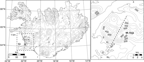
The MOSO-project had several intensive observation periods where flow near and around Mt. Esja in Southwest-Iceland was studied and analysed (Fig. 1). Mt. Esja is a prominent landmark of Reykjavík, and rises to 914 m from sea level at a distance of 10 km from the city centre. The mountain slopes are steep, and it is relatively narrow in the north–south direction (~5 km) while its length is roughly four times as great. Its westernmost tip is located at the coast while in the east it merges with other mountain massifs. In addition to being easily accessible and in a well-equipped region with regard to atmospheric observations, Mt. Esja is known to have a strong influence on weather in Reykjavík and in the surrounding region. There is, for example, often an extended wake of weak winds in the lee of the mountain sheltering all, or parts, of Reykjavík, depending on wind direction and speed aloft. Traffic is often disrupted by frequent downslope windstorms at the foot of the mountain, some of which reach as far as Reykjavík.

Fig. 1 Model topography (left, 200 m contours) at 3 km resolution, and in the main region of interest (Z) within the 1-km resolution domain (right, 100 m contours). The locations of RPAS flights (1, 2 and 3), the pseudo temperature sounding used in the sensitivity test (4), a section across Mt. Esja (dashed line), and stations at Keflavík (Ke), Reykjavík (R), Geldinganes (G), Korpa (Ko), Álfsnes (A), Kjalarnes (Kj) and Skrauthólar (S) are shown.

2.2. Observational data

On 15 July 2009, the flow aloft in the wake of Mt. Esja was explored with RPAS, which is a small, remotely piloted, aircraft system, capable of observing profiles of temperature, humidity and winds in the lower 3–4 km of the atmosphere. A detailed description of the system is given in Reuder et al. (2009), who also report on tests of the system in the Arctic near Svalbard, also presented in Mayer et al. (2012a). Prior to the MOSO-project, the RPAS was tested extensively in Iceland during the FLOHOF-experiment (Flow over and around Hofsjökull) at the Hofsjökull ice cap in the central Icelandic highlands (Reuder et al., 2012). Data from its use in Iceland have previously been presented in Mayer et al. (FLOHOF experiment, 2012b); Reuder et al. (FLOHOF-experiment, 2012), Jonassen et al. (2012, MOSO-project) and Jonassen et al. (2014, analysis of flow over the Hofsjökull ice cap). In the current study, seven RPAS flights are analysed. They are performed at three different locations to the south of the mountain (locations 1, 2 and 3 in Fig. 1), during approximately 3 hours around noon on 15 July 2009. The first flight was at 1119 UTC at location 2, with three more flights at: 1147, 1257 and 1418 UTC. At 1215 UTC a flight was performed at location 3 and two flights at 1327 and 1348 UTC were done at location 1.

In addition to the observed RPAS profiles, observations from a mesonet of automatic weather stations were available during the MOSO-project. These observations were used in analysing the flow in the lee of the mountain (station locations in Fig. 1), as well as for validating numerical simulations of the atmospheric flow at a large number of automatic weather stations in Iceland. Observations of 10-minute mean wind speed and wind direction at 10 m above ground, as well as 1-minute mean temperature at 2 m, are available with a temporal resolution of 10 minutes. The data from the automatic stations are stored and checked for systematic errors at Veðurstofa Íslands (VÍ, Icelandic Meteorological Office), excluding data from the Álfsnes station at Sorpa waste management, which was checked independently.

2.3. Setup of numerical simulations

To investigate the atmospheric flow in more detail and further corroborate the observed atmospheric data, the flow on 15 July 2009 is simulated with the non-hydrostatic mesoscale Advanced Research Weather Research and Forecasting model (ARW, version 3.4.1 Skamarock et al., 2008). The model is initialised and forced at its boundaries with the Interim re-analysis of the European Centre for Medium Range Weather Forecasts (ECMWF, resolution roughly 80 km). The simulations are done at a resolution of 9, 3 and 1 km, with respectively 95×90, 205×157 and 105×105 gridpoints in the two-way nested domains (locations are shown in Figs. 1 and 2). The simulations use 50 layers in the vertical, with higher resolution in the lower parts of the troposphere compared to further aloft (levels are indicated in Fig. 3). The layers are terrain following at lower levels with the lowest level at roughly 10 m, and flatten gradually towards the top of the model at 50 hPa. The model (9 km domain) is initialised at 0000 UTC and runs for 6 hours before starting the nested domains at 3 and 1 km, which are then run for 18 hours. This allows for circa 10 hours of spin-up time before the time of interest, with all model domains ending at 0000 UTC on 16 July. The boundary-layer parameterisation uses the Mellor–Yamada–Janjic (MYJ) scheme (Mellor and Yamada, 1982; Janjić, 1994, 2001) which is frequently used for both research and operational simulations. This 2.5 level scheme uses a second-moment closure for the turbulence and it is centred on the prognostic equation for the turbulence kinetic energy. The unified Noah land surface model (Chen et al., 1996) handles soil moisture and temperature in four layers, as well as heat and moisture fluxes at the surface, in plant canopies, and over ice and snow covered land, which are however not relevant in the region of interest. Longwave and shortwave radiation are parameterised by, respectively, the accurate and efficient rapid radiative transfer model (RRTM, Mlawer et al., 1997), and the relatively simple Dudhia (1989) scheme.

Fig. 2 Geopotential height at 700 hPa [m] (above) and mean sea level pressure [hPa] (below) at 1200 UTC on 15 July 2009 (ECMWF Interim re-analysis). Also shown are the same fields simulated (NO) at 9 km horizontal resolution (bold), as well as the 9 and 3 km domain limits (dashed lines).

Fig. 3 Skew-T diagram from the Keflavík upper-air station in Southwest-Iceland at 1200 UTC on 15 July 2009 (cf. Fig. 1 for location). Shown are observed (solid lines) and simulated (NO) at 1 km resolution (dashed lines) temperature and dew point [°C] as well as wind barbs (2.5 ms⁻¹ each half barb, observed to the right and simulated to the left) with temperature/dew point on the lower axis and height [hPa] on the vertical. Also indicated are the heights of some of the pressure levels as well as the height of model levels (extreme right).

As the atmospheric model fails to reproduce the situation when it is solely forced by the atmospheric analysis (control simulation NO), four additional simulations are performed; three of which are nudged with in-situ observations from the RPAS system. Simulation ALL nudges observations of wind and temperature from all the available RPAS profiles in the innermost 1 km domain. Simulation PBL is identical to ALL, but excluding temperature observations within the boundary layer. The setup of simulation ONE is like ALL except it only nudges the observed RPAS profile from 1147 UTC instead of all the profiles. The fourth simulation (KEF) is an additional sensitivity test, which is solely used to investigate the dynamics behind the failure of the non-nudged simulation. In the KEF simulation only, the temperature profile observed at 1200 UTC at the Keflavík upper-air station is transposed to a location upstream of Mt. Esja and nudged at 1100 UTC (location 4 in Fig. 1). As there is no other available upper-air data well outside of the wake of Mt. Esja, it is assumed that at least to a first degree, the temperature profile at Keflavík at 1200 UTC is characteristic for the upstream profile at Mt. Esja an hour earlier. With 10 ms⁻¹ as the approximate mean wind speed above the boundary layer, an air parcel would travel most of the distance between Keflavík and Mt. Esja in 1 hour but one must also take into account the temporal influence of the nudging which is in the model limited to 1 hour and 40 minutes before and after the nudged profile in the KEF simulation. The temporal influence of each nudged RPAS profile is limited to 40 minutes. The horizontal radius of influence of the nudging in all runs is held constant at 30 km, and the strength of the nudging is gradually decreased away from the origin, both in space as well as in time. It should be noted that no surface-based observations are nudged and that no RPAS data are available below roughly 30 m. The setup of the nudging is in other aspects similar to that described in Jonassen et al. (2012), which includes a short description of the nudging system in the ARW-model (Stauffer and Seaman, 1994) as implemented by Liu et al. (2005). The key difference between the nudging method applied here, frequently referred to as four dimensional data assimilation (FDDA) and any other available assimilation methods, is that the nudging is applied at model runtime and requires little pre-processing while most other methods require more detailed and systematic analysis to be carried out beforehand. As such, the current method is better adapted to ad-hoc nudging of available data in data-sparse regions and/or where a more detailed analysis is not feasible or possible within the given timeframe. It does however not provide a systematic method to analyse the impact of each nudged observation on the quality of the simulations.

All discussion of the synoptic-scale flow, as well as mesoscale flow away from the region of main interest, is limited to results based on the control simulation (NO). Results from the nudged runs are only shown when discussing fine scale features of local weather near Mt. Esja, in a region inside the 1 km numerical domain (region Z in Fig. 1). Results from a series of non-nudged sensitivity simulations are not presented here but they all gave similar results and failed to capture the observed flow in the lee. Namely, the case was also simulated using several other boundary layer schemes, with reduced surface roughness, using higher horizontal and vertical resolution (at low tropospheric levels, including the boundary layer) as well as with forcing data based on the operational GFS-analysis (Global Forecast System) as well as the ECMWF operational analysis on model and pressure levels.

3. Observations of the atmospheric flow

According to the Interim atmospheric re-analysis (Dee et al., 2011) from the ECMWF, there was at the time of interest low pressure between Iceland and Scotland and high pressure over Greenland (Fig. 2, thin lines). The pressure gradients were modest and consequently there was weak northeasterly flow at low levels over Iceland, as observed above the Keflavík upper-air station in Southwest-Iceland (Fig. 3), within 50 km west of the region of interest. The winds increase slowly from 5 ms⁻¹ at approximately 900 hPa to 10 ms⁻¹ at 700 hPa, with much stronger winds further aloft.

The RPAS observations reveal a profile of northeasterly downslope flow, which was unexpected as the operational models predicted a westerly breeze from the sea and into the mountain wake. All the profiles (Fig. 4, upper panel) are characterised by northerly and easterly winds, generally increasing in strength with height in the lowest few hundred metres above ground but weakening further aloft with the weakest winds on average at or above mountain top level. There is an easterly veering of the wind with height, which is most pronounced closest to the mountain. The observed wind maximum has the smallest vertical extent close to the mountain, that is, at location 3, and becomes more diffuse and weaker further away from the mountain (locations 1 and 2). As the RPAS does not give reliable data below roughly 30 m above ground, the winds at the surface at the locations of the RPAS flights were subjectively estimated from their effect on the conditions on land or sea. They were northerly at all locations, ~7 ms⁻¹ and gusty at locations 3 and 2, closest to the mountain, and weaker at location 1. There is in general a warm surface layer (>~12°C), extending up to 100–200 m. This layer is not far from being isothermal in the first observed profile and it thickens during the day. Above ~600 m, the temperature does not decrease much with height. The northerly surface winds in the region, and in particular, near the RPAS sites are verified by observations from automatic weather stations, for example, at Álfsnes (dots in Fig. 5, location A in Fig. 1). Here, the winds were northerly from approximately 1200 UTC and during the remainder of the day. The temperature increase from morning to afternoon is disrupted by three periods of decreasing temperatures. The first decrease at 1120 UTC is correlated with a short period of north-northwesterly winds from the sea while at 1210 UTC and 1430 UTC there is a correlation with significantly increased northerly winds of up to 9–10 ms⁻¹. The first period of cooling may be associated with advection of colder air while the latter two periods are expected to be a result of a burst of increased mixing of the warm surface layer with cooler air from aloft.

Fig. 4 Observed and simulated vertical profiles of winds [ms⁻¹] and temperature [°C] (bars), as well as 2-m temperature (dots) on 15 July 2009. Observed profiles (above) are from the descending part of the RPAS flights (locations indicated at top of bars and in Fig. 1), with 2-m temperature from Álfsnes. Simulated surface temperature and profiles (below) are from the NO (red arrows/right column) and ALL (green arrows/left column) 1 km domains and they are taken at/above the Álfsnes automatic weather station (Fig. 1).

Fig. 5 Observations and simulations (1 km resolution) of 10-m surface wind speed [ms⁻¹] (above) and direction [°] (centre), as well as 2-m temperature [°C] (below) at Álfsnes (location A in Fig. 1). The spread of the simulated values (ALL) in a 3×3 km² area centred on the station location is bounded within the grey envelope. The dashed, vertical, lines indicate the time interval with available RPAS observations.

4. The simulated flow

At the synoptic scale, both the mean sea level pressure and the height of the 700 hPa level on 15 July 2009 are well reproduced at the coarsest resolutions of 9 km (Fig. 2). The error (simulated-observed) in mean sea level pressure is on average within 0.2 hPa and less than 2 m in the height of the 700 hPa level. The largest discrepancies are found near the southern and eastern coastline of Iceland (0.5 hPa and 5 m) and are a result of orographically disturbed flow which is far better represented at 9 km than at the much coarser resolution of the analysis.

There are no upper-air observations available to verify the structure of the flow impinging on Mt. Esja. The only available upper-air observations are from Keflavík, which is located about 50 km to the west. The model captures to a good extent the overall structure of the atmosphere above Keflavík (Fig. 3, not corrected for the drift of the sonde), including the depth of the near neutral boundary layer. The fine-scale structures are in general not captured and the most significant discrepancy is found in the missing temperature inversion of approximately 2 K at 775 hPa. From 875 hPa and up to the inversion, the simulated profile is similarly stratified as in the observed profile. Above the inversion and up to 700 hPa the simulated stratification is stronger than what is observed while the stratification is roughly the same further aloft. Such errors in the sharpness of small-scale features of the temperature profile have previously been observed and may presumably be related to the limited vertical resolution of the model and the forcing data (Teixeira et al., 2008), as well as excessive mixing/diffusion in the boundary layer parameterisation. The winds at low levels are quite correct, but at high tropospheric levels, the wind speed error is up to 10 ms⁻¹ as the simulated forward wind shear is too weak. Humidity is slightly overestimated at middle and upper tropospheric levels, and its layering is not captured, but it is reasonably well captured at lower levels. Such errors in the layering of simulated humidity may be attributed to either insufficient vertical resolution of the atmospheric model and the forcing data as in Rögnvaldsson et al. (2007) or to complications in measuring humidity.

The flow simulated at 3 km (NO) reveals that the large-scale flow is strongly affected by the complex orography of Iceland (Fig. 6). There is speed-up in corner winds in the northwest and at the southeast coast, as well as on the lee slopes of many large mountains. Weak winds are observed and simulated in an upstream blocking at the north coast and in Northeast Iceland as well as in a wake covering large parts of South Iceland. There is considerably more detail in the surface flow in Southwest-Iceland when simulated at 1 km than at 3 km (cf. Fig. 6 and Fig. 7). The increase in detail is, however, not as great as when going from 9 to 3 km (not shown).

Fig. 6 Simulated 10-m wind speed [ms⁻¹] and wind vectors at a horizontal resolution of 3 km (NO), as well as observed 10-m winds at automatic weather stations (numbers and barbs, 2.5 ms⁻¹ each half barb), at 1200 UTC on 15 July 2009.

Fig. 7 Simulated 10-m wind speed [ms⁻¹] and wind vectors at a horizontal resolution of 1 km (NO), as well as observed 10-m winds at automatic weather stations (numbers and barbs, 2.5 ms⁻¹ each half barb), at 1200 UTC on 15 July 2009.

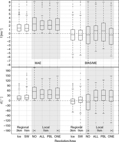
The observed winds are on average well reproduced at 33 automatic weather stations located throughout Iceland in the 3 km domain, as well as at 20 stations in the 1 km domain in Southwest-Iceland, as indicated by the statistics summarised in Fig. 8. Note that most of the stations in the main region of interest near Mt. Esja are excluded from this comparison (those depicted in Fig. 1), and that not all of the stations employed at 1 km (20 stations) can be adequately represented at 3 km. There is a general improvement in the model performance in Southwest-Iceland when the horizontal resolution is increased from 3 to 1 km, but this improvement is not well reflected in Fig. 8 (regional). At 1 km in Southwest-Iceland (and at 3 km throughout Iceland), winds are on average underestimated by 0.3 ms⁻¹ with a mean absolute error of 1.5 ms⁻¹ or less at half of the locations. The mean error at individual stations ranges between −5 and 5 ms⁻¹, with the errors in the range of −2–1 ms⁻¹ at more than half of the stations. The bias in wind direction is mostly between −60 and 60° and the mean absolute error is less than 30° at 3/4 of the stations, but is in general slightly greater at 1 km than at 3 km. Most of the significant errors in wind speed and wind direction are found at locations where the observed flow is relatively weak and variable, and/or at locations where sub-grid orography is of importance. An investigation of the simulated wind field reveals that the errors at these sites can often be explained by the large spatial and temporal variability of the simulated winds (not shown). Observed temperatures are captured with an absolute error of 1.5°C or less and a bias no greater than 1°C at most of the stations (not shown).

Fig. 8 Mean absolute error (MAE) and mean error (BIAS/ME) for simulated wind speed (above) and direction (below). The regional flow in Iceland (Ice, 3 km) and Southwest-Iceland (SW, 1 km) is presented based on the NO simulation. The local flow in the main region of interest is presented for five stations (Fig. 1; S, Kj, A, G and Ko) and the NO, ALL, PBL and ONE 1 km simulations (shaded region). The median is given by the horizontal line inside the box which covers the 25% and 75% quartiles, while whiskers show the range of the data, excluding outliers.

There is a clear change in the character of the flow in the main region of interest (Fig. 9), that is, in the lee of Mt. Esja, when the atmospheric model is either nudged with observations from the RPAS (ALL, PBL, ONE) or with the upstream temperature profile (KEF), compared to a non-nudged simulation (NO). Without the nudging, the atmospheric model fails to predict the northerly, strong and gusty flow observed at Álfsnes. Instead, it predicts a pattern reminiscent of a sea breeze, with cool and weak westerly flow directed onshore and into the wake of Mt. Esja (cf. Fig. 5). From visual inspection of the observed and simulated surface wind and temperature fields, it is evident that the effect of the nudging is limited both in time and space (Fig. 7 and similarly for the nudged simulations not shown here, as well as Figs. 5, 9 and 10). The impact of the nudging is strongest at the origin, but while the model limits the horizontal radius of influence of each nudged profile to 30 km, there is effectively little influence beyond 20 km. Finally, roughly 2 hours after the last nudged RPAS profile, the effect of the nudging is more or less lost at the stations in the region of interest. The nudged simulations all reproduce flow with a similar character as the observed flow, that is, northerly or easterly flow directed away from Mt. Esja. There is an improvement in the mean absolute error (less spread and lower median of the error), and to some degree in the bias (less spread of the error), for all nudged runs when compared to the control run (Fig. 8). However, the performance of the nudged simulations varies considerably between the five stations for which the statistics are investigated. As expected, there is somewhat better performance near the RPAS site than at more distant stations. The temperature is well captured at Álfsnes (Fig. 5), in the morning and the evening as well as during the nudging period when the errors are on average considerably smaller than 1°C. The greatest error (>2°C) in temperature is found in the afternoon after 1500 UTC, when a 2°C decrease in temperature is associated with an ~2 ms⁻¹ increase in wind speed. The wind direction is best reproduced in the PBL simulation where the errors are less than 45° during the nudging period. The weak winds in the morning and late afternoon are not captured and neither are the observed wind maxima at 1300 and 1500 UTC. The greatest improvement in simulated wind direction (Fig. 10) as well as in temperature and wind speed (not shown) is seen for the ALL and PBL simulation at Kjalarnes which is located at the foot of Mt. Esja. Here, the wind speed and wind direction are reasonably well captured. At Skrauthólar, also at the foot of Mt. Esja, it is not clear which nudging setup is best. Temperature is well captured with the PBL simulation at Korpa (about 6 km downstream of Mt. Esja), while the ONE simulation is on average best for simulated winds. At Reykjavík, a station well outside of the immediate lee of the mountain, the ONE simulation is best for capturing the wind direction while ALL is best for both wind speed and temperature. Here, the largest errors in wind speed (3 ms⁻¹) and temperature (up to 2°C) occur in the late afternoon, approximately 1.5 hours after the last RPAS profile. The simulations fail to capture the sudden change in the observed wind direction in the evening and show instead a gradual turning of the wind, starting in the afternoon.

Fig. 9 Simulated 10-m wind speed [ms⁻¹] and wind vectors at a horizontal resolution of 1 km in the NO (upper left), ALL (right) and KEF (below) simulations, as well as observed 10-m winds at automatic weather stations (numbers and barbs, 2.5 ms⁻¹ each half barb), at 1400 UTC on 15 July 2009. Terrain contours with 100 m interval.

Fig. 10 Observed and simulated 10-m wind direction [°] at four automatic weather stations on 15 July 2009. Simulated values are from the 1 km horizontal domain for the control run (NO) and three nudged runs. The spread of the simulated values (ALL) in a 3×3 km² area centred on the station location is bounded within the grey envelope. The dashed, vertical, lines indicate the time interval with available RPAS observations.

The section across Mt. Esja (Fig. 11), as well as the profiles in the lee of the mountain (Fig. 4, lower panel), show that the flow in the lee of Mt. Esja is in two different states in the NO and ALL/KEF simulations. Without nudging, there is shallow and weak westerly flow south of the mountain, reminiscent of a sea breeze; a situation not observed in the RPAS profiles (Fig. 4). Aloft, there is little wave activity at mountain top level. This wave activity is far stronger in both the ALL and KEF simulations, when most of the flow above the mountain and up to ~1.5 km descends along the lee slope of the mountain and forms a hydraulic jump-like feature downstream (stronger in ALL than KEF). The fastest part of the accelerated flow (ALL, 10 ms⁻¹) reaches nearly all the way down to the surface of the earth at the foot of the mountain. The accelerated flow is limited to 300 m thick layer, while above it and up to 2 km, the air is well mixed and the winds are weak. As expected, most of the simulated (ALL) profiles above Álfsnes agree reasonably with the observed profiles (locations 1, 2 and 3) but the transient nature of the observations is only partly captured (Fig. 4). The wind speed is reasonably well reproduced and the vertical wind speed shear has in general the right shape, in particular when compared to profiles from locations 2 and 3 after 1200 UTC, but less when compared to the observations from the more distant location 1. The wind direction is not as well captured, with simulated surface winds too easterly before 1300 UTC and too little veering with height (turning clockwise). The atmosphere has a two layered structure (Fig. 11), characterised by a well-mixed boundary layer capped with an inversion, and a more stably stratified atmosphere further aloft. The upstream boundary layer top is a little above 1.5 km in all simulations but more elevated on the downstream side in the nudged simulations. The inversion is, as expected, sharper in the KEF simulation than in both the ALL and NO simulations (not shown).

Fig. 11 Wind speed [ms⁻¹], wind vectors in the plane (vertical wind scaled by 10) and isentropes [K] at 1 km resolution in the NO (upper left), ALL (right) and KEF (below) simulations in a section across Mt. Esja, at 1400 UTC on 15 July 2009. Also shown is orography, as well as grey lines indicating, respectively, flow out of (solid) and into (dashed) the section with a 1ms⁻¹ interval.

5. Discussion

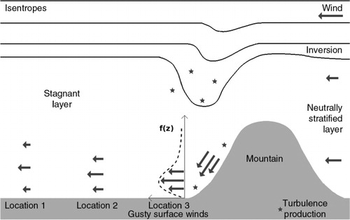
The high-resolution simulations are validated by comparison with the large-scale fields from atmospheric analysis as well as in-situ observations, both from aloft as well as from the surface of the earth. The synoptic-scale fields, as well as many mesoscale features, are in general captured by the control simulation. The most significant errors are found near complex orography, in particular in the main region of interest, in the lee of Mt. Esja in Southwest-Iceland, where the RPAS profiles were made. Here, the control simulation predicts flow which is quite different from what is observed, both aloft and near the surface. Simulations with additional forcing, based on nudging the observed profiles of wind and temperature from the RPAS, reproduce the structure of the local atmospheric flow and compare favourably with surface observations. This is obtained despite the fact that none of the RPAS profiles reaches the inversion aloft; only one profile reaches 1400 m and the others do not reach as high. Overall, the structure of the observed and simulated wind profiles at locations 1–3 (Fig. 4) and the surface observations suggest gravity wave activity above Mt. Esja and a resulting accelerated flow down its lee-side slopes, as is illustrated by the schematic summary in Fig. 12. The strongest winds are observed in a shallow layer at low levels and do not penetrate to the surface most of the time. The wind speed maximum weakens and becomes more diffuse at increasing distances away from the mountain. The flow pattern and the transient nature of the observed winds do indeed indicate active gravity waves and possibly a hydraulic jump. However, prominent gravity waves are not a typical feature of near-to-neutral flow that meets a mountain at only about 7 ms⁻¹. Here, an elevated inversion appears to play a key role. The presence of the inversion and the stable layer at a level of about twice the mountain height correspond nicely to the idealised flows by Vosper (2004) that do indeed show strong waves and downslope acceleration. The present case has a shallow-water Froude number of about 0.5 and H/z_i close to 0.5 where H is the mountain height and z_i is the height of the inversion. This corresponds to the intersection between hydraulic jump-like flows and lee waves in the central part of the flow diagram of Vosper (2004).

Fig. 12 A schematic summary depicting the presumed gravity wave activity aloft and the lee-side accelerated flow, as well as observed wind profiles in lee of the mountain.

No clear dynamic conclusions can be drawn from the nudging of the flow to the profiles observed downstream of Mt. Esja. However, the KEF simulation (nudged with the relocated observed temperature profile from Keflavík) reveals that the sharpness of the inversion is essential for the creation of the strong downslope flow. Temperature modifications of only 1–2 K at the inversion level (Fig. 3) are sufficient to move from a regime of a calm wake (allowing the sea breeze to penetrate) into moderately strong downslope flow. It is not clear why the model does not capture the inversion, but similar errors in the sharpness of small-scale features of the temperature profile are well known to forecasters and they have been associated with limited vertical resolution and excessive mixing/diffusion in the boundary layer scheme (e.g. Teixeira et al., 2008). In connection with the present study and motivated by Gohm et al. (2008) who found strong dependence of the downstream propagation of lee wave rotors and hydraulic jumps on the turbulence parameterization, a number of sensitivity simulations were carried out, with different boundary layer schemes, but they did not reveal any significant improvement. Motivated by series of real-flow simulations from PYREX (Ólafsson and Bougeault, 1997) showing the systematic damping effect of surface friction on mountain waves, some numerical tests were made with reduced surface roughness. These tests gave only slight improvements in the flow (not shown).

Limited resolution of the large-scale atmospheric analysis forcing the model may introduce errors that may be relevant, as noted by Durran and Gingrich (2014) in their study of mesoscale predictability and errors arising from the large scales. The lee-side development may furthermore be strongly affected by non-linear wave dynamics and variability in the impinging flow (Nance and Durran, 1997, 1998), possibly leading to large errors. Studies of ensembles of simulations have in fact shown that downslope windstorms can be highly sensitive to small-scale features in the initial conditions (Reinecke and Durran, 2009). It is however not clear what aspects of the large-scale flow have the greatest impact on the lee-side development or what flow ‘regimes’ are most sensitive, but it may in fact be model dependent (Doyle et al., 2011). This may indeed be true for the sensitivity to the temperature profile revealed in the present study. Finally, wave interference may be relevant when the complex orography on the upstream side of Mt. Esja is taken into account (Grubišić and Stiperski, 2009; Stiperski and Grubišić, 2011).

More systematic three-dimensional observations of boundary layer flow are needed to verify and improve the simulation of boundary layer flows such as those studied here, for example, from additional field experiments with the RPAS. Observations at high-temporal resolution are ideal, and in this context, useful observations of wind, temperatures and turbulent fluxes will be available in the MABLA-experiment (Monitoring the Atmospheric Boundary Layer in the Artic) which is being prepared in the 400 m high mast at Gufuskálar in West-Iceland (Ólafsson et al., 2009). Not only can such observations help improve the simulation of local weather, but also for the momentum fluxes and drag force exerted by the mountain on the flow (e.g. Teixeira et al., 2012). Although the contribution of the current event to the total drag budget is minimal, a deficit may occur if similar events are systematically missed.

It is beyond the current study to analyse the best method to nudge in-situ data, for example, with regard to how well observations from one location in complex terrain may represent the flow at a nearby location, how many profiles to nudge, whether to include observations from the boundary layer, etc. The usefulness of nudging observed profiles of wind and/or temperature into simulations of the atmospheric flow over a mountain is, however, evident in the present case. To what extent this positive result has a general value remains unanswered, but an exploration of the climatology of inversions may be of interest in this connection. Systematic nudging of real-time simulations to atmospheric profiles retrieved by remote sensing may indeed lead to improved forecasting of local weather.

6. Summary and concluding remarks

Unique observations of winds aloft in the lee of Mt. Esja (914 m) in Southwest-Iceland have been analysed together with numerical simulations as well as observations from a dense network of automatic weather stations. The observed profiles of winds and temperature were taken with a small remotely piloted airplane and revealed accelerated flow above the lee-side slopes of the mountain, extending a short distance downstream of the mountain. The observed features have a characteristic scale of a few kilometres and vary in time and space. A sharp temperature inversion observed aloft appears to be very important for the generation of the downslope jet and the associated gravity wave activity. High-resolution atmospheric simulations fail to reproduce the situation, unless details of the temperature profile (the inversion) are reproduced correctly. The successfully simulated lee-side flow exhibits a hydraulic jump-like feature and a structure similar to that observed. The low-level downslope flow can also be reproduced if the atmospheric model is, in addition to large-scale atmospheric analysis, forced with the observed profiles in the lee of the mountain, none of which reach the inversion aloft.

The present study confirms the usefulness of nudging observed profiles to improve simulations of orographic flows. The profiles may be retrieved by remote sensing, conventional radio soundings or by a remotely piloted aircraft, of which the last is least expensive in terms of cost of materials and logistics. The success of the RPAS is not limited to studies of orographic flows; complex sea-breeze situations from the MOSO-project have previously been successfully studied with the RPAS (Jonassen et al., 2012). A system is being developed where in-situ observations from the RPAS may in real-time be ingested into operational and on-demand simulations of weather. Such a system may be used to improve forecasting of local weather in complex and data-sparse terrain, for example, in relation to wind energy applications and during search and rescue operations.

7. Acknowledgements

We thank Joachim Reuder at the University of Bergen for making the SUMO RPAS available during the MOSO-project. This study is a result of a successful and on-going collaboration with Bjarni G. P. Hjarðar at Sorpa waste management and with ISAVIA, the Icelandic Aviation Authority. The work was in part funded by the Icelandic Centre for Research (RANNÍS), through the Icelandic research fund and the Icelandic technology development fund (SARWeather project). We acknowledge three anonymous reviewers for their constructive comments.

References

- Ágústsson H. , Ólafsson H . Simulating a severe windstorm in complex terrain. Meteorol. Z. 2007; 16(1): 111–122.
- Alapaty K. , Seaman N. L. , Devdutta N. S. , Hanna A. F . Assimilating surface data to improve the accuracy of atmospheric boundary layer simulations. J. Appl. Meteorol. 2001; 40: 2068–2082.
- Chen F. , Mitchell K. , Schaake J. , Xue Y. , Pan H. , co-authors . Modeling of land-surface evaporation by four schemes and comparison with FIFE observations. J. Geophys. Res. 1996; 101: 7251–7268.
- Dee D. P. , Uppala S. M. , Simmons A. J. , Berrisford P. , Poli P. , co-authors . The ERA-Interim reanalysis: configuration and performance of the data assimilation system. Q. J. Roy. Meteorol. Soc. 2011; 137(656): 553–597.
- de Rosnay P. , Balsamo G. , Albergel C. , Muñoz-Sabater J. , Isaksen L . Initialisation of land surface variables for numerical weather prediction. Surv. Geophys. 2014; 35(3): 607–621.
- Doyle J. D. , Shapiro M. A. , Jiang Q. , Bartels D. L . Large amplitude mountain wave breaking over Greenland. J. Atmos. Sci. 2005; 62(9): 3106–3126.
- Doyle J. D. , Gaberšek S. , Jiang Q , Bernardet L. , Brown J. M. , co-authors . An intercomparison of T-REX mountain-wave simulations and implications for mesoscale predictability. Mon. Weather Rev. 2011; 139: 2811–2831.
- Dudhia J . Numerical study of convection observed during the winter monsoon experiment using a mesoscale two-dimensional model. J. Atmos. Sci. 1989; 46(20): 3077–3107.
- Durran D. R. , Gingrich M . Atmospheric predictability: why butterflies are not of practical importance. J. Atmos. Sci. 2014; 71(7): 2476–2488.
- Gilliam R. C. , Pleim J. E . Performance assessment of new land surface and planetary boundary layer physics in the WRF-ARW. J. Appl. Meteorol. Climatol. 2010; 49(4): 760–774.
- Gohm A. , Mayr G. J. , Fix A. , Giez A . On the onset of bora and the formation of rotors and jumps near a mountain gap. Q. J. Roy. Meteorol. Soc. 2008; 134(630): 21–46.
- Grubišić V. , Stiperski I . Lee-wave resonances over double bell-shaped obstacle. J. Atmos. Sci. 2009; 66(5): 1205–1228.
- Horvath K. , Koracin D. , Vellore R. , Jiang J. , Belu R . Sub-kilometer dynamical downscaling of near-surface winds in complex terrain using WRF and MM5 mesoscale models. J. Geophys. Res. 2012; 117(D11): 19.
- Hu X.-M. , Klein P. M. , Xue M . Evaluation of the updated YSU planetary boundary layer scheme within WRF for wind resource and air quality assessments. J. Geophys. Res. 2013; 118(18): 10490–10505.
- Janjić Z. I . The step-mountain eta coordinate model: further development of the convection, viscous sublayer, and turbulent closure schemes. Mon. Weather Rev. 1994; 122(5): 927–945.
- Janjić Z. I . Nonsingular implementation of the Mellor-Yamada level 2. 5 scheme in the NCEP meso model. Scientific Report Office Note 437.
- Jonassen M. , Ólafsson H. , Valved A. , Reuder J. , Olseth J . Simulations of the Bergen orographic wind shelter. Tellus A. 2013; 65(19206): 17.
- Jonassen M. O. , Ágústsson H. , Ólafsson H . Impact of surface characteristics on flow over a mesoscale mountain. Q. J. Roy. Meteorol. Soc. 2014; 140(684): 2330–2341.
- Jonassen M. O. , Ólafsson H. , Ágústsson H. , Rögnvaldsson Ó. , Reuder J . Improving high-resolution numerical weather simulations by assimilating data from an unmanned aerial system. Mon. Weather Rev. 2012; 140(11): 3734–3756.
- Langland R. H. , Toth Z. , Gelaro R. , Szunyogh I. , Shapiro M. A. , co-authors . The north pacific experiment (NORPEX-98): targeted observations for improved North American weather forecasts. Bull. Am. Meteorol. Soc. 1999; 80(1): 1363–1384.
- Liu Y. , Bourgeois A. , Warner T. , Swerdin S. , Hacker J . Implementation of observation-nudging based FDDA into WRF for supporting ATEC test operations. Proceeding of Sixth WRF/15th MM5 Users Workshop. Boulder, Colorado, USA: National Center for Atmospheric Research. 1–4.
- Mayer S. , Jonassen M. O. , Sandvik A. , Reuder J . Profiling the Arctic stable boundary layer in Advent valley, Svalbard: measurements and simulations. BoundaryLayer Meteorol. 2012a; 143(3): 507–526.
- Mayer S. , Sandvik A. , Jonassen M. O. , Reuder J . Atmospheric profiling with the UAS SUMO: a new perspective for the evaluation of fine-scale atmospheric models. Meteorol. Atmos. Phys. 2012b; 116(1–2): 15–26.
- Mellor G. L. , Yamada T . Development of a turbulence closure model for geophysical fluid problems. Rev. Geophys. Space Phys. 1982; 20: 851–875.
- Mlawer E. J. , Taubman S. J. , Brown P. D. , Iacono M. J. , Clough S. A . Radiative transfer for inhomogeneous atmospheres: RRTM, a validated correlated-k model for the longwave. J. Geophys. Res. 1997; 102(D14): 16663–16682.
- Nance L. B. , Durran D. R . A modeling study of nonstationary trapped mountain lee waves. Part I: mean flow variability. J. Atmos. Sci. 1997; 54(9): 2275–2291.
- Nance L. B. , Durran D. R . A modeling study of nonstationary trapped mountain lee waves. Part II: nonlinearity. J. Atmos. Sci. 1998; 55(4): 1429–1445.
- Ólafsson H. , Ágústsson H . Gravity wave breaking in easterly flow over Greenland and associated low level barrier- and reverse tip-jets. Meteorol. Atmos. Phys. 2009; 104(3): 191–197.
- Ólafsson H. , Bougeault P . Why was there no wave breaking in PYREX?. Beitr. Phys. Atmos. 1997; 70(2): 167–170.
- Ólafsson H. , Rögnvaldsson Ó. , Reuder J. , Ágústsson H. , Petersen G. N. , Kristjánsson J. E . Monitoring the atmospheric boundary layer in the artic (MABLA): the Gufuskálar project. Proceedings of the 30th International Conference on Alpine Meteorology (ICAM) in Rastatt. 2009; Deutscher Wetterdienst, Annalen der Meteorologie: Germany. 192–193.
- Reinecke P. A. , Durran D. R . Initial condition sensitivities and the predictability of downslope winds. J. Atmos. Sci. 2009; 66(11): 3401–3418.
- Reuder J. , Brisset P. , Jonassen M. O. , Müller M. , Mayer S . The small unmanned meteorological observer SUMO: a new tool for atmospheric boundary layer research. Meteorol. Z. 2009; 18(2): 141–147.
- Reuder J. , Ablinger M. , Ágústsson H. , Brisset P. , Brynjólfsson S. , co-authors . FLOHOF 2007: an overview of the mesoscale meteorological field campaign at Hofsjökull, central Iceland. Meteorol. Atmos. Phys. 2012; 116(1–2): 1–13.
- Rögnvaldsson Ó. , Bao J.-W. , Ólafsson H . Sensitivity simulations of orographic precipitation with MM5 and comparison with observations in Iceland during the Reykjanes Experiment. Meteorol. Z. 2007; 16(1): 87–98.
- Schroeder A. J. , Stauffer D. R. , Seaman N. L. , Deng A. , Gibbs A. M. , co-authors . An automated high-resolution, rapidly relocatable meteorological nowcasting and prediction system. Mon. Weather Rev. 2006; 134: 1237–1265.
- Skamarock W. C. , Klemp J. B. , Dudhia J. , Gill D. O. , Barker D. M. , co-authors . A Description of the Advanced Research WRF version 3.
- Stauffer D. R. , Seaman N. L . Use of four-dimensional data assimilation in a limited-area mesoscale model. Part I: experiments with synoptic-scale data. Mon. Weather Rev. 1990; 118: 1250–1277.
- Stauffer D. R. , Seaman N. L . Multiscale four-dimensional data assimilation. J. Appl. Meteorol. Climatol. 1994; 33: 416–1265.
- Stiperski I. , Grubišić V . Trapped lee wave interference in the presence of surface friction. J. Atmos. Sci. 2011; 68(4): 918–936.
- Teixeira J. , Stevens B. , Bretherton C. S. , Cederwall R. , Klein S. A. , co-authors . Parameterization of the atmospheric boundary layer: a view from just above the inversion. Bull. Am. Meteorol. Soc. 2008; 89(4): 453–458.
- Teixeira M. A. C. , Argain J. L. , Miranda P. M. A . Drag produced by trapped lee waves and propagating mountain waves in a two-layer atmosphere. Q. J. Roy. Meteorol. Soc. 2012; 139B: 964–981.
- Vosper S. B . Inversion effects of mountain lee waves. Q. J. Roy. Meteorol. Soc. 2004; 130: 1723–1748.
- Wyngaard J. C . Toward numerical modeling in the “Terra Incognita.”. J. Atmos. Sci. 2004; 61(7): 1816–1826.