Sampling error of observation impact statistics

Abstract

An observation impact is an estimate of the forecast error reduction by assimilating observations with numerical model forecasts. This study compares the sampling errors of the observation impact statistics (OBIS) of July 2011 and January 2012 using two methods. One method uses the random error under the assumption that the samples are independent, and the other method uses the error with lag correlation under the assumption that the samples are correlated with each other. The OBIS are obtained using the forecast sensitivity to observation (FSO) tool in the Korea Meteorological Administration (KMA) unified model (UM). To verify the self-correlation of the observation impact data, the lag correlations of the observation impact data at 00 UTC in the Northern Hemisphere (NH) summer months (June, July and August 2011) and winter months (December 2011 and January and February 2012) are calculated. The self-correlation approaches zero at 6 days for the summer, whereas it approaches zero at 4 days for the winter, which implies that the observation impact data are serially correlated. The sampling error considering lag correlation is larger than the random error for NH summer and winter. While the random sampling error is approximately 12–13% of the approximation error, the sampling error considering the lag correlation is approximately half of the approximation error of the OBIS. The sampling error that considers the lag correlation of the OBIS is more appropriate for representing the uncertainty in the OBIS because the OBIS at different times are correlated.

• forecast sensitivity to observation
• observation impact statistics
• sampling error

1. Introduction

In recent data assimilation studies, considerable effort has been focused on quantitatively evaluating the effects of observations on numerical weather forecasts. The effects of observations on forecasts have traditionally been assessed using observing system experiments (OSEs). In OSEs, the effects of specific observations are evaluated by comparing the forecast that was integrated from the original analysis made by assimilating the reference set of observations with the forecast integrated from the new analysis made by subtracting (adding) the specific observations from (to) the reference set of observations (e.g. Jung et al., 2010, 2012, 2013). Because of high computational costs, OSEs have been used to estimate the effects of a limited number of observations on specific forecasts. In contrast, the forecast sensitivity to observation (FSO), which is based on the adjoint method, can simultaneously calculate the effects of all of the observations on specific forecasts. Therefore, the FSO is useful for assessing the effect of each observation on forecasts in operational numerical weather prediction (NWP) systems (e.g. Langland and Baker, 2004; Cardinali, 2009; Gelaro and Zhu, 2009; Gelaro et al., 2010; Joo et al., 2013; Jung et al., 2013; Kim and Kim, 2013; Lorenc and Marriott, 2013). The adjoint-based FSO has been used to produce observation impact statistics (OBIS) in operational centres to monitor the effect of each observation on forecasts using a large number of samples (Jung et al., 2013); furthermore, this method has also been used for specific high-impact weather cases in Korea (Kim et al., 2013).

Many statistical methods have been used to evaluate the effects of observations on forecasts in FSO studies. For example, time-averaged observation impacts and the fraction of beneficial observations are calculated using samples extracted from the population. Several FSO studies using global models revealed that the effects of AMSU-A observations (Table 1) on the 24-hour forecast were the largest in operational NWP models, followed by SOUND observations (Cardinali, 2009; Gelaro and Zhu, 2009; Gelaro et al., 2010; Lorenc and Marriott, 2013). In addition, the fraction of beneficial observations that reduced the forecast error among all observations assimilated in several global models was generally 50–55%. In contrast, the fraction of beneficial observations increased by approximately 60% in the regional Weather Research and Forecasting (WRF) model (Jung et al., 2013).

Table 1. Abbreviations for the various observation types used in this study

Abbreviation	Description
METOP-A	First satellite in the operational low earth-orbiting satellite series by the European Organization for the Exploitation of Meteorological Satellites
NOAA	Operational low earth-orbiting satellite series operated by the National Oceanic and Atmospheric Administration of the USA
AMSU-A	Advanced Microwave Sounding Unit-A
MHS	Microwave Humidity Sounder
IASI	Infrared Atmospheric Sounding Interferometer
AIRS	Atmospheric Infrared Sounder
HIRS	High-resolution Infrared Radiation Sounder
GOES	Geostationary Operational Environmental Satellite
MFG	Meteosat First Generation (Meteosat-7) by the European Organization for the Exploitation of Meteorological Satellites
MSG	Meteosat Second Generation (Meteosat-9) by the European Organization for the Exploitation of Meteorological Satellites
MTSAT	Multi-functional Transport Satellite
KMA COMS	Communication, Ocean, and Meteorological Satellite by the Korea Meteorological Administration
SSMI/S	Special Sensor Microwave Imager/Sounder
ASCAT	Advanced Scatterometer
GPSRO	Global Positioning System Radio Occultation
SOUND	Upper-air observations from a radiosonde
DROPSONDE	Upper-air observational device designed to be dropped from an aircraft
PROFL	Upper-air wind profile from a Profiler
PILOT	Upper-air wind profile from a pilot balloon or radiosonde
AIRCRAFT	Upper-air wind and temperature from aircraft
SYNOP	Land surface synoptic weather observations
SHIP	Sea surface weather observation by ship
BUOY	Sea surface weather observation by buoy
TCBOGUS	Tropical cyclone bogus observations generated by national meteorological centres

The uncertainty in the observation impact is subject to various sources such as errors in the verification state, errors in the approximation measure, the sampling error, etc. Lorenc and Marriott (2013) identified three sources of error in the OBIS: observation errors, errors in the verifying analysis and errors in the assumed background error covariances for growing modes. Because it is relatively difficult to quantify the other sources of errors, the uncertainty in the observation impact has been assessed using the sampling error. Therefore, this study is confined to the uncertainty in the observation impact induced by the sampling error. Generally, the random error is used to calculate the sampling error under the assumption that the samples are randomly selected from the population. In fact, the samples of the OBIS are correlated with each other because the same observations and numerical model are used in the assimilation. Nevertheless, the sampling error that considers correlations between the samples has not been used for the OBIS. Therefore, this study proposes a method for determining the realistic sampling error of the OBIS by considering the correlations between the samples. For this purpose, the sampling error that considers correlations between the samples is compared with the sampling error based on random selections for the OBIS in summer and winter months. The OBIS are obtained using the FSO tool (Lorenc and Marriott, 2013; Joo et al., 2013; Kim and Kim, 2013; Kim et al., 2013) of the Korea Meteorological Administration (KMA) unified model (UM). Section 2 introduces the methodology, Section 3 provides the results and Section 4 presents a summary and discussion.

2. Methodology

2.1. Observation impact

The nonlinear forecast error reduction (FER) is defined as follows (Jung et al., 2013; Kim and Kim, 2013):1 where x ^fa and x ^fb are the forecasts integrated from the analysis and background respectively, x ^t is the true state and C is a diagonal norm matrix. Because the true state is not known, the analysis of the 4-dimensional variational data assimilation (4DVAR) system of the KMA UM is used as the true state. The x ^fa –x ^t and x ^fb –x ^t in eq. (1) are replaced by and , respectively. Then, eq. (1) becomes equivalent to2 In Lorenc and Marriott (2013), the right-hand side of eq. (2) is estimated using the full nonlinear model; subsequently, eq. (2) becomes3 where is a change of the forecast state as a result of the assimilation of observations and is the gradient of the FER with respect to δ w _t . δ w _t can be approximated by a formula associated with the observation innovation as in Joo et al. (2013) 4 where δ y, M and K represent the observation innovation, perturbation forecast (PF) model and Kalman gain matrix, respectively. By substituting eq. (4) into eq. (3), the FER in the observation space (i.e. observation impact) can be estimated as5

2.2. Sampling error

The sample (i.e. observation impact) distribution is assumed to be normal if there are sufficient samples. Under the assumption that the OBIS follow a normal distribution, the OBIS can be represented by the average and standard deviation of the sample. The sampling error is the error resulting from the extraction of the sample from the population. The sampling error is usually considered random error because the sample is assumed to be selected randomly from the population. Because the samples used to estimate the observation impact data are not random but correlated by a time lag, the sampling error should be calculated considering the lag correlation between sample data at different times.

2.2.1. The error assuming independent samples.

The random error is defined as the standard deviation divided by the square root of the sample size (Wilks, 2006) as6 where N is the size of the sample, S is the standard deviation of the sample, x _i is the ith sample value and is the sample mean. If the sample distribution is a normal distribution, the standard random error for the 95% (99%) confidence interval is calculated by multiplying the result of eq. (6) by 1.96 (2.58).

2.2.2. The error considering lag correlation.

The observation impact has a time-lagged correlation because the same observations and numerical model are used during the assimilation. To calculate the sampling error for the sample with serial dependence, the time-lagged correlation coefficient of the observation impact must be included in the equation for calculating the sampling error. The error considering the time-lagged correlation is defined as in Wilks (2006),7 where γ ₁ is a lag correlation coefficient when the weak non-stationary time series of the observation impact are lagged by 1 day, and its value ranges from −1 to 1. The error considering the lag correlation in eq. (7) is calculated considering the lag correlation coefficient, different from the random error in eq. (6). If the data have positive lag correlations, then the sampling error increases, as shown in Wilks (2010).

3. Results

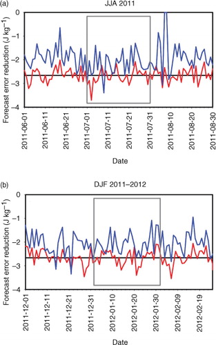
Figure 1 shows the time series of the nonlinear and approximated FER that correspond to 00 UTC in the Northern Hemisphere (NH) summer months (June, July and August 2011) and winter months (December 2011 and January and February 2012). The nonlinear FER oscillates around the average of −2.658774 J kg⁻¹ for summer and −2.662570 J kg⁻¹ for winter, which implies that the data assimilation effect fluctuates daily, as reported in Jung et al. (2013) and Kim and Kim (2013). The approximated FER generally underestimates the nonlinear FER. The difference between the nonlinear FER and approximated FER is the approximation error. The magnitude of the approximation errors oscillates around the average of 0.6903 J kg⁻¹ for summer and 0.5981 J kg⁻¹ for winter. The random sampling errors oscillate around the average of 0.0861 J kg⁻¹ for summer and 0.0805 J kg⁻¹ for winter, which correspond to 12.4% in summer and 13.4% in winter of the approximation errors. The approximation error is caused by the approximated formulation of FER [e.g. eq. (5)], simplified moist physics in the PF and adjoint models, and dry energy norm used to define the FER (Langland and Baker, 2004; Gelaro et al., 2007; Jung et al., 2013), and/or observation errors, errors in the verifying analysis, and errors in the assumed background error covariances for growing modes (Lorenc and Marriott, 2013). In addition, nothing is known about how the overall error in approximation will be distributed among individual observation impact estimates for various observation types, although this is another source of uncertainty in OBIS. The magnitude of the sampling error may be changed when considering the time-lagged correlation between the FER. The random error and error considering the lag correlation are calculated and analysed for July 2011 and January 2012 (grey boxes in Fig. 1). The 31 individual sample distributions for July 2011 and January 2012 are similar to the normal distribution (not shown), and the sample standard deviations are ±0.4998 J kg⁻¹ for July 2011 and ±0.5217 J kg⁻¹ for January 2012.

Fig. 1 Time series (red line) and average (black line) of the nonlinear forecast error reduction (FER) and time series (blue line) of the approximated FER at 00 UTC analysis time in the Northern Hemisphere (NH) for (a) June, July and August 2011 and for (b) December 2011 and January and February 2012. The period for calculating the sampling error is denoted by the grey box.

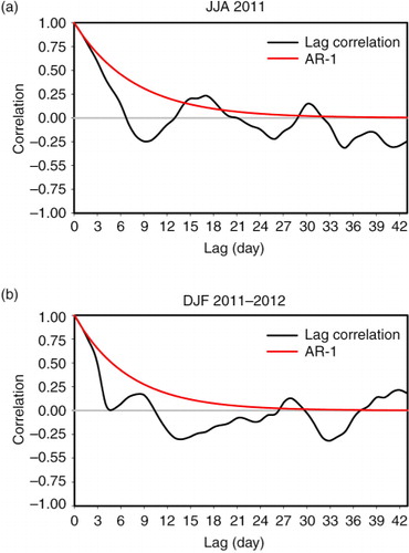
Figure 2 shows the time-lagged correlation coefficient (γ) of the 5-day moving average of the observation impacts of the NH summer and winter months. Because non-stationary time-series data have a serial dependency (Wilks, 2006), the sampling error of the non-stationary time-series data deviates from the realistic sampling error calculated from the stationary time-series data without the serial dependency. The lag correlation γ is calculated using a 5-day moving average of the observation impact to decrease the serial dependency of the time series. The 5-day moving average is calculated by averaging the observation impact for the five previous days, beginning with the present day. Hereafter, lag-k represents the lag correlation between the moving-average time series with a 0-day lag and the moving-average time series with a k-day lag. Therefore, the value of lag-0 is one because of the perfect self-correlation of the time series data. The lag correlation in the NH summer months starts from one and decreases to zero at a 6-day lag (Fig. 2a), which implies that the time series at lag-0 is not correlated with the time series at lag-6. Subsequently, the lag correlation oscillates and converges to zero until lag-30. The self-correlation for the NH winter months disappears if both time series are lagged by 4 days (Fig. 2b). Subsequently, the lag correlation irregularly oscillates, and the time lag for the winter is shorter than that for the summer because of the strong baroclinicity in the NH midlatitude in the winter, as reported by Langland and Baker (2004). Therefore, due to the correlated time series of the OBIS, the sampling error needs to be calculated considering the lag correlation between samples. This study also examines whether the first-order auto regression (AR-1) model can realistically approximate the lag correlation (γ ₁). The k-th autocorrelation ρ _k in the AR-1 model is defined as ρ _{k =} (γ ₁) ^k (Wilks, 2006). The AR-1 autocorrelation is similar to the lag-1, lag-2 and lag-3 correlations for the NH summer and winter months (Figs. 2a and b), which implies that the AR-1 autocorrelation can be used rather than the actual lag correlation for 1 to 3 days of time lag and that the AR-1 autocorrelation can be used to calculate the error considering the time-lagged correlation in eq. (7).

Fig. 2 The lag correlation (black line) calculated from the 5-day moving average of the observation impact in the NH for (a) June, July and August 2011 and for (b) December 2011 and January and February 2012. The lag correlation using the AR-1 model is represented by the red line.

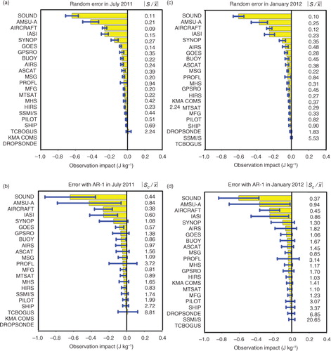
Figure 3 shows the time-averaged observation impact, random error and sampling error using the AR-1 autocorrelation for July 2011 and January 2012. For both months, the observation impact of SOUND is the greatest, followed by those of AMSU-A, AIRCRAFT, IASI and SYNOP. Because the OBIS are obtained at every 00 UTC during the study period, the observation impact of SOUND is the greatest. In contrast, the observation impact of the satellite data was the greatest in previous studies (e.g. Langland and Baker, 2004; Cardinali, 2009; Gelaro and Zhu, 2009; Gelaro et al., 2010; Joo et al., 2013; Jung et al., 2013; Lorenc and Marriott, 2013) because these previous studies were based on the observation impact data collected at 00, 06, 12 and 18 UTC. The sampling errors that consider the lag correlation in Figs. 3b and d have larger error bars compared to the random sampling error in Figs. 3a and c in both summer and winter. The lag correlation was based on the 1-day lag (i.e. AR-1 autocorrelation) in both July 2011 and January 2012. To examine the reliability of the statistical estimates, the relative standard deviation (coefficient of variation) of the sample assuming independent samples () and the error considering lag correlation () are shown as numbers next to the bars in Fig. 3. The relative standard error is the absolute value of the ratio between the sample standard deviation and the sample mean. The time-averaged OBIS with the lower relative standard error have a more precise estimation. For the random error, the relative standard errors of all observation types are smaller than 1, except for TCBOGUS in July 2011 and SSMI/S and DROPSONDE in January 2012. The time-averaged observation impact of TCBOGUS in July 2011 was positive, which indicates that assimilating TCBOGUS produces a greater forecast error than the forecast without its assimilation. The effect of SSMI/S in January 2012 is very small and close to zero. For the error considering lag correlation, the relative standard errors of all observation types increase approximately 3.9 times for summer and 3.7 times for winter, compared with the random error. For the four observation types which show the larger observation impact (i.e. SOUND, AMSU-A, AIRCRAFT and IASI), the relative standard errors are less than 1, which implies that the time-averaged OBIS are relatively precise for these observation types compared with other observation types. As the observation impact decreases, the relative standard errors oscillate showing increasing trend.

Fig. 3 The time-averaged observation impact (yellow bar, J kg⁻¹) and sampling error (blue line, J kg⁻¹) using (a, c) the random error and (b, d) the error using the AR-1 autocorrelation, stratified with the observation type for July 2011 and for January 2012, respectively.

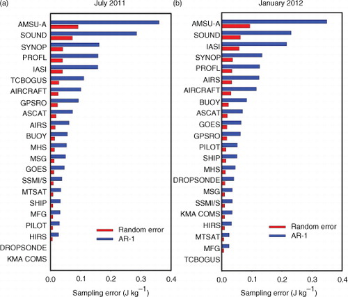
Figure 4 shows the random error, the error considering the lag correlation (i.e. AR-1) in July 2011 and January 2012. Compared to the random error in July 2011 and January 2012, the error considering the lag correlation increases for all of the observations (Fig. 4). Because the sampling error considering lag correlation is much larger than the random sampling error, a percentage of the sampling error in the total error (Fig. 1) increases. The sampling errors considering lag correlation oscillate around the average of 0.3381 J kg⁻¹ for summer and 0.3003 J kg⁻¹ for winter, which correspond to 48.9% in summer and 50.2% in winter of the approximation errors. Therefore, the magnitude of the sampling error considering lag correlation is approximately half of the approximation error, which is a considerable amount of the total uncertainties associated with the observation impact estimation.

Fig. 4 The sampling error (bar, J kg⁻¹) stratified with the observation type for (a) July 2011 and (b) January 2012. The random error (red) and the error using the AR-1 autocorrelation (blue).

4. Summary and discussion

The sampling errors of the OBIS of July 2011 and January 2012 are calculated using two methods and then compared. The first method uses the random error under the assumption that the samples are independent. The second method uses the error that considers the lag correlation under the assumption that the samples at different times are correlated because the OBIS are calculated using the same numerical model and observations. The lag correlation is calculated using a 5-day moving average of the observation impact at 00 UTC in the NH summer months (June, July and August 2011) and winter months (December 2011 and January and February 2012). The 5-day moving average decreases the serial dependence of the sample time series. The serial dependence of the moving-averaged time series disappears if the time series is lagged by 6 days for the NH summer months and by 4 days for the NH winter months. The time lag without the serial dependence for winter is shorter than that for summer because of the strong baroclinicity in the NH midlatitude in the NH winter (Langland and Baker, 2004). Because the time series of the OBIS are correlated, the realistic sampling error should be calculated considering the lag correlation between samples. In addition, the AR-1 autocorrelation is similar to the lag correlation for 1 to 3 days of lag for both months, which implies that the AR-1 autocorrelation can be used instead of the lag correlation to calculate the sampling error.

The error that considers the lag correlation (i.e. 1-day lag correlation in the NH summer and NH winter; AR-1 autocorrelation) is larger than the random error for all of the observations for both NH summer and winter. As a result, the relative standard errors of the observation impact of all the observation types increase for the sampling error considering lag correlation compared to the random sampling error.

Because the OBIS are estimated under several assumption, the approximation error (i.e. the difference between the nonlinear and approximated FER by the observation impact) could be caused by many factors: the approximated formulation, simplified moist physics in the PF and adjoint models, and dry energy norm (Langland and Baker, 2004; Gelaro et al., 2007; Jung et al., 2013), observation errors, errors in the verifying analysis, and errors in the assumed background error covariances for growing modes (Lorenc and Marriott, 2013), and the sampling error. Compared to the random sampling error which corresponds to 12–13% of the approximation error, the sampling error considering lag correlation corresponds to approximately half of the approximation error, which implies that a considerable portion of the total uncertainties associated with the observation impact estimation may be due to the sampling error.

Therefore, it is concluded that the realistic sampling error that considers the lag correlation between the samples of the OBIS is larger than the random error and that the sampling error considering the lag correlation is more appropriate than the random error for representing the uncertainty in the OBIS because the OBIS are correlated. The magnitude of the sampling error when considering lag correlation of the OBIS is approximately a half of the approximation error, which implies that a considerable portion of the uncertainty in the OBIS could be explained by the sampling error when considering lag correlation. The future work would be quantifying other sources of the approximation error in the OBIS. Other sources of the errors [e.g. errors in the verifying analysis, and errors in the assumed background error covariances for growing modes mentioned in Lorenc and Marriott (2013)] would be spatially correlated. The error that incorporates spatial correlation of the OBIS would further help understanding characteristics of the uncertainties associated with the OBIS.

5. Acknowledgements

The authors thank two anonymous reviewers for their valuable comments. The authors thank the Numerical Weather Prediction Division of the Korea Meteorological Administration and the UK Met Office for providing computer facility support and resources for this study. The Korea Meteorological Administration Research and Development Program under Grant CATER 2012-2030 supported this study.

References

- Cardinali C . Monitoring the observation impact on the short-range forecast. Q. J. Roy. Meteorol. Soc. 2009; 135: 239–250.
- Gelaro R. , Langland R. H. , Pellerin S. , Todling R . The THORPEX observation impact intercomparison experiment. Mon. Weather Rev. 2010; 138: 4009–4025.
- Gelaro R. , Zhu Y . Examination of observation impacts derived from observing system experiments (OSEs) and adjoint models. Tellus A. 2009; 61: 179–193.
- Gelaro R. , Zhu Y. , Errico R. M . Examination of various-order adjoint-based approximations of observation impact. Meteorol. Z. 2007; 16(6): 685–692.
- Joo S. , Eyre J. , Marriott R . The impact of Metop and other satellite data within the Met Office global NWP system using an adjoint-based sensitivity method. Mon. Weather Rev. 2013; 141: 3331–3342.
- Jung B.-J. , Kim H. M. , Auligne T. , Zhang X. , Huang X.-Y . Adjoint-derived observation impact using WRF in the western North Pacific. Mon. Weather Rev. 2013; 141: 4080–4097.
- Jung B.-J. , Kim H. M. , Kim Y.-H. , Jeon E.-H. , Kim K.-H . Observation system experiments for Typhoon Jangmi (200815) observed during T-PARC. Asia-Pacific J. Atmos. Sci. 2010; 46: 305–316.
- Jung B.-J. , Kim H. M. , Zhang F. , Wu C.-C . Effect of targeted dropsonde observations and best track data on the track forecasts of Typhoon Sinlaku (2008) using an Ensemble Kalman Filter. Tellus A. 2012; 64: 14984. http://dx.doi.org/10.3402/tellusa.v64i0.14984 .
- Kim S. , Kim H. M. , Kim E.-J. , Shin H.-C . Forecast sensitivity to observations for high-impact weather events in the Korean Peninsula. Atmosphere. 2013; 21(2): 163–172. (in Korean with English abstract).
- Kim S. M. , Kim H. M . Observation impact estimation using a forecast sensitivity to observation (FSO) method in the global and East Asia regions. EGU General Assembly 2013. 2013. Vienna, Austria, 7–12 April 2013.
- Langland R. H. , Baker N. L . Estimation of observation impact using the NRL atmospheric variational data assimilation adjoint system. Tellus A. 2004; 56: 189–201.
- Lorenc A. C. , Marriott R . Forecast sensitivity to observations in the Met Office Global numerical weather prediction system. Q. J. Roy. Meteorol. Soc. 2013; 140: 209–224.
- Wilks D. S . Statistical Methods in the Atmospheric Sciences.
- Wilks D. S . Sampling distributions of the Brier score and Brier skill score under serial dependence. Q. J. Roy. Meteorol. Soc. 2010; 136: 2109–2118.