Development and evaluation of a new regional coupled atmosphere–ocean model in the North Sea and Baltic Sea

Abstract

A new regional coupled model system for the North Sea and the Baltic Sea is developed, which is composed of the regional setup of ocean model NEMO, the Rossby Centre regional climate model RCA4, the sea ice model LIM3 and the river routing model CaMa-Flood. The performance of this coupled model system is assessed using a simulation forced with ERA-Interim reanalysis data at the lateral boundaries during the period 1979–2010. Compared to observations, this coupled model system can realistically simulate the present climate. Since the active coupling area covers the North Sea and Baltic Sea only, the impact of the ocean on the atmosphere over Europe is small. However, we found some local, statistically significant impacts on surface parameters like 2 m air temperature and sea surface temperature (SST). A precipitation-SST correlation analysis indicates that both coupled and uncoupled models can reproduce the air–sea relationship reasonably well. However, the coupled simulation gives slightly better correlations even when all seasons are taken into account. The seasonal correlation analysis shows that the air–sea interaction has a strong seasonal dependence. Strongest discrepancies between the coupled and the uncoupled simulations occur during summer. Due to lack of air–sea interaction, in the Baltic Sea in the uncoupled atmosphere-standalone run the correlation between precipitation and SST is too small compared to observations, whereas the coupled run is more realistic. Further, the correlation analysis between heat flux components and SST tendency suggests that the coupled model has a stronger correlation. Our analyses show that this coupled model system is stable and suitable for different climate change studies.

• coupled atmosphere–ocean model
• regional climate
• North Sea and Baltic Sea
• air–sea interaction
• correlation analysis
• SST tendency

1. Introduction

In recent years, uncertainties in climate model projections have become of great interest because a wide range of future projections have become available comprising a combination of various emission scenarios and different climate models. Coupled atmosphere–ocean general circulation models are usually used for such climate change studies. The concept of ocean–atmosphere coupling has become essential for explaining processes on time scales ranging from seasonal to decadal variability (Fedorov, 2008). The coupling mechanism is straightforward: sea surface temperature (SST) anomalies induce diabatic heating or cooling of the atmosphere and alter the atmospheric circulation and consequently wind stresses and heat fluxes at the ocean surface (Fedorov, 2008). Hence, the components of the climate system should not be treated separately. Due to the coarse resolution of global models, detailed local features, particularly along complex coastlines, cannot be resolved. Hence, for climate change impact and adaptation studies as well as for climate-process studies of regional importance high-resolution regional coupled models are essential.

As a major tool for regional climate change studies, different regional coupled models have been developed during the past two decades and used to study the climate over Europe. During the earlier stage, the ocean model component was relatively simple and flux corrections are necessary to avoid artificial drifting of the coupled system away from realistic sea state conditions. Gustafsson et al. (1998) have coupled the regional weather forecasting model HIRLAM with a horizontally averaged basin model for the Baltic Sea. The ocean model is provided with surface pressure, 2 m temperature, 2 m humidity, total cloudiness and 10 m wind to calculate energy fluxes for coupling, rather than using the fluxes computed by the atmospheric model. Hagedorn et al. (2000) developed a fully coupled high-resolution regional climate model based on REMO and the Kiel Baltic Sea model. This atmosphere–ocean model was coupled directly via corresponding fluxes without flux corrections and gave realistic results for autumn 1995. However, the coupling to an ice model was still missing. Döscher et al. (2002) developed a coupled atmosphere–ice–ocean model with interactive, consistent flux coupling for the Baltic Sea. This coupled system was free of drift and suitable for long-term climate studies (Döscher et al., 2002; Räisänen et al., 2004; Kjellström et al., 2005).

These previously discussed regional coupled models focused on the Baltic Sea, a semi-enclosed brackish sea. However, the water and salt exchanges between the North Sea and the Baltic Sea play an important role for the physical and bio-chemical processes in the Baltic Sea. The effective saltwater intrusions into the Baltic Sea are controlled by special atmospheric conditions causing substantial sea level differences between Kattegat and the western Baltic Sea (Schinke and Matthäus, 1998; Schimanke et al., 2014). Therefore, it is vital to include both the Baltic Sea and North Sea within a coupled model system. Lehmann et al. (2004) simulated the major inflow event in March 2003 with a coupled model called BALTIMOS and showed that this exceptional inflow event was realistically simulated. Schrum et al. (2003) carried out hindcast experiments with a regional coupled atmosphere/ice/ocean model for the whole North Sea and Baltic Sea. Their model was stable over a full seasonal cycle and on the regional scale the coupling turned out to be a clear improvement compared to an uncoupled atmosphere–standalone model run. Tian et al. (2013) used a two-way nested fine-grid to resolve the Danish straits and argued that the atmosphere in the Baltic land–sea transition was more sensitive to high-resolution modelled SST fields. Their coupled and uncoupled simulations only showed minor differences over land in the Baltic coastal region. In addition, Mikolajewicz et al. (2005) and Döscher et al. (2010) studied the Arctic climate with regional coupled models including also the North Sea and the Baltic Sea in their domains. However, the resolutions of their models were coarse and not sufficient to capture the detailed climate in the North Sea and Baltic Sea regions.

In summary, previous studies either focused only on the Baltic Sea region or the integration period was limited, the model resolution was too coarse or essential model component like sea ice or river runoff were lacking. The aim of this study is to extend the current scope and to provide an effective tool for climate change studies in Europe, which takes regional ocean–atmosphere interaction from the North Sea and Baltic Sea into account.

In Section 2, the model components, coupling procedure and experimental design are described. In Section 3, the results from a hindcast simulation are evaluated compared to different observational datasets. Thereafter, the impact of air–sea coupling on the relationships between atmospheric variables and SST are further analysed. In the last section, the model results are summarised and discussed.

2. Model descriptions and experimental design

2.1. Rossby Centre regional climate model RCA4

The atmospheric component of our coupled model is the regional model RCA4. Originally RCA4 is based on the numerical weather prediction (NWP) model HIRLAM (Undén et al., 2002) and is a primitive equation hydrostatic model using a terrain-following hybrid vertical coordinate. Technically, the RCA4 model is the climate version of the operational model HIRLAM. Since 1997, the Rossby Centre at Swedish Meteorological and Hydrological Institute (SMHI) has released four versions of RCA: RCA1 (Rummukainen et al., 2001), RCA2 (Jones et al., 2004), RCA3 (Samuelsson et al., 2011) and RCA4 (Kupiainen et al., 2014) used in our coupled model system.

Compared to the previous version (RCA3), several parameterisations have been improved or new ones have been implemented. A new lake model (Flake) is utilised in RCA4. Flake is a freshwater lake model capable of predicting the vertical temperature structure and mixing conditions in lakes of various depths on time scales from a few hours to many years (Mironov, 2008). This scheme has been used in various NWP models, climate modelling, and other numerical prediction systems for environmental applications (Martynov et al., 2010; Mironov et al., 2010). The Kain and Fritsch (1993) convection scheme has been updated to the Bechtold Kain-Fritsch scheme (Bechtold et al., 2001) which separates the shallow and deep convection processes. A convection closure based on convective available potential energy (CAPE) (Bechtold et al., 2001) is applied in RCA4 which may be more suitable for simulations with high resolution. The soil hydrology in RCA4 is divided into a forest and an open land tile. The inclusion of soil carbon in RCA4 has reduced the overestimated soil–air heat transfer observed in RCA3 and improved the simulated diurnal temperature range, particularly in the northern part of the model domain. This can be explained by improved soil temperature simulation because the top organic soil has higher hydraulic conductivity, lower thermal conductivity and higher porosity compared to mineral soils. Another important improvement treats the effect of snow albedo. Pirazzini (2009) found that the positive snow albedo-temperature feedback is an important factor in the high-latitude amplification of the global warming. The modifications in prognostic snow albedo have reduced a warm bias in cold climate conditions. The usage of global ECOCLIMAP land-use and soil conditions allows this model to transfer easily to different domains. RCA4 has been used for different domains in the Coordinated Regional Climate Downscaling Experiment (CORDEX) project, including Europe, South-Asia, Arctic and Africa. For other physical parametrisations and a more detailed description, we refer to Samuelsson et al. (2011).

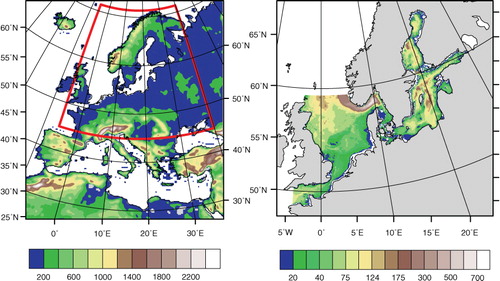
In this study, RCA4 has been set up for the European domain at a 0.22 degree spherical, rotated latitude/longitude grid with 40 vertical levels (Fig. 1). The model domain covers all of the European continental area, the Mediterranean Sea and a broad area of the North Atlantic Ocean.

Fig. 1 RCA4 domain and topography (the red square is the domain of the river routing model CaMa-Flood) (left) and the ocean model domain and bathymetry (right) (unit: meter).

2.2. Regional setup of ocean model NEMO and sea ice model LIM3

The oceanic part of the coupled model is based on the Nucleus for European Modelling of the Ocean (NEMO) model, which is a primitive equation model (Madec, 2011). This model solves the incompressible and hydrostatic primitive equations using a free surface. In the vertical, a surface following z-coordinate with partial steps is utilised to allow for an enhanced resolution of the vertical levels near the sea surface. Within the NEMO framework, the sea ice model LIM3 is coupled to the ocean component. LIM3 includes the representation of both the thermodynamic and dynamic processes. A comprehensive description of the sea ice model is given in Vancoppenolle et al. (2009).

The model domain covers the whole Baltic Sea, the English Channel and the North Sea with open boundaries along the western entrance of the English Channel and along the northern boundary of the North Sea between the Orkney Islands and Norway (Fig. 1). This setup ensures that the entrance to the Baltic Sea is far away from the open boundary and provides a sufficiently large buffer for wind forcing in the North Sea. Along the open boundary the astronomical tides from the Oregon State University Tidal Inversion Model with 11 tidal harmonics are prescribed. Climatological monthly mean salinity and temperature from Levitus data (Antonov et al., 1998; Boyer et al., 1998) are used as a lateral boundary for the simulations. A simple radiation scheme is used for baroclinic velocities at the open boundary. Horizontal and vertical resolutions amount to 2 nautical miles (about 3.7 km) and 56 vertical levels. For a detailed physical description of the configuration the reader is referred to Dieterich et al. (2013) and Hordoir et al. (2013).

The ocean model was spun up for 20 years using surface forcing fields derived from a RCA4 dynamically downscaled simulation driven by ECMWF's 40-year reanalysis (ERA40) data (Uppala et al., 2005). Restart files have been saved to perform the hindcast runs analysed in this paper.

2.3. River routing model

The river routing component of our coupled model is a Catchment-based Macro-scale Floodplain model (CaMa-Flood) (Yamazaki et al., 2011). CaMa-Flood is designed as a continental-scale distributed model. The prominent feature of this model is that the global river network is discretised to hydrological unit-catchment to allow for efficient computation at the global scale and for easy coupling into model systems (Yamazaki et al., 2011). In comparison with other routing models, the CaMa-Flood model has several distinctive advantages. In addition to river discharge, the flood stage (water level and flood area) is also explicitly represented, which enables possible direct comparisons between simulated flood stage and satellite observations besides traditional validation with gauge data (Yamazaki et al., 2012). The implemented local inertial equation and adaptive time step scheme make the simulation computationally efficient (Yamazaki et al., 2013). This model has been setup for the North Sea and Baltic Sea catchment areas (Fig. 1).

2.4. Coupling and experimental strategy

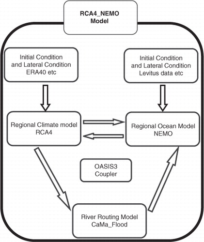
Within the coupled system, the atmospheric component model RCA4, the oceanic component NEMO (sea ice model LIM3 is included) and the runoff model CaMa-Flood are run as three separate executables. To build up this coupled modelling system, the Ocean Atmosphere Sea Ice Soil Simulation Software (OASIS3) coupler (Valcke, 2013) integrates the sub-models simultaneously (Fig. 2). The coupler works in a sequential fashion with synchronous coupling of the different model components with joint physical interfaces at different time intervals. This two-way coupled system passes heat fluxes, freshwater fluxes, momentum fluxes, non-solar heat flux derivative and sea level pressure from the atmosphere to the ocean, and the atmosphere receives SST, sea ice concentration, sea ice surface temperature and sea ice albedo from the NEMO model for the interactively coupled area. The atmosphere–ocean coupling frequency is set to 3 hours. To provide river runoff for NEMO, coastal river runoff from CaMa-Flood is sent to NEMO at daily frequency.

Fig. 2 Schematic diagram of the coupled model system (The sea ice model LIM3 is part of NEMO and not coupled via OASIS3).

The hindcast simulation is performed for the period 1979 to 2010. In order to investigate the effect of coupling, the different model components are also run in standalone mode. The RCA4 standalone run is directly driven by ERA-Interim data (Dee et al., 2011) and NEMO is driven with forcing fields from RCA4-standalone downscaled ERA-Interim simulation for the same period.

2.5. Validation data

To evaluate our model, various observational datasets are used. Atmospheric parameters which include 2 m temperature, precipitation and total cloud cover are compared with Climate Research Unit (CRU) TS3.21 data (Harris et al., 2014). Due to the different resolution between RCA4 and CRU data, the CRU data are interpolated to the RCA4 grid with the bicubic interpolation method and the CRU 2 m temperature is corrected with vertical lapse rate to eliminate the effect of orography. SST data between 1982 and 2010 are taken from the National Oceanic and Atmospheric Administration (NOAA) optimum interpolation 0.25 degree daily SST analysis dataset (OISST). This dataset is generated from several data sources including SST data from Advanced Very High Resolution Radiometer (AVHRR), Advanced Microwave Scanning Radiometer (AMSR) and in situ data from ships and buoys. As precipitation from the CRU dataset is only available on land points, 0.5 degree global precipitation data from Deutscher Wetterdienst (DWD) are used. This dataset is combined with the Hamburg Ocean Atmosphere Parameters and Fluxes from Satellite (HOAPS) Data are derived from EUMETSAT Satellite Application Facility on Climate Monitoring (CMSAF) and the Global Precipitation Climatology Centre (GPCC) data from 1987 to 2008. OISST and DWD precipitation data are interpolated to a 25 km grid covering the North Sea and Baltic Sea.

3. Model evaluation

3.1. Atmospheric variables

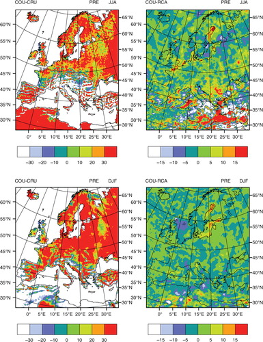
The quality of future projections of climate change depends on the ability of the RCMs to reproduce the present-day climate. In particular, the effect of coupling has to be evaluated for the present-day climate. Considering the limitation due to missing observations, only the last 30-year (1981–2010) simulation results are analysed. Figure 3 illustrates the mean seasonal differences of 2 m temperature (1981–2010) between the coupled and the uncoupled atmosphere run and observations for summer and winter.

Fig. 3 Seasonal mean 2 m temperature (T2M) differences between the coupled run and observations (COU-CRU), and between the coupled run and the uncoupled atmosphere run (COU-RCA) for summer (JJA, top panel) and winter (DJF, bottom panel) (unit: K). Hatching indicates differences with significance level exceeding 95%.

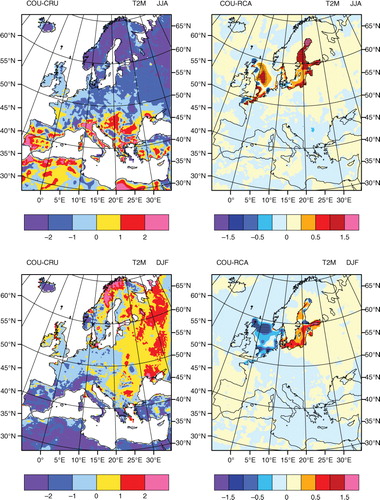
In the coupled simulation RCA4 is slightly warmer during summer around the North Sea and the Baltic Sea (max 0.25 K over land away from the coast and max 1.5 K over the Baltic) compared to the standalone RCA4 run (Fig. 3). The Mediterranean coastal region is somewhat cooler in the coupled simulation but the changes are not significant and do not exceed 0.25 K in summer. Both changes reduce the bias of the uncoupled atmosphere-standalone simulation indicating that air–sea coupling improves the 2 m temperature slightly. However, the largest impact on the temperature can be found over the coupled ocean areas. Here, the coupling leads to an increased 2 m temperature over the Baltic Sea and North Sea during summer, particularly in the northern Baltic Sea. A significance test shows that most of the differences over the coupled region exceed the 95% significance level.

In winter, the 2 m temperature is warmer over the Baltic Sea, but colder over the North Sea in the coupled case compared to the uncoupled atmosphere run. During winter the bias over land compared to observations is smaller than during summer. Winter biases in northern Europe are found to be around 1 K, while summer biases in the same area are around 2 K. The difference can be explained, at least partly, by the snow albedo–temperature feedback mechanism active in winter. In the Baltic Sea, the ice–albedo feedback reinforces differences between coupled and uncoupled simulations. Actually, in the coupled run, sea ice cover is underestimated compared to observations (see below) resulting in earlier ice melt, lower sea surface albedo and increased absorption of solar radiation. Hence, in early summer SSTs are higher in the coupled simulation compared to the uncoupled run, which is forced with SSTs from ERA-Interim. A significance test shows that only the area with differences larger than 1 K (i.e. parts of the coupled Baltic Sea and North Sea areas) exceeds the 95% significance level.

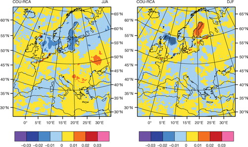
The 2 m temperature is strongly affected by other atmospheric parameters, e.g. total cloud cover. The altered total cloud cover has the potential to change the surface heat balance and alter the temperature distribution. Compared to the uncoupled atmosphere run, in the coupled run summertime reduced cloud cover (Fig. 4) is connected to warmer 2 m temperature over the Baltic and North seas. This suggests a warming influence of short wave radiation. In wintertime, the impact of cloud cover on short wave radiation is minor. The increased cloud cover over the Baltic Sea (Fig. 4) is connected to warmer air temperature. The underestimated sea ice cover has a positive contribution to long wave radiation absorption in the Baltic Sea. This indicates a warming influence of long wave radiation by increased cloud cover. Decreased cloud cover over the North Sea is connected to colder air temperature by decreased long wave radiation absorption.

Fig. 4 Seasonal mean differences of total cloud cover between the coupled run and the uncoupled atmosphere run (COU-RCA) for summer (JJA, left) and winter (DJF, right) (unit: fraction). Hatching indicates differences with significance level exceeding 95%.

Figure 5 shows the mean seasonal differences for precipitation. The precipitation is overestimated by about 20–30% over European continental areas in all seasons. The spatial distribution of the difference between the coupled and uncoupled case shows that there is no unique spatial pattern for summer and winter (Fig. 5). However, there is still a different deviation distribution between the North Sea and Baltic Sea. In winter we find a wet deviation in the Baltic Sea and dry deviation in the North Sea, which is consistent with the 2-m air–temperature distribution (Fig. 3), i.e. a warm deviation over the Baltic Sea and a cold deviation over the North Sea. However, the significance test shows that only some of the deviations exceed the 95% significance level. These are mainly located over the northern Baltic Sea.

Fig. 5 Seasonal mean precipitation (PRE) relative differences (%) between the coupled run and observations (COU-CRU), and between the coupled run and the uncoupled atmosphere run (COU-RCA) for summer (JJA, top panel) and winter (DJF, bottom panel). Hatching indicates differences with significance level exceeding 95%.

In the coupled system, sea ice concentration is updated from NEMO every 3 hours. Our analysis suggests that the sea ice cover is usually underestimated. Due to feedback mechanisms the reduced sea ice cover leads to a warmer air temperature and more cloud cover. This could partly cause more precipitation over the Baltic Sea in winter. In summer, the clouds from the coupled simulation are reduced over the North Sea and the Baltic Sea (Fig. 4). This is also reflected by heat flux changes (see below). Over the Baltic Sea, the net short wave radiation maximum difference shows that in summer the coupled ocean receives about 6 W/m² more than the standalone ocean run, but loses in winter about 2 W/m² more than in the uncoupled ocean simulation (not shown). The change of solar shortwave radiation at the water surface is caused mainly by the higher cloudiness calculated from the coupled model. The total cloud cover regulates the amount of sunlight reaching the surface and has altered the long wave and short wave radiation reaching the surface. The increased short wave radiation in the atmospheric model could lead to warmer SSTs and increase the oceanic heat loss due to latent heat flux (LatH). This tends to provide more water vapour to the atmosphere and has an impact on the atmospheric baroclinicity and thus has the principle potential to modulate the large-scale atmospheric circulation pattern.

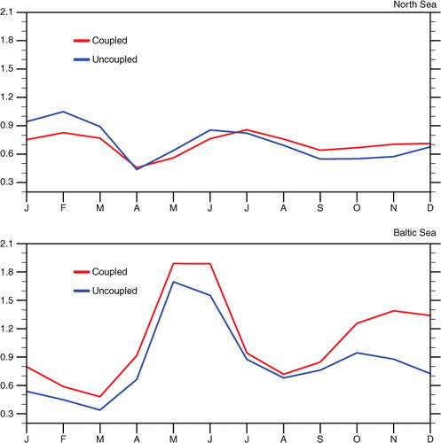
To distinguish between the different behaviour over the Baltic Sea and North Sea, the spatially averaged differences between coupled run and uncoupled atmosphere run for 2 m temperature, precipitation (Fig. 6) and heat fluxes components (Fig. 7) are calculated. In the Baltic Sea the coupled simulation produces higher 2 m temperature with more precipitation on annual average (Fig. 6). The general agreement of seasonal variation in 2 m temperature and precipitation is high except for April–June. During those months, the temperature difference between coupled and uncoupled run are largest, but the precipitation is almost unchanged. In the North Sea, the 2 m temperature and precipitation are in agreement throughout the year. The coupled simulation shows significantly colder 2 m temperature between December and April, in accord with reduced precipitation.

Fig. 6 2 m temperature (top, unit: K) and precipitation (bottom, unit:%) differences between the coupled run and the uncoupled atmosphere run in the North Sea and Baltic Sea.

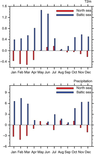
Fig. 7 Heat flux differences between the coupled run and the uncoupled atmosphere run in the North Sea (top) and Baltic Sea (bottom) (unit: W/m²). Positive values indicate fluxes into the ocean.

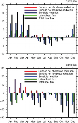
Figure 7 shows the monthly mean differences between the coupled run and uncoupled atmosphere run for heat flux components and total heat fluxes in the North Sea and Baltic Sea. In the Baltic Sea, the total heat flux differences are negative in all the months except March. This implies that the atmosphere receives more energy from the ocean and also can partly explain why 2 m temperature has increased. The dominant contributors for heat flux differences are the sensible and LatHs. From March to March, the net long wave radiation also makes a substantial contribution. In the North Sea, we find contrasting differences between the warm and cold seasons. There is a large increase in the total heat fluxes from December to April and slight decrease between June and October. Similar to the Baltic Sea, the sensible and LatHs are also the major contributors to the differences of surface energy balances.

3.2. Sea surface temperature

The above analysis of atmospheric fields indicates that the coupling exhibits distinct influence especially over the active coupling region in the North Sea and Baltic Sea. Differences in SST have direct or indirect effects on the spatial distribution of atmospheric parameters. In this section, we assess the impact of atmospheric forcing and coupling on the ocean model. The seasonal mean SST in the North Sea and Baltic Sea are compared with high-quality satellite data. In the coupled simulation, the SST in the North Sea is slightly underestimated in the cold seasons and overestimated in the warmer seasons (not shown). The difference between the coupled run and observations do usually not exceed 1 K in most parts of the region (not shown). In contrast, the SST in the Baltic Sea has positive differences during the whole year and the biases are also slightly higher compared to the North Sea. However, the bias exceeds 1.5 K only very rarely and is spatially restricted (not shown). In general, the SST and the 2 m temperature over the ocean are closely related. Consequently, the 2 m temperature biases discussed in the previous section can be explained to a large degree by the bias of SST.

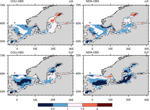
To investigate the modelled SST towards satellite SST, the Root Mean Square Error (RMSE) is calculated for different seasons for both the coupled and the uncoupled ocean-standalone simulation (Fig. 8). In the North Sea, both simulations have similar quality, except that the uncoupled simulation has a slightly larger RMSE along the southern coast of Norway during winter. This difference could be related to a different freshwater exchange between the North Sea and the Baltic Sea through the Danish straights. In the Baltic Sea, the coupled simulation has somewhat larger errors during both seasons with exception of the northern Baltic Sea during winter. This spatial error distribution is related to differences in the modelled and prescribed sea ice extent. Moreover, it should be noted that SST observations from satellites suffer from imperfect ice detection, which might also contribute to the computed RMSE.

Fig. 8 RMSE of SST between the coupled model and observations (COU-OBS, left) and between the uncoupled ocean model and observations (NEM-OBS, right) for summer (JJA, top panel) and winter (DJF, bottom panel) (unit: K).

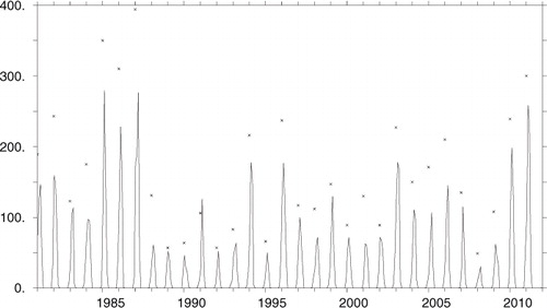
Figure 9 shows the sea ice extent from the coupled simulation (monthly mean) and observations (annual maximum). Currently, we can only access monthly mean sea ice extents from the ocean model, which is not directly comparable with the observed annual maximum based on daily values. However, the variability seems to be captured reasonably well. For instance, winters with a large sea ice extent in the model correlated with observed high maximum sea ice extent and vice versa. To gain better insights into the quality of simulated two-dimensional sea ice cover, the mean ice concentration averaged between 1981 and 2010 is visually compared with the climatological ice atlas (Udin et al., 1982) (not shown). The climatological mean ice concentrations from both simulations are underestimated. Moreover, the sea ice cover in the coupled simulation is slightly smaller compared to the uncoupled ocean model run, but the main features of the Baltic Sea ice cover are well represented. The reduced sea ice cover leads to a positive contribution to the warmer SST in the Baltic Sea.

Fig. 9 Monthly mean Baltic Sea ice extent from the coupled simulation (black line) and observed maximum ice extent (black crosses) (unit: 10⁹ m²).

Overall, the climatological seasonal mean analysis shows that, compared to observations and the uncoupled ocean run, the SST in the coupled simulation is slightly overestimated in the North Sea and the Baltic Sea. Only the winter SST is slightly improved in the North Sea. Figure 10 shows the seasonal cycle of SST RMSE in the North Sea and the Baltic Sea. The seasonal cycle is generally in good agreement between the coupled and the uncoupled ocean simulations, and both have similar maxima and minima. However, the RMSE shows a strong seasonal difference between the North Sea and Baltic Sea. In the North Sea, the coupled run has a smaller RMSE in the first half-year and the difference between the coupled run and uncoupled ocean run is generally small, between 0.1 and 0.2 K. In the Baltic Sea, both simulations show strong seasonal variations in the RMSE with highest values in May and June. In general, the uncoupled ocean run performs slightly better. However, the differences between the coupled run and uncoupled ocean run are rather small. Only during November and December differences in the RMSE reach values close to 0.5 K.

Fig. 10 Spatial averaged RMSE of SST for the coupled run and uncoupled atmosphere run in the North Sea (top panel) and Baltic Sea (bottom panel) (unit: K).

4. Correlation analysis of local air–sea interaction

From the above evaluation, the coupling of atmospheric and oceanic components has a clear effect on both the SST and atmospheric variables. But it is not clear whether the coupled model has produced a valid air–sea relationship. The lead–lag correlation analysis between the atmospheric variables and SST is widely used to study the nature of local air–sea interaction (von Storch, 2000; Wu et al., 2006). To further reveal the forcing–response relationship between atmospheric variables and SST, the correlation between atmospheric variables and SST tendency are also calculated (Cayan, 1992; Wu et al., 2006). In the following, the SST tendency in a specific month is the difference between the SST of the next month minus the SST of the previous month divided by two (Wu et al., 2006). Hence, the analysis is based on monthly data.

4.1. Correlation between precipitation and SST

Firstly, we analyse the correlation between precipitation and SST. The precipitation as an important atmospheric parameter has a strong impact on the freshwater flux into the North Sea and particularly into the Baltic Sea. Due to the shallow mixed layer, there is a quick response between the atmosphere and the Baltic Sea. To check whether the coupled model can reproduce the relationship between precipitation and SST, Fig. 11 depicts the correlation of precipitation-SST and precipitation-SST tendency for observations, uncoupled atmosphere run and coupled run. Before calculating the correlation, the observed and ERA-Interim SSTs and the observed precipitation are interpolated to the RCA4 grid with a horizontal resolution of 25 km. The correlations are calculated for the period 1988 to 2008, which is the same period as covered by observed precipitation. As seen in Fig. 11, the correlations between precipitation and SST from observations are positive in most of the Baltic Sea and negative in most of the North Sea. Positive correlations indicate an impact of the ocean on the atmosphere. In this case, the atmosphere has a positive response to SST fluctuations. The correlation is weak in the centre of the Baltic Sea. Compared to the Baltic Sea, the North Sea has a deeper bathymetry and an open boundary towards the North Atlantic Ocean. This difference may cause the contrast in air–sea relationship between these two regions. In observations the correlations between precipitation and SST tendency in the North Sea and Baltic Sea are negative, with particularly high negative correlations in the North Sea. This indicates the dominant role of the atmosphere for SST changes (Wu et al., 2006). In the Baltic Sea, we found a large negative precipitation-SST tendency correlation in the centre of the basin.

Fig. 11 Top panel: correlation between precipitation and SST (left) and correlation between precipitation and SST tendency (right) for observations (OBS). Middle panel: as top panel except for uncoupled atmosphere run (UCOU). Bottom panel: as top panel except for the coupled run (COU).

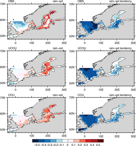
Now, we compare the correlation of precipitation and SST from the coupled run with both observations and the uncoupled atmosphere run. The results of the uncoupled and the coupled runs show similar patterns of correlation between precipitation and SST. However, there are significant differences in the location and magnitude compared to observations. In the Baltic Sea, the general feature is well reproduced, although both models cannot capture the weak correlation in the centre of the basin. In the North Sea, the magnitude of correlation is underestimated in both model runs. The negative correlations in the northern part of the North Sea are much weaker. In the centre of the Baltic Sea, the correlation of precipitation and SST tendency is in the coupled run slightly better simulated than in the uncoupled atmosphere run. As the uncoupled atmosphere run is forced with prescribed SSTs taken from ERA-Interim data, precipitation has no causal influence on the SST tendency. Therefore, the discrepancies between the coupled run and uncoupled atmosphere run are due to the impact of air–sea coupling.

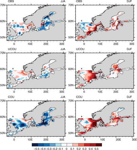
From the analysis of SSTs, we already found a strong seasonal variability. To further study seasonal features of the air–sea interaction, Fig. 12 shows the precipitation-SST correlation in summer and winter for the observations, the uncoupled atmosphere run and the coupled run. In winter, the spatial distribution of the correlation is similar to the annual correlation. A positive correlation is seen over most of the Baltic Sea region. The coupled run has slightly higher correlation coefficients which indicate that the air–sea coupling enhances the effect of SST on the atmosphere. In the North Sea the negative correlation coefficients are underestimated in the uncoupled atmosphere run, and slightly improved in the coupled run. The most pronounced effects of air–sea coupling are found in summer. The spatial correlation patterns in the Baltic Sea in summer are in contrast to the annual patterns (Fig. 11). High negative correlation reveals that the forcing of the atmosphere on the ocean is strong and this feature is well captured by the coupled model. The uncoupled atmosphere run has a too weak correlation, particularly in the northern Baltic Sea. In the North Sea, the coupled run has a much higher negative correlation compared to the observation and the uncoupled run. This indicates that the effect of atmospheric forcing on the ocean is stronger in the North Sea and the response of SST to atmospheric forcing is overestimated. The uncoupled atmosphere run cannot capture this feature due to the lacking air–sea interaction.

Fig. 12 Top panel: precipitation-SST correlation for observation (OBS) in summer (JJA, left column) and winter (DJF, right column). Middle panel: as top panel except for the uncoupled atmosphere simulation (UCOU). Bottom panel: as the top panel except for the coupled simulation (COU).

4.2. Correlations between heat flux components and SST

In this section, we analyse the correlations between heat fluxes and SST. Due to the lack of high-resolution and high-quality heat flux data, the following analysis focuses only on differences between the coupled and the uncoupled atmosphere runs due to the impact of air–sea coupling. Figures 13 and 14 show the correlation coefficients in summer and winter between sensible heat flux (SenH), latent heat flux (LatH), surface net short wave radiation (swr), surface net long wave radiation (lwr) and SST for the uncoupled atmosphere run and the coupled run, respectively. The relationships between the heat flux components and SST show pronounced seasonal differences (Figs. 13 and 14). All correlation coefficients differ largely in spatial distribution between summer and winter. In summer, sensible heat flux, latent heat flux and long wave radiation show negative correlations with SST. Only the correlations between short wave radiation and SST are positive. The relationships between heat flux components and SST tendency are different. In summer, sensible heat flux, latent heat flux and short wave radiation have positive correlations, whereas long wave radiation has negative correlations (not shown). In winter, short wave radiation and latent heat flux have negative correlation coefficients or weak positive correlations, whereas sensible heat flux and long wave radiation have a positive correlation or a weak negative correlation in a small part of the region (not shown). This suggests that sensible heat flux and long wave radiation are strongly affected by SST changes, whereas short wave radiation and latent heat flux are mainly regulated by atmospheric variations. However, the positive correlations between all four flux components and SST tendency suggest that these four heat flux components contribute to SST variations, particularly sensible and latent heat fluxes (not shown).

Fig. 13 Correlations between sensible heat flux (SenH), latent heat flux (LatH), short wave radiation (swr), long wave radiation (lwr) and SST (from top to bottom) in Summer (JJA, left column) and winter (DJF, right column) for the uncoupled atmosphere run.

Fig. 14 Similar to Fig. 13 except for the coupled run.

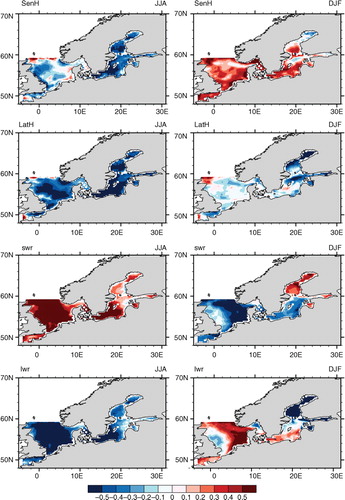
Now, we compare the correlation coefficient patterns between the coupled (Fig. 14) and the uncoupled atmosphere runs (Fig. 13). Both models produce similar relationships between heat flux components and SST. The main difference caused by air–sea coupling is the magnitude of correlation, especially for the correlation between heat fluxes and SST tendency (not shown). Due to the feedback on SST in the coupled run, the correlation between heat flux components and SST tendency is much larger in the Baltic Sea in summer. We also find spatial differences, particularly in the northern Baltic Sea during winter. This is mainly due to differently simulated sea ice concentrations. In the uncoupled atmosphere run, the heat fluxes have no influences on the SST tendency. Hence, positive correlations between heat flux components and SST tendency in the coupled run are higher which explains the warmer SSTs in the Baltic Sea.

4.3. Lead–lag correlations between heat flux components and SST

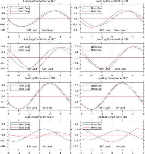
To further understand the differences of forcing–response relationship in the North Sea and the Baltic Sea between the coupled run and the uncoupled atmosphere run, the temporal evolution of lead–lag correlation is calculated for the area mean values. Figure 15 shows the lead–lag correlations between sensible heat flux (SenH), latent heat flux (LatH), short wave radiation (swr), long wave radiation (lwr) and SST for the North Sea and Baltic Sea from the coupled run and the uncoupled atmosphere run. The evolution of lead–lag correlation from the coupled simulation resembles the uncoupled atmosphere simulation with some fluctuations. The heat flux components show negative correlations when SST leads and positive correlations when SST lags. Except for the short wave radiation, there are pronounced differences between the coupled run and the uncoupled atmosphere run. The positive correlation between sensible heat flux and SST in the Baltic Sea for the coupled run at lag 0 and when the SST is leading indicates that the air–sea coupling has a positive feedback between SST forcing and the atmosphere. In the North Sea, the negative correlation between latent heat flux and SST is also higher in the coupled run (Fig. 15). Another significant difference between the coupled and the uncoupled atmosphere run is the correlation between long wave radiation and SST in the Baltic Sea. The coupled run has larger correlation when SST leads or lags. As SST has a more direct effect on the long wave radiation, the correlation in the uncoupled atmosphere run is much smaller due to the lack of feedback with prescribed SST.

Fig. 15 Lead/lag correlations between sensible heat flux (SenH), latent heat flux (LatH), short wave radiation (swr), long wave radiation (lwr) and SST (from top to bottom) for the uncoupled atmosphere run (left column) and the coupled run (right column) (X-axis: month).

5. Discussion and summary

In this study, we describe the coupled regional climate model RCA4-NEMO, which includes an ocean model, a sea ice model, an atmospheric model and a river routing model. The atmosphere domain covers all Europe, while a full ocean–atmosphere coupling is active for the North Sea and the Baltic Sea region. The atmosphere and the ocean are closely connected through fluxes of heat, moisture and momentum at the sea surface. To study the impact of air–sea coupling in more detail, three experiments are performed between 1979 and 2010; two standalone runs with RCA4 and NEMO, respectively, and one coupled run. The results from 1981 to 2010 are analysed. Here we describe the basic physical performance of the coupled model and investigate the interaction between the atmosphere and the ocean.

The atmospheric 2 m temperature shows biases varying with seasons. Away from the actual coupled area, differences between coupled and uncoupled atmosphere simulations are small. SST differences of up to 1.5 K are found with higher values in the Baltic Sea compared to the North Sea. Differences between the Baltic Sea or the North Sea averaged SSTs of the coupled and the uncoupled case are small, with the uncoupled ocean simulation performing slightly better in the Baltic Sea. Precipitation is overestimated by about 20–30% over European continental areas in all seasons, and only small differences are seen between coupled and uncoupled simulation. Both the coupled and the uncoupled simulations underestimate the sea ice cover.

The evaluation shows that pronounced atmospheric differences between the coupled and the uncoupled atmosphere case usually occur in the North Sea and the Baltic Sea region, as judged from effects on atmospheric surface temperature, cloudiness and precipitation. We find that the coupled atmosphere is slightly warmer around the Baltic Sea compared to the standalone atmosphere run year-round. The North Sea area is slightly warmer during summer and slightly colder during winter. The coupled simulation tends to give more total cloud cover over most of the domain in winter. The total heat flux from the atmosphere to the ocean is affected by the coupling in different ways for the Baltic Sea and the North Sea. At the coupled Baltic Sea surface, the atmosphere receives more heat from the ocean as in the uncoupled atmosphere run. Over the North Sea, the coupling effect depends on the season. During summer, the atmosphere receives more heat from the ocean, while the opposite is seen during winter. Both 2 m temperature and precipitation over the Baltic Sea and North Sea are systematically affected by the coupling. Compared to the uncoupled atmosphere simulation, both 2 m temperature and precipitation are increased for the Baltic Sea and decreased or neutral for the North Sea.

To further analyse the nature of local air–sea interaction, correlation analysis is used for SST and precipitation, whereby both variables serve as a general indicator of the state and response of the ocean and the atmosphere. Compared to observations, the coupled simulation gives slightly more realistic correlations. A negative precipitation-SST tendency correlation is seen in the North Sea and the Baltic Sea, which indicates that the coupled model can reproduce the atmospheric contribution of SST changes. A seasonal correlation analysis shows an air–sea interaction with strong seasonal dependence. Strongest discrepancies between coupled and uncoupled atmosphere simulations occur during summer.

The correlations of heat flux components and SST also show strong seasonality. All correlations show a contrast in spatial distribution between summer and winter. In summer, the positive correlation coefficient with the SST tendency indicates that the heat flux components have positive contributions to SST changes except the long wave radiation. In winter, sensible heat flux and long wave radiation are strongly affected by SST changes, and short wave radiation and latent heat flux are mainly regulated by atmospheric variation. But the positive correlations with SST tendency for all four flux components suggest these four heat flux components contribute to SST fluctuations, particularly sensible heat flux and latent heat flux. The coupled and the uncoupled atmosphere runs have similar spatial distribution with slight differences in magnitude.

A coupled regional model adds process descriptions as well as complexity to standalone models. Therefore, improved physical performance of all components is not self-evident, because increased complexity increases the degree of freedom of the overall system. On that background, a performance in the same class as the standalone runs is a success in a first order consideration. In addition, we can identify selected improvements and specific effects due to the coupled setup. The long integration period indicates that this model system is stable and suitable for different climate change studies. Here we analyse performance and behaviour of physical fields and their interconnection dependent on the way of coupling to other model components on a monthly basis.

Many other issues remain undiscussed, e.g. the coupling effects on a daily time scale and a more general consideration of added value of coupling for atmospheric and oceanic climate scenarios. Next steps could also consider the impact of coupling on extreme events. The atmosphere responds more quickly to a varying SST and this could impact on the synoptic scale phenomena, which possibly directly affect the extreme events. We are also aiming at an evaluation of the river routing model.

6. Acknowledgements

Part of the work has been funded by Swedish Mistra-SWECIA programme funded by Mistra (the Foundation for Strategic Environmental Research). The authors would like to thank Dr. Dai Yamazaki providing the river routing model CaMa-Flood. ECMWF, CRU, DWD, CMSAF and NOAA are acknowledged for the use of their data. The work by CD, AH, RH, HEMM and SS has been financed by the Swedish Research Council for Environment, Agricultural Sciences and Spatial Planning (FORMAS) within the project ‘‘Impact of changing climate on circulation and biogeochemical cycles of the integrated North Sea and Baltic Sea system’’ (grant no. 214-2010-1575) and by the German Federal Ministry of Transport, Building and Urban Development (BMVBS) within the program “Impacts of Climate Change on Waterways and Navigation” (KLIWAS). The research presented in this study is part of the Baltic Earth programme (Earth System Science for the Baltic Sea region, see http://www.baltic-earth.eu). The authors would like to thank two anonymous reviewers for their helpful comments.

References

- Antonov J. I. , Levitus S. , Boyer T. P. , Conkright M. E. , O'Brien T. D. , co-authors . World Ocean Atlas 1998 Vol. 1: Temperature of the Atlantic Ocean. 1998; Washington, DC: US Government Printing Office. NOAA Atlas NESDIS 27.
- Bechtold P. , Bazile E. , Guichard F. , Mascart P. , Richard E . A mass-flux convection scheme for regional and global models. Q. J. Roy. Meteorol. Soc. 2001; 127: 869–886.
- Boyer T. P. , Levitus S. , Antonov J. I. , Conkright M. E. , O'Brien T. , co-authors . World Ocean Atlas 1998 Vol. 4: Salinity of the Atlantic Ocean. 1998; Washington, DC: US Government Printing Office. NOAA Atlas NESDIS 30.
- Cayan D. R . Latent and sensible heat flux anomalies over the northern oceans: driving the sea surface temperature. J. Phys. Oceanogr. 1992; 22: 859–881.
- Dee D. , Uppsala S. , Simmons A. , Berrisford P. , Poli P. , co-authors . The ERA-interim reanalysis: configuration and performance of the data assimilation system. Q. J. Roy. Meteorol. Soc. 2011; 137(656): 553–597.
- Dieterich C. , Schimanke S. , Wang S. , Väli G. , Liu Y. , co-authors . Evaluation of the SMHI Coupled Atmosphere–Ice–Ocean Model RCA4-NEMO. 2013; 1–80. SMHI Report Oceanography No.47, SMHI, Norrköping.
- Döscher R. , Willén U. , Jones C. , Rutgersson A. , Meier H. E. M. , co-authors . The development of the regional coupled ocean–atmosphere model RCAO. Boreal Environ. Res. 2002; 7: 183–192.
- Döscher R. , Wyser K. , Meier H. M. M. , Qian M. , Redler R . Quantifying Arctic contributions to climate predictability in a regional coupled ocean–ice–atmosphere model. Clim. Dyn. 2010; 34: 1157–1176.
- Fedorov A. V . Cuff D. , Goudie A . Ocean–atmosphere coupling. Oxford Companion to Global Change. 2008; Oxford University Press, Oxford. 369–374.
- Gustafsson N. , Nyberg L. , Omstedt A . Coupling of a high-resolution atmospheric model and an ocean model for the Baltic Sea. Mon. Weather Rev. 1998; 126: 2822–2846.
- Hagedorn R. , Lehmann A. , Jackob D . A coupled high resolution atmosphere–ocean model for the BALTEX Region. Meteorol. Z. 2000; 9: 7–20.
- Harris I. , Jones P. D. , Osborn T. J. , Lister D. H . Updated high-resolution grids of monthly climatic observations – the CRU TS3.10 dataset. Int. J. Climatol. 2014; 34: 623–642.
- Hordoir R. , Dieterich C. , Basu C. , Dietze H. , Meier H. E. M . Freshwater outflow of the Baltic Sea and transport in the Norwegian current: a statistical correlation analysis based on a numerical experiment. Continent. Shelf Res. 2013; 64: 1–9.
- Jones C. , Willen U. , Ullerstig A. , Hansson U . The Rossby Centre regional atmospheric climate model part I: model climatology and performance for the present climate over Europe. Ambio. 2004; 33(4–5): 199–210.
- Kain J. S. , Fritsch J. M . Emanuel K. A. , Raymon D. J . Convective parameterisations for mesocale models: the Kain-Fritsch scheme. The Representation of Cumulus Convection in Numerical Models. 1993; Boston, MA: American Meteorological Society. 1–246.
- Kjellström E. , Döscher R. , Meier H. E. M . Atmospheric response to different sea surface temperatures in the Baltic Sea: coupled versus uncoupled regional climate model experiments. Nord. Hydrol. 2005; 36(4–5): 397–409.
- Kupiainen M. , Jansson C. , Samuelsson P. , Jones C. , Willén U. , co-authors . Rossby Centre regional atmospheric model, RCA4, Rossby Center News Letter. 2014. Online at: http://www.smhi.se/en/Research/Research-departments/climate-research-rossby-centre2-552/1.16562 .
- Lehmann A. , Lorenz P. , Jacob D . Modelling the exceptional Baltic Sea inflow events in 2002–2003. Geophys. Res. Lett. 2004; 31 L21308.
- Madec G . NEMO Ocean Engine. 2011; Paris, France: IPSL. User Manual 3.3.
- Martynov A. , Sushama L. , Laprise R . Simulation of temperate freezing lakes by one-dimensional lake models: performance assessment for interactive coupling with regional climate models. Boreal Environ. Res. 2010; 15: 143–164.
- Mikolajewicz U. , Sein D. V. , Jacob D. , Königk T. , Podzun R. , co-authors . Simulating Arctic sea ice variability with a coupled regional atmosphere–ocean–sea ice model. Meteorol. Z. 2005; 14: 793–800.
- Mironov D. , Heise E. , Kourzeneva E. , Ritter B. , Schneider N. , co-authors . Implementation of the lake parameterisation scheme FLake into the numerical weather prediction model COSMO. Boreal Environ. Res. 2010; 15: 218–230.
- Mironov D. V . Parameterization of Lakes in Numerical Weather Prediction. Description of a Lake Model. 2008; Offenbach am Main, Germany: Deutscher Wetterdienst. 1–41. COSMO Technical Report, No. 11.
- Pirazzini R . Challenges in snow and ice albedo parameterizations. Geophysica. 2009; 45(1–2): 41–62.
- Räisänen J. , Hansson U. , Ullerstig A. , Döscher R. , Graham L. P. , co-authors . European climate in the late 21st century: regional simulations with two driving global models and two forcing scenarios. Clim. Dyn. 2004; 22: 13–31.
- Rummukainen M. , Räisänen J. , Bringfelt B. , Ullerstig A. , Omstedt A. , co-authors . A regional climate model for northern Europe: model description and results from the downscaling of two GCM control simulations. Clim. Dyn. 2001; 17(5–6): 339–359.
- Samuelsson P. , Jones C. , Willen U. , Ullerstig A. , Gollvik S. , co-authors . The Rossby Centre Regional Climate model RCAS3: model description and performance. Tellus A. 2011; 63: 4–23.
- Schimanke S. , Dieterich C. , Meier H. E. M . An algorithm based on sea-level pressure fluctuations to identify major Baltic inflow events. Tellus A. 2014; 66: 23452. http://dx.doi.org/10.3402/tellusa.v66.23452 .
- Schinke H. , Matthäus W . On the causes of major Baltic inflows an analysis of long time series. Continent. Shelf Res. 1998; 18: 67–97.
- Schrum C. , Huebner U. , Jacob D. , Podzum R . A coupled atmosphere/ice/ocean model for the North Sea and the Baltic Sea. Clim. Dyn. 2003; 21: 131–151.
- Tian T. , Boberg F. , Christensen O. , Christensen J. , She J. , co-authors . Resolved complex coastlines and land–sea contrasts in a high-resolution regional climate model: a comparative study using prescribed and modelled SSTs. Tellus A. 2013; 65: 19951. http://dx.doi.org/10.3402/tellusa.v65i0.1995 .
- Udin I. , Sahlberg J. , Leppäranta M . Climatological Ice Atlas for the Baltic Sea, Kattegat, Skagerrak and Lake Vänern (1963–1979). 1982; Norrköping, Sweden: SMHI. Technical Report 04–11.
- Undén P. , Rontu L. , Järvinen H. , Lynch P. , Calvo J. , co-authors . HIRLAM-5 Scientific Documents. 2002; Norrköping, Sweden: SMHI. 1–144. HIRLAM Report.
- Uppala S. M. , Kållberg P. W. , Simmons A. J. , Andrae U. , Da Costa Bechtold V. , co-authors . The ERA-40 re-analysis. Q. J. Roy. Meteorol. Soc. 2005; 131: 2961–3012.
- Valcke S . The OASIS3 coupler: a European climate modelling community software. Geosci. Model Dev. 2013; 6: 373–388.
- Vancoppenolle M. , Fichefet T. , Goosse H. , Bouillon S. , Madec G. , co-authors . Simulating the mass balance and salinity of arctic and Antarctic sea ice. Ocean Model. 2009; 27: 33–53.
- von Storch J. S . Signature of air–sea interactions in a coupled atmosphere–ocean GCM. J. Clim. 2000; 13: 3361–3379.
- Wu R. , Kirtman B. P. , Pegion K . Local air–sea relationship in observation and model simulations. J. Clim. 2006; 19: 4914–4932.
- Yamazaki D. , Kanae S. , Kim H. , Oki T . A physically-based description of floodplain inundation dynamics in a global river routing model. Water Resour. Res. 2011; 47 W04501.
- Yamazaki D. , de Almeida G. A. M. , Bates P. D . Improving computational efficiency in global river models by implementing the local inertial flow equation and a vector-based river network map. Water Resour. Res. 2013; 49: 7221–7235.
- Yamazaki D. , Lee H. , Alsdorf D. E. , Dutra E. , Kim H. , Kanae S. , Oki T . Analysis of the water level dynamics simulated by a global river model: A case study in the Amazon River. Water Resour. Res. 2012; 48 W09508.