On downscaling probabilities for heavy 24-hour precipitation events at seasonal-to-decadal scales

Abstract

We examine a method for predicting variations in the probabilities and occurrence of intense local 24-hour precipitation events over seasonal, annual, and 5-yr intervals. The wet-day mean μ can be used to describe the exponential distribution for the wet-day amounts, and provides a basis for forecasting the likelihood of seeing an event above a given threshold. A regression-based downscaling model is calibrated on annual μ and wet-day frequency f _w , respectively, and then tested on seasonal to multi-annual scales. The probabilities for heavy precipitation statistics are taken as the product between a fitted cumulative exponential distribution for the wet-day amounts μ and f _w . The annual number of heavy precipitation events is estimated from the annual probability, where a 90% confidence interval on the number is computed using the 5 and 95 percentiles of a binomial distribution for the predicted probability. The analysis identifies a strong link between large-scale predictors such as mean sea-level pressure or surface temperature and the wet-day frequency. There was a weaker dependency of the wet-day mean to large-scale predictors, which suggests that local-scale processes have a stronger influence on the 24-hour precipitation amounts. The results also suggest that similar physical processes influence the wet-day mean μ on different timescales except for during winter, and that similar physical processes may explain the wet-day frequency on seasonal to annual time scales. The implication is that models calibrated on annual data samples in some cases can give skilful predictions on seasonal time scales.

• Precipitation
• wet-day mean
• wet-day frequency
• seasonal-to-decadal forecast
• validation
• statistical downscaling

To access the supplementary material to this article, please see Supplementary files under ‘Article Tools’.

1. Introduction

Can we make skilful forecasts of precipitation statistics seasons to decades ahead, given large-scale patterns in surface temperature and mean sea level pressure (SLP)? Local climate information is important for the users in addition to their credibility, salience, and legitimacy. Barsugli et al. (2013) proposed that establishing the credibility of downscaled climate data is more than just evaluation against historical observations. Skilful forecast on lead times from seasons to decades would provide a valuable basis for decision making for many sectors in our society (Palmer et al., 2000). For instance, such forecasts could guide farmers on choices regarding when and what to sow (Doblas-Reyes et al., 2007), hydroelectric power producers on how much water to retain in the reservoirs, and manufacturers on the volume of production. Furthermore, early warnings on extreme precipitation can help mitigating flooding and provide valuable time for making necessary preparations. One question is whether such early warning systems are possible, even if we could predict the general state and flow of the oceans and the air masses. Here we try to answer this question in more specific terms: whether it is possible to predict local 24-hour precipitation statistics for a season, year, or a decade, given a representative description of the regional large-scale conditions. We also test the hypothesis whether dependencies between large-scale conditions and local rainfall found on annual timescales are valid for seasonal or decadal timescales.

1.1. Background

Several studies in the past have investigated the possibility of skilful seasonal forecasts for large-scale regional conditions based on general circulation models (GCMs) and statistical forecasting models (Barnett and Preisendorfer, 1987; Barnston et al., 1994; Palmer and Anderson, 1994; Dix and Hunt, 1995; Johansson et al., 1998; Stockdale et al., 1998; Derome et al., 2001, 2005; Rodwell and Doblas-Reyes, 2006). Some studies have suggested that a blend of results from different types of GCMs may improve the forecast skill (Krishnamurti et al., 1999; Yun et al., 2003); however, the question whether such blending results in a real enhancement of skill has also been questioned (Weigel et al., 2008).

Seasonal forecasting has been far more challenging for the North Atlantic and European region than for the Tropics, where the El Niño Southern Oscillation (ENSO) is a major factor. There have been some studies on teleconnections between ENSO and Europe (Lloyd-Huges and Saunders, 2002), but so far with little success in enhancing seasonal forecasting model skill. A major effort was undertaken to develop a European multimodel ensemble system for seasonal to inter-annual prediction, DEMETER (Palmer et al., 2004) and ENSEMBLES (Linden and Mitchell, 2009). A large part of the seasonal variability over Europe can be linked to variations in the North Atlantic Oscillation (NAO), the jet stream, and planetary Rossby waves; hence, skilful seasonal forecasts need to forecast their future state (Derome et al., 2005; Johansson, 2007). Other factors that may have an effect on the subsequent season over Europe may include the snow cover or the Arctic sea ice (Ueda et al., 2003; Benestad et al., 2010; Orsolini et al., 2011). However, it is difficult to find a systematic effect for some of these conditions. Furthermore, their effect may vary with season. It is also possible that the stratosphere may play a role for seasonal variations (Baldwin and Dunkerton, 2001; Thompson et al., 2002; Baldwin et al., 2003; Brönnimann et al., 2004; Cagnazzo and Manzini, 2009).

The seasonal forecasting capability has improved over time (Kharin and Zwiers, 2003; Palmer, 2004; George and Sutton, 2006; Stocker et al., 2013), especially in the Tropics. Some of the improvement can be attributed to more advanced models, but part of the progress can also be linked to better model initialisation (Zhang and Frederiksen, 2003; Li et al., 2008) or a better understanding of phenomena such as teleconnections (Hawkins et al., 2002). Recent seasonal forecasting activity has also included prognoses for storm statistics (Compo and Sardeshmukh, 2004; Vitard et al., 2007).

Murphy et al. (2010) reviewed the state on predicting decadal climate variability and change. They provided an overview of phenomena with decadal time scales, such as the NAO, the Atlantic Multi-decadal Oscillation (AMO), the Tropical Atlantic surface air temperature Gradient Oscillation (TAG), the North Pacific Oscillation (NPO), the Pacific Decadal Oscillation (PDO), and the Inter-decadal Pacific Oscillation (IPO). The state-of-the-art models are able to simulate key features of the most prominent of these modes, they argued, and at least on a global scale, simulated decadal temperature variability has been shown to be realistic. They also noted that precipitation variance in many latitude bands may be underestimated by climate models.

There have been some studies of the skill of downscaled climate data in the context of seasonal-to-decadal predictions. For instance, Gershunov and Barnett (1998) analysed the ENSO influence on intraseasonal extreme rainfall in the Contiguous United States. They looked at both observations and model results and found an ENSO response in the frequency of occurrence of heavy rainfall in the Southeast, Gulf Coast, central Rockies, and the general area of the Mississippi–Ohio River valleys. Feddersen (2003) studied the predictability of seasonal precipitation in the Nordic region, and Feddersen and Andersen (2005) applied a statistical downscaling method to seasonal ensemble forecasts. Landman et al. (2009) examined the performance of dynamical and empirical downscaling for South Africa from seasonal forecasts, and Reason et al. (2006) studied the effects of the Atlantic Ocean state on subsequent seasonal-to-decadal Southern African weather statistics.

We wanted to test whether it is possible to predict local precipitation statistics on seasonal-to-decadal time scales, given a good forecast for surface air temperature (SAT) and mean SLP. Here we use the terms ‘forecast’ and ‘prediction’ as synonyms. A dependency of the local precipitation statistics to large-scale SAT and SLP conditions implies a kind of downscaling, and it is possible to use empirical-statistical downscaling (ESD) methods to analyse observations for such inter-dependencies. We also assume that some large-scale features such as the North-Atlantic SAT and SLP can be predicted by coupled GCMs on a lead time from seasons to decades, due to the persistence and inertia in the world oceans. This study can be described as a ‘perfect predictor experiment’ (Maraun et al., 2015).

Seasonal-to-decadal forecasts can be made for a number of different aggregated statistics, such as mean, standard deviation, frequencies, number of events, as well as parameters for the 24-hour distributions. The exponential distribution has been used to describe temporal variations in the precipitation characteristics (Wilks, 1998; Burgueo et al., 2005; Benestad, 2013) although the observations suggest that 24-hour precipitation has a heavy tail bias (Benestad et al., 2012a, 2012b). The heavy tail bias with respect to the exponential distribution appears to be site specific and not time dependent. It has been more common to use the gamma rather than the exponential distribution to model 24-hour precipitation (Thom, 1958; Buishand, 1978; Wilks and Wilby, 1999; Wilby and Wigley, 2002). The gamma distribution is defined by two parameters: the shape and the scale parameters and is more appropriate for the analysis of the entire record of both wet and dry days. In this case, only the wet days were used to fit the exponential distribution. The mean associated with the gamma distribution is calculated as the product of the scale and shape parameters, whilst the exponential distribution is fully defined by the mean, which makes it more attractive.

We are not trying to analyse the extremes or estimate the return values in this paper. Extreme precipitation is normally analysed using Extreme Value Theory (EVT) that use the tail of the distribution for parameter fitting (Coles, 1999), however, return values derived from EVT usually assume a stationary probability density function (pdf). On the contrary, we assume that the pdf varies over time. The probability for precipitation amounts exceeding a given threshold is inferred from this assumption and the change in the entire pdf (the probabilities must add up to one).

2. Overview: methods & data

The simplest form of seasonal forecast for precipitation is a prediction of a total amount for a given season, or an average $\overline{x}$. However, precipitation has a number of different aspects, such as how often it rains, how much it rains on a rainy day, how long it is between each time it rains, and the duration of the rain event. The precipitation statistics differ between days when it rains (wet-day) and when it doesn't (dry day) because different physical processes and conditions are present. A complete picture of precipitation can be derived from parameters µ, f _w , the number of consecutive dry days (n _cdd ), the number of consecutive wet days (n _cwd ), type (rain, snow, hail), and the spatial extent; however, in this case we will limit the analysis to µ and f _w . The question is whether there are systematic dependencies between such phenomena and large-scale conditions such as particular SAT anomalies or SLP patterns. An estimate for the wet-day mean µ can be related directly to extremes and higher quantiles if the distribution of the amounts is close to being exponential (Benestad et al., 2012a, 2012b; Benestad, 2013). In this case, µ can be regarded as a proxy for the precipitation amount. Extreme precipitation events can lead to floods caused by long wet spells as well as droughts which are products of extreme long dry intervals.

One practical problem is that the number of valid data points in a rain gauge record depends on the number of wet-days, and a wet-day frequency of ~0.3 implies approximately 30 valid data points for each season. This limitation is also a concern for monthly totals because data samples with a size of 30 (assuming it rains every day of a month) are low in terms of the central limit theorem (Wheelan, 2014) and the sample mean is subject to substantial statistical fluctuations. Furthermore, the stochastic nature of the sampling (a random point in space and a random interval in time) will be more pronounced for the higher quantiles and extremes. One solution could therefore be to calibrate statistical models on a larger data samples, such as using all days in a year for each estimate of µ and mean values $\overline{x}$ so that a wet-day frequency in the range 0.25–0.30 yields approximately 100 valid data points (number of rain events). Another option could be to combine a given season from several consecutive years. One science question therefore is whether a statistical model for precipitation statistics is sensitive to the sample size. In other words, is a model calibrated on statistics derived from annual samples (365 days) valid for shorter and longer samples? The answer to this question would depend on whether there are different physical processes present that act on different time scales.

2.1. Data

The predictor data was taken from the 20th century reanalysis (Compo et al., 2011), based on monthly mean data and the ensemble mean. The reason for using this reanalysis was its long time span (1871–2012) needed for the evaluation of the method. We used the ensemble mean of monthly mean SAT (0.995 sigma level) and mean SLP. The spatial domain was set to 50°W–20°E/40°N–72°N; however, five other tests with slightly different domains were also carried out (not shown). Furthermore, a slight variation of the spatial domain was also used for stations other than Bjørnholt, and the results shown here used a domain that extended 60°W to 10°E and 20°S to 20°N from the location of the respective station. These tests represented a crude and simple strategy for examining the sensitivity of the results to a subjective configuration choice and provided a means for identifying a skilful set-up. It is important to keep in mind the fact that sampling different set-ups constitutes a selection (‘cherry picking’), and field significance should be carried out for hypothesis testing (Wilks, 2006). However, this was only true for Bjørnholt and not the other sites. Furthermore, our strategy did not constitute a proper optimisation of the method.

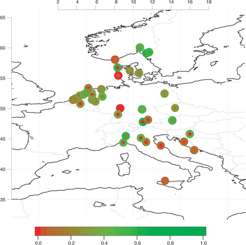
The two annual mean parameters describing the wet-day mean µ and frequency f _w were derived from daily rain gauge records taken from the climate archives of MET Norway (http://eklima.met.no) and from ECA&D (Klein Tank et al., 2002). The rain gauge records were selected based on the criteria that they included at least 130 yr, as long records were needed for the split-sample test. Figure 1 shows the location of the rain gauges. The 24-hour precipitation record from Bjørnholt in the forest north of Oslo was used as the primary data record. We let the capital letter X represent any random 24-hour precipitation, whereas the lower case symbol x is used to refer to a specific value. The exact definitions of µ and f _w are provided in the Appendix.

Fig. 1 The location of the rain gauge measurements for more than 130 yr. The size of the symbols is proportional to the number of valid data and their colour is according to the correlation between observed and predicted µ (inner part) or f _w (outer part) over the independent period.

2.2. Experiment design

Empirical orthogonal functions (EOFs) (Lorenz, 1956; North et al., 1982; Wilks, 1995; Benestad et al., 2008) can be used to represent the large-scale SAT and SLP conditions, here referred to as predictors. A third predictor e _s was derived from the SAT to represent the saturation vapour pressure according to the Clapeyron–Clausius equation (saturation evaporation pressure e _s =10^{(11.40–2353/T)} where T is temperature in degree Kelvin). The principal components (Strang, 1988) describe how the presence of the different large-scale EOF patterns vary over time, and were used as the independent variables (covariates) in an ordinary linear multiple regression. The regression involved a step-wise screening, based on the Akaike information criterion (Akaike, 1974). The regression-based ESD assumed that the data followed a normal distribution (see the Appendix).

The dependent variable in the regression represented the local precipitation statistics (µ and f _w ), and is referred to as predictand. Both predictors and predictands were aggregated on an annual basis for the calibration of the downscaling model. Both µ and f _w can be regarded as an estimate of the mean that, according to the central limit theorem, converges to a normal distribution with sample size (f _w is the mean of a series of zeroes and ones). We also checked how well µ and f _w conformed with the normal distribution though an analysis of the residuals. The precipitation data and the EOFs were also aggregated into seasonal and 5-yr (pentad) statistics respectively, to test whether a model trained on annual samples provided skilful predictions for smaller and larger samples. The purpose was to test the general validity of the model.

Common EOFs (Barnett, 1999; Benestad, 2001) were used for the model calibration to ensure that the seasonal and pentad EOFs corresponded to the same spatial patterns as the annual EOFs. The EOFs were computed independently for the large-scale atmospheric flow (SLP) and temperature anomalies (SAT), and the predictions were based on a step-wise approach where the ESD model first was calibrated on the e _s EOFs for the downscaling of the wet-day mean µ and the SAT EOFs for f _w respectively. The e _s or SAT-based regression model was then used to predict the local quantities, and the resulting residuals were then used to calibrate another regression model that used SLP EOFs as predictors. The final predictions based on both e _s /SAT and SLP were then synthesised by adding the predictions from the two steps. Limiting the EOFs to the first six leading ones imply both a selection of the largest spatial scales and reduces the risk of over-fit (Wilks, 1995), however, 12 EOFs were used for the locations other than Bjørnholt in order to improve the chances of finding a connection between local and large scales with a crude specification of predictor domain. A third step was introduced for the pentads to account for a possible link to the global mean temperature on the longer time scales (Benestad, 2013), where the residual of the downscaled pentad µ from the SAT and SLP EOFs was subject to a final regression against the global mean temperature as in Benestad (2013).

The experiments and analyses were designed for the evaluation of forecasts against independent data, and hence the ESD model used the interval 1900–1970 for calibration and independent data outside this interval for independent (out-of-sample) evaluation. The analysis was implemented in the R system for statistical computing (R Development Core Team, 2008, http://www.R-project.org/) and used the new R-package ‘esd’ (see the Appendix for more details).

2.3. Validation

The skill of the forecasts was assessed through the estimation of the Pearson correlation in the predicted and observed annual values µ and f _w . One reason for analysing annual mean values for these quantities is the expected characteristics of stochastic data of similar type: a normal distribution for the average of a continuous variable. Likewise, the skill of the predicted values for the annual wet-day 90th percentile q ₉₀ was assessed in terms of its correlation against corresponding quantity from the observations. The skill of predicted probabilities was assessed by comparing the annual observed number of events with precipitation exceeding a high threshold (10 mm/day) against a predicted 90% confidence interval, based on probability estimates and a binomial distribution. One diagnostic involved comparing the residual to Gaussian white noise (distribution shape, trend, and lagged correlation).

3. Results

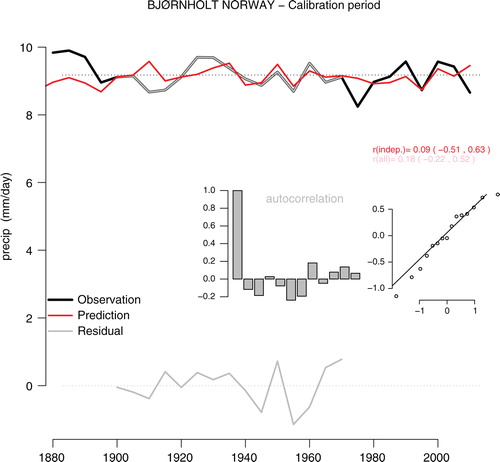
Figure 2 shows the downscaling results for the annual mean µ at Bjørnholt, which was the same data record as Benestad and Melsom (2002) found a teleconnection link in the North Atlantic. The upper part of the figure shows the observations and predictions. For the independent data, the correlation was 0.27 (with 90% confidence interval of 0.01–0.49), and for the entire period, the correlation was 0.38 (0.22–0.52). The predicted values in the calibration interval are shown in faint colours, and the residual is shown in the lower part of the figure. The inserted diagrams show the auto-correlation function (ACF) and the normal quantile–quantile plot (q–q normal) for the residuals. One indication that the analysis has identified all dependencies is when the residuals have low auto-correlation and are close to being normally distributed (white noise). Hence, these results suggest that the downscaling accounts for most of the connection to larger spatial scales. Table 1 (first column) shows similar scores for some European stations whose locations are shown in Fig. 1, where the colour scale of the inner part of the symbols indicates the correlations for µ. For a number of stations, the evaluation indicated no skill, however, there were also some stations with higher correlations, the highest being 0.42 for Strømsfoss sluse. Both the estimated and downscaled µ for Bjørnholt suggest a slight increase during the last evaluation period since 1960.

Fig. 2 An assessment of the downscaled µ. The upper part shows µ estimated from the rain gauge data (black) and predicted through the downscaling (red). The faint sections of the curves indicate the calibration interval. The correlation for the independent sections of the data are 0.27 the out-of-sample years and 0.38 for the entire curve, both statistically significant at the 5%-level. The lower part of the figure shows the residuals in grey, and the inserts show the auto-correlation function (ACF) and a q–q plot of the residuals against a normal distribution. The ACF indicates no persistence and the q–q plot suggest that the residuals follow the normal distribution closely.

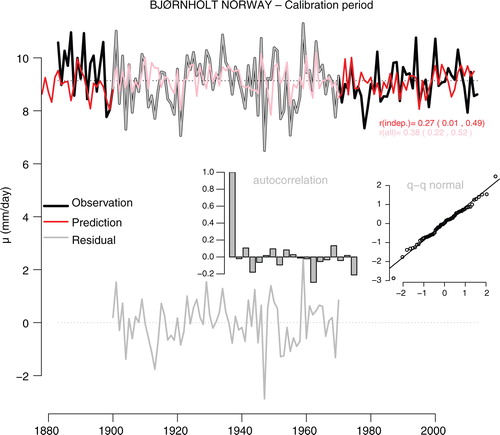
Table 1. Summary of correlation scores: Annual (both for the independent out-of-sample and for all years), seasonal and pentads of wet-day mean (µ) of precipitation

	Annual (ind.)	Annual (all)	q 90	DJF	MAM	JJA	SON	Pentads
BJØRNHOLT	0.27	0.38	0.28	0.15	0.25	0.29	0.39	0.18
BAMBERG	0.33	0.41	0.30	0.11	0.16	0.23	0.13	0.57
BERLIN-DAHLEM	0.25	0.25	0.17	0.23	−0.08	0.14	0.06	0.33
BOLOGNA	−0.02	0.07	0.11	0.11	0.04	−0.04	−0.13	−0.29
FRANKFURT	−0.04	0.15	0.12	0.05	0.00	0.09	0.07	0.29
GENOA	0.01	0.24	0.27	0.24	0.07	−0.07	0.13	−0.05
GOSPIC	0.02	0.08	0.10	0.01	0.03	−0.02	−0.08	0.37
GRONBAEK-ALLINGSKOVGARD	0.35	0.21	0.18	0.01	0.13	0.10	0.01	0.26
GRONINGEN-1	0.32	0.52	0.42	0.08	0.09	0.43	0.13	0.76
HALDEN	0.00	0.21	0.13	0.38	0.18	0.08	0.12	−0.07
HELMOND	0.28	0.39	0.32	0.08	0.17	0.29	0.19	0.25
HOHENPEISSENBERG	−0.06	0.09	0.15	−0.06	0.00	0.02	0.03	−0.19
HOOFDDORP	0.13	0.12	0.09	0.13	0.08	0.27	0.09	0.06
HOORN	0.06	0.21	0.15	0.20	0.11	0.33	0.15	0.19
HVAR	0.07	0.09	0.01	0.11	0.05	0.06	−0.07	NA
KARLSRUHE	−0.04	0.10	0.11	−0.07	0.14	0.06	0.08	0.14
KERKWERVE	0.32	0.35	0.33	0.16	0.02	0.32	0.18	0.62
KREMSMUENSTER	0.23	0.40	0.28	0.13	0.27	0.25	0.09	0.11
MANTOVA	−0.27	0.07	0.06	0.02	0.11	0.11	0.20	NA
MILAN	0.18	0.36	0.30	0.04	0.04	0.18	0.27	NA
MUENCHEN	−0.08	0.02	0.00	0.11	0.10	−0.09	−0.07	−0.35
NORDBY (FANO)	0.06	0.04	−0.06	0.18	0.13	−0.04	0.16	0.03
OKSOEY FYR	0.09	0.26	0.24	0.26	0.01	0.15	−0.10	0.34
PALERMO	0.14	0.41	0.32	0.24	0.15	−0.05	0.21	NA
PESARO	−0.12	0.06	0.04	−0.09	0.07	−0.05	0.13	NA
PRAHA-KLEMENTINUM	0.08	0.17	0.04	−0.23	−0.11	0.07	0.09	NA
PUTTEN (GLD)	−0.12	0.26	0.29	0.12	0.15	0.33	0.06	0.43
ROERMOND	0.06	0.28	0.29	0.01	0.16	0.22	0.12	0.35
SCHEVENINGEN	0.01	0.16	0.20	−0.15	0.11	0.16	0.02	0.08
STRØMSFOSS SLUSE	0.42	0.36	0.27	0.04	0.04	0.19	0.18	0.37
TRANEBJERG	0.19	0.40	0.31	0.36	0.18	0.24	0.04	0.52
UCCLE	−0.20	0.11	0.03	0.29	0.03	0.10	0.12	−0.12
VESTERVIG	−0.12	0.15	0.07	0.20	0.18	0.20	−0.02	−0.15
VLISSINGEN-1	0.04	0.18	0.16	0.09	−0.08	0.26	0.29	0.23
WEST TERSCHELLING	−0.09	0.37	0.26	0.33	0.15	0.25	0.00	0.30
WINTERSWIJK	0.14	0.38	0.30	0.13	0.11	−0.02	0.16	0.35
ZAGREB-GRIC	−0.02	0.14	0.15	0.17	0.08	−0.09	0.15	−0.18

The column ‘q ₉₀’ provides the correlation scores for the predicted q ₉₀ as in Fig. 8. The correlations for the seasons and pentads were for all years.

Figure 3 shows the results from a similar analysis as in Fig. 1, but for f _w rather than µ. The correlation between predicted and observed annual wet-day frequency was 0.48 for the out-of-sample data, with a 90% confidence interval of 0.26–0.66. Hence the results were statistically significant at the 5%-level. The ACF gave no indication of persistence in the residual and the qq-plot showed that the residuals were close to being normally distributed. However, the residual had a number of pronounced jumps (‘spikes’) between intervals where the values varied to a much smaller degree and with a somewhat more persistent character. Again, the inspection of the residual suggests that the downscaling captured most of the large-scale dependency in f _w . Since 1970, both the estimated and downscaled f _w suggest a slight increase, in other words, there has been more rainy days. The first column in Table 2 indicates that the correlations for f _w were in general higher than for µ, often exceeding 0.50. The skill scores for f _w are indicated by the colour of the outer circle of the symbols in Fig. 1. The highest score was 0.63 for Halden and Hohenpeissenberg.

Fig. 3 Same as Fig. 2 but for f _w . The correlation between the downscaled results and observed wet-day frequency is 0.48 (0.56 for the entire record) and statistically significant at the 5%-level. The two curves follow closely, albeit with periods of poorer match such as in the 1890s and 1990s. The residuals do not indicate the presence of persistence and appear to follow the normal distribution closely. Similar correlations for independent and the entire record suggest robust results.

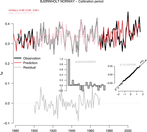
Table 2. Summary of correlation scores. Annual, seasonal and pentads of wet-day frequency (f _w ) of precipitation

	Annual (ind.)	Annual (all)	n (X>10 mm)	DJF	MAM	JJA	SON	Pentads
BJØRNHOLT	0.48	0.56	0.59	0.67	0.64	0.55	0.76	0.61
BAMBERG	0.51	0.57	0.46	0.49	0.48	0.23	0.66	0.41
BERLIN-DAHLEM	0.31	0.33	0.23	0.33	0.28	0.24	0.38	0.18
BOLOGNA	0.23	0.46	0.28	0.47	0.37	0.14	0.42	0.65
FRANKFURT	−0.10	0.18	0.16	0.13	0.10	0.07	0.51	0.19
GENOA	0.48	0.63	0.28	0.55	0.47	0.26	0.72	0.44
GOSPIC	0.11	0.40	0.41	0.30	0.38	0.28	0.36	0.32
GRONBAEK-ALLINGSKOVGARD	0.21	0.01	0.04	0.34	0.00	−0.29	0.21	0.13
GRONINGEN-1	0.26	0.44	0.30	0.69	0.66	0.40	0.66	−0.05
HALDEN	0.63	0.60	0.44	0.40	0.58	0.37	0.72	0.09
HELMOND	0.30	0.47	0.40	0.67	0.55	0.37	0.66	−0.03
HOHENPEISSENBERG	0.63	0.65	0.16	0.63	0.44	0.32	0.72	0.31
HOOFDDORP	0.45	0.57	0.23	0.62	0.74	0.48	0.70	0.21
HOORN	0.55	0.62	0.28	0.77	0.63	0.46	0.66	0.42
HVAR	0.11	0.50	0.44	0.50	0.31	0.24	0.34	0.67
KARLSRUHE	0.36	0.40	0.26	0.48	0.39	0.40	0.60	0.27
KERKWERVE	0.25	0.36	0.35	0.66	0.59	0.40	0.67	−0.29
KREMSMUENSTER	0.52	0.63	0.33	0.64	0.58	0.36	0.60	0.39
MANTOVA	0.42	0.57	0.20	0.48	0.51	0.13	0.52	NA
MILAN	0.59	0.71	0.44	0.52	0.54	0.35	0.62	NA
MUENCHEN	0.19	0.30	0.10	0.47	0.29	0.31	0.46	0.22
NORDBY (FANO)	−0.06	−0.07	0.10	−0.41	−0.14	−0.16	−0.06	−0.03
OKSOEY FYR	0.04	0.33	0.20	0.16	0.47	0.38	0.29	0.33
PALERMO	0.06	0.20	0.21	0.35	0.23	0.26	0.24	NA
PESARO	0.10	0.32	0.26	0.52	0.33	0.13	0.40	NA
PRAHA-KLEMENTINUM	0.30	0.27	0.02	0.13	0.24	0.14	0.15	NA
PUTTEN (GLD)	0.32	0.48	0.34	0.62	0.55	0.51	0.65	0.14
ROERMOND	0.29	0.41	0.28	0.55	0.52	0.30	0.66	−0.08
SCHEVENINGEN	0.30	0.49	0.35	0.61	0.55	0.47	0.66	0.11
STRØMSFOSS SLUSE	0.41	0.52	0.44	0.54	0.57	0.46	0.68	0.16
TRANEBJERG	0.29	0.50	0.35	0.62	0.54	0.60	0.64	0.39
UCCLE	0.28	0.56	0.29	0.61	0.56	0.61	0.74	0.24
VESTERVIG	0.56	0.60	0.30	0.76	0.63	0.60	0.79	−0.05
VLISSINGEN-1	0.21	0.38	0.21	0.49	0.59	0.48	0.62	−0.13
WEST TERSCHELLING	0.23	0.41	0.34	0.65	0.60	0.57	0.69	−0.10
WINTERSWIJK	0.46	0.53	0.38	0.67	0.59	0.42	0.64	−0.07
ZAGREB-GRIC	0.47	0.60	0.40	0.57	0.36	0.28	0.59	0.62

The column ‘n(X>10mm)’ shows the correlation between the median number of days with rainfall greater than 10 mm/day as in Fig. 9. There was a bias for some stations that gave a shift in the predicted 90% confidence interval even with moderately high correlations. The correlations for the seasons and pentads were for all years.

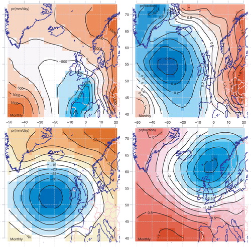
Figure 4 shows a set of maps indicating the regional patterns in surface temperature (upper) and mean sea-level pressure (lower) associated with high values for µ (left) and f _w (right) at Bjørnholt. The teleconnection patterns associated with µ exhibited a temperature gradient with cold conditions over the British Isles and the Bay of Biscay and warm conditions over northern Norway. The corresponding pattern for the SLP was characterised by low pressure to the west of the British Isles. However, the patterns associated with high frequency of wet days differed from those related to high amounts: cold conditions south of Greenland and west of Britain and warm over the central–northern European continent.

Fig. 4 Maps showing the spatial SAT (upper) and SLP (lower) anomalies associated with variations in µ (left) and f _w (right).

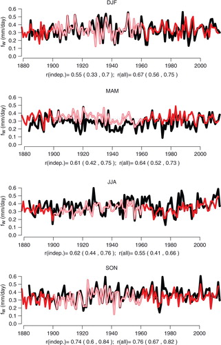
Figures 2–4 presented results for annual statistics. One interesting question is whether models calibrated on annual samples of µ can be used to predict variations on seasonal time scales. In this case, the definition of ‘independent’ was the seasons for the years which were not used for the calibration, and category ‘all’ also included the seasons for those years on which the annual aggregates were calibrated. Here we report the skills for all years, since the seasonal aggregates for the calibration period were not used to train the model. Figure 5 shows the results of such a test, however, the predictions for the seasons had little skill for µ during winter (0.15), but higher correlations for spring, summer and autumn (0.25, 0.29, 0.39, respectively; Table 1). Seasonal differences have also been noted in earlier studies (Wilby and Wigley, 2000; Hanssen-Bauer et al., 2003). One difference between the winter and the other seasons is that more of the precipitation is in the form of snow. The predicted values were slightly biased with respect to the observations and did not capture the peaks, but there were only minor differences between the mean levels during the different seasons. Table 1 suggests that findings for Bjørnholt of generally low-to-moderate seasonal correlation skills for µ (columns 4–7) and high for f _w (Table 2) are also fairly typical for the other European stations. A similar analysis for f _w (Fig. 6) suggested even higher scores. Downscaling calibrated for the annual mean f _w at Bjørnholt gave a correlation of 0.67 for winter, 0.64 for spring, 0.55 for the summer, and 0.76 for the autumn season.

Fig. 5 A comparison between seasonal µ for the four seasons and corresponding values predicted through the downscaling (red). The section of curves with faint colours indicate the calibration period. The correlation is distinguishable from zero only in summer. The results do not indicate that a model calibrated on annual data is valid for sub-annual time scales. Similar correlations for independent and the entire record suggest robust results.

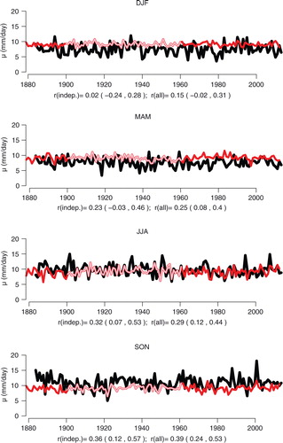
Fig. 6 A comparison between seasonal f _w for the four seasons and corresponding values predicted through the downscaling (red). The section of curves with faint colours indicate the calibration period. The correlation is distinguishable from zero only in summer. The results indicate that a model calibrated on annual data is valid for sub-annual time scales. Similar correlations for independent and the entire record suggest robust results.

For the pentads (5-yr aggregated values), the correlation between predictions of µ and the wet-day mean derived from the observations was 0.18 for all years (−0.22,+0.25) and not statistically significant (Fig. 7). It is worth bearing in mind that the number of data points in the correlation analysis was lower than for the annual analysis and makes a difference in the estimation of the confidence intervals. The ACF gave no indication of persistence in the residual, but rather a slight lag-one anti-correlation. The qq-plot for the residuals after the regression analysis against the (regional) air surface temperature and mean SLP showed a divergence from the diagonal in the lower tail. The lack of skill on the 5-yr timescale was fairly typical for those sites with sufficient record lengths (Table 2; last column). Similar exercise for f _w rather than µ indicated a reduction in the skill for the wet-day frequency on the 5-yr timescales (Table 2; last column).

Fig. 7 Same as Fig. 2 but for pentads. The residual does not suggest any persistence and is close to being normally distributed, after a third regression against the global mean temperature was included. There is a modest correlation between the predictions and observations, but the results do not indicate that a model calibrated on annual data is valid for multi-annual time scales.

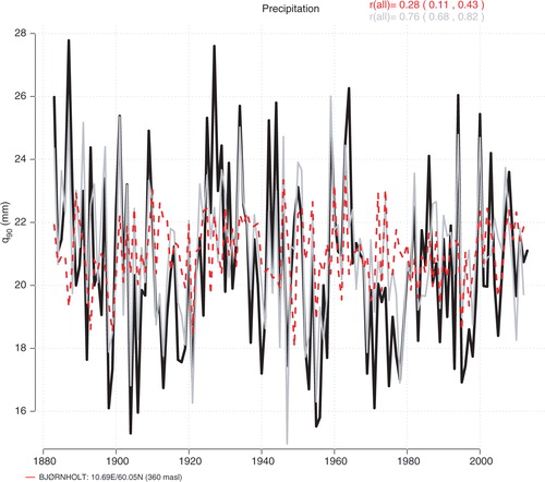
Figure 8 shows a comparison between the annual wet-day 90th percentile q ₉₀ from the observations, the corresponding values estimated from µ assuming an exponential distribution, and ${\hat{q}}_{90}$ predicted from SAT and SLP. The latter prediction took µ from Fig. 2 and solved for ${\hat{q}}_{90}=-ln(1-p)\mu (SAT,SLP)$. The year-to-year correlation between the downscaled and observed values was 0.28, and statistically significant at the 5%-level. In particular, the downscaling did not capture the magnitude of the major peaks in q ₉₀; however, the value of q ₉₀ derived directly from the observed µ gave a closer reproduction of the multiyear variations (grey; correlation of 0.76). The q ₉₀ was chosen rather than q ₉₅, as the former was less influenced by statistical fluctuations (f _w ~0.3 gives about 120 data points per year) and the annual q ₉₅ was strongly affected by a single year. In Table 1, the corresponding correlations are presented for the other European stations (column 3), and the general picture was a moderate and positive correlation between downscaled and observed q ₉₀.

Fig. 8 A comparison between observed wet-day 95-percentile q ₉₅ and corresponding values estimated from µ (grey) and through downscaling (red) using SAT and SLP as predictors. The method appears to capture some of the multiyear variations but not some of the most pronounced the individual spikes.

One way to use the downscaled results for forecasting is to estimate the number of events exceeding a certain threshold value each year. The method predicts the probability Pr(X>x ₀) based on the exponential distribution and f _w , and the confidence interval for the number of events can be estimated according to the binomial distribution (see the Appendix). For each year, a 90% confidence interval for the predicted number of events was estimated according to the predicted probability, which was compared with the observed number of events (henceforth ‘counts’). We would expect some of the counts to fall outside the confidence interval even if the predicted and observed data have an identical distribution, and the sum of the number of years out of a total of N years with the observed counts outside the predicted interval (${\hat{n}}_{05}(t)$–${\hat{n}}_{95}(t)$) is also expected to follow a binomial distribution for perfect predictions. Figure 9 shows a comparison between predicted number of precipitation events exceeding 10 mm/day [a threshold used by road authorities in Norway (Frauenfelder et al., 2013)] and the counts of observed events. 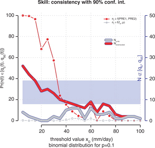The downscaled results reproduced the realistic multiyear variability with a correlation between the predicted annual median count n _m (t) and observed count n _o (t) of 0.6. However, the probability that the predictions conformed to the same statistical distribution as the 130 yr record was only 1% (i.e. different at the 5% statistical significance level). The predicted counts were outside the confidence interval in 22 of 130 yr, compared to a 90% confidence interval of 8–19 according to the binomial distribution. In other words, the predicted annual count of annual heavy-precipitation events based on the downscaling exhibited a wider distribution than the observed statistics with a high proportion of values outside the 90% confidence interval (p=1%). On the other hand, the same analysis applied to the annual wet-day means and frequencies taken directly from the observations suggested a narrower distribution and gave only two cases with counts outside the 90% confidence interval, significantly lower than expected (8–19). The assessment of skill should span over a range of threshold values, as shown in Fig. 10, displaying the probability of N being anomalously high or low (thin lines with symbols) for a range of different thresholds (x-axis). For thresholds x ₀ in the range 20–75 mm/day, the predicted results suggested a good correspondence with a binomial distribution with p=0.1. The number of observed counts outside the predicted 90% confidence interval (axis on the right), however, suggests that the value estimated from the observed annual mean µ and f _w was almost always within this range, and hence, the estimated confidence intervals were too wide (the predictions were ‘under-confident’), with the exception of low threshold values (x ₀<10mm/day).

Fig. 9 Predicted and observed number of intense precipitation events, defined by exceeding the threshold value x ₀=10mm/day. Symbols represent the counted events based on rain gauge data, grey shading the 90% confidence interval implied by µ and f _w derived from the observations, and red shading the 90% confidence interval derived through the downscaling exercise. The confidence intervals were derived taking the 5 and 95% percentiles from a binomial distribution where the probability for exceeding the 10 mm/day was taken from eq. (A4). The filled symbols mark the years when the number of events was outside the 90% confidence interval.

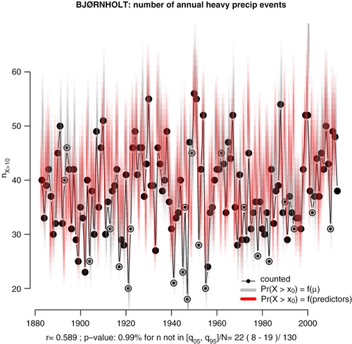
Fig. 10 A measure of skill. The right axis and the thick line indicate the number of observed events that were outside the predicted 90% confidence interval for a range of different threshold values x ₀ (x-axis). The left axis and thin lines indicate the probability associated with the observed number of intense wet events outside the predicted 5–95% annual interval estimated according to a binomial distribution. The number of years with events outside the confidence interval are counted and then the probability is estimated according to the binomial distribution, the sample size (number of years), and a probability of 10% for being outside the predicted 90% confidence interval. The red curves show results from the downscaling exercise whereas the grey curves show the results derived from µ and f _w estimated directly from the rain gauge data.

4. Discussion

The intention here was to emphasise the wet-day mean, as it is related to the statistics for variables that approximately follow an exponential distribution. Another point was to link the downscaled wet-day mean and frequency to the higher-order statistics, such as quantiles, number of days with heavy precipitation, and probabilities of exceedance.

One explanation why the correlation skill for q ₉₀ was lower than for n(X>10mm/day) may be that the latter was derived from both f _w and µ, that $Pr(X>x_0)\propto f_w$, and that the downscaling of f _w was associated with fairly good skill. The estimate of µ also provided a reasonable approximation for the shape of the pdf on which the results were based. A simple test was carried out where either µ or f _w were constant and set to their mean value respectively (see the supporting material). The results of this test suggested that both µ and f _w contribute to the estimate of the probability, but that f _w has a stronger influence on the results.

Another interesting question is why µ seems to be more difficult to predict than f _w . It was in general more difficult to establish a link between the large-scale climate conditions and local µ, and the skill scores for µ were low for a number of locations in Europe despite generally good results for f _w . Figure 1 showed no clear geographical pattern regarding the skill scores for µ, which is consistent with a high sensitivity to local conditions or a complex dependency where the amounts depend on several factors not accounted for. A principal component analysis (PCA) of annual variations in µ supports the notion of a weak dependency to large-scale conditions across the European stations (Benestad, 2013), as does the contrast with a PCA on annual f _w (supporting material). A canonical correlation analysis (Wilks, 1995) also suggests a more homogeneous spatial pattern in f _w than in µ. The scores for f _w in Fig. 1 also suggest generally good results in the north and reduced skill in the south and around the Mediterranean. Figure A2 in the supporting material shows a similar analysis as in Fig. 1 but for all years, and the inclusion of the dependent data clearly improves the scores. Both non-stationarity and varying data quality with time (Wijngaard et al., 2003) may explain some of these differences.

The physical processes and conditions involved differ for µ and f _w (Linderson et al., 2004), where µ is expected to bear the signature of the cloud microphysics and may be more strongly influenced by summer-time convection and associated temporal and spatial scales. A plausible physical picture is that the connection to large-scales involves mechanisms through which humidity is advected with a geostrophic flow caused by pressure differences. Another factor is the dependency of the rate of evaporation on the surface temperatures, with increased evaporation due to higher temperatures in accordance to the Clapeyron–Clausius equation. In addition, large-scale temperature gradients can affect the baroclinic stability and hence the genesis as well as the course of low-pressure systems, often associated with precipitation.

If higher µ in summer were due to more convective events, then the results for Bjørnholt may suggest that it may to some extent be possible to predict the aggregated values for µ from large-scale temperatures, vertical stability, or humidity. Another question is whether the low skill for µ for Bjørnholt in winter can be attributed to more snow and less liquid rain, for instance under-catch (Wolff et al., 2014). Another explanation is that low values of µ during winter means that the calibration with its annually aggregated value emphasises the warmer seasons with typically higher values. The predictor map for µ (Fig. 4; left panels) suggests that the higher values of the wet-day mean at Bjørnholt were associated with a low-pressure system over the British Isles and a southwest–northeast temperature gradient.

The corresponding results for the other stations gave a mixed picture, with some locations exhibiting similar scores as for Bjørnholt (green symbols in Fig. 1) whereas others indicated low skill (red symbols in Fig. 1). There may be several reasons for the geographical variations in skill, such as the use of a fixed predictor domain size and the different locations being exposed to different prevailing winds and weather types. Another reason may be that the ECA&D data set is not homogeneous (Wijngaard et al., 2003). Furthermore, the experimental set-up may not have sufficiently captured the geographic variations in the link between small and large scales, and including 12 EOFs is associated with a higher risk for over-fit than including only six.

The marginal distribution for 24-hour precipitation tends to have a fat tail compared to that of the exponential distribution (Benestad et al., 2012a, 2012b), and hence the exponential distribution will tend to under-estimate the probabilities associated with extreme precipitation. More accurate results are obtained with proper EVT (Coles, 1999). The Appendix provides a crude comparison between return-values derived based on EVT and the framework based on the exponential distribution presented in this paper. If the imprecision associated with the latter is acceptable, then crude estimates for daily precipitation return periods can be derived from downscaled results for µ and f _w .

It is also questionable whether the 20 C reanalysis used in these ‘perfect predictor experiments’ provide a sufficient representation of the past SAT and SLP. Changes in the surface network of observations may have an effect on its degree of homogeneity, and the lack of upper-air observations and imperfect estimates of historical sea surface temperatures imply that the reanalysis has some limitations. We have not addressed those here, but such caveats mean that the analysis presented here is not quite equal to ‘perfect predictor experiments’.

Different experiments can shed light on processes connecting the large-scale conditions and the local rainfall statistics, such as ‘pseudo-reality’-based ones. Such a study is beyond the scope of this paper, which addresses the question whether we can make actually useful forecasts of precipitation statistics seasons to decades ahead, given large-scale patterns in surface temperature and mean SLP. A ‘pseudo-reality’ set-up could also by-pass problems such as imperfections in the reanalysis data.

A concern for seasonal-to-decadal forecasting is whether GCMs are able to skilfully forecast the large-scale patterns in SAT and SLP over the North-Atlantic on a seasonal-to-decadal time scales, and the greatest bottle neck in terms of providing such forecasts for the North-Atlantic region seems to be due to the limited understanding of the role of various physical processes, the presence of complex chaos, and whether the GCMs actually capture crucial precursory signals. The coarse spatial resolution in the ocean models used in the GCMs may limit their ability to adequately represent ocean currents and associated heat transport. Furthermore, Benestad et al. (2010) carried out a number of simulations with different Arctic sea-ice conditions and found that the temperature response was pronounced for Europe but not systematic, suggesting a strong presence of non-linearities. European teleconnection mechanisms may involve dynamical processes which are hard to forecast, such as the Arctic vortex, the NAO, jet streams, and storm tracks. The roles of oceanic heat distribution and currents are still not well known. In this study, the same predictor set-up was used for all the European stations, however, the skill will probably be higher for some locations with a different predictor choice. Seasonal forecasts tend to have more skill in the Tropics, e.g. for the ENSO, and the same methods used here may provide useful estimates of probabilities for heavy rainfall seasons ahead.

5. Conclusions

We show how ESD can be applied to parameters that traditionally have not been commonly used in downscaling, such as predicting probabilities and number of intense precipitation events. Furthermore, we provide a contribution to a more ‘comprehensive evaluation’ (Murphy et al., 2010) to measure the compound effect of downscaling biases in terms of the number of events predicted over time. However, we do not attempt to assess the compound skill of GCM and downscaling here.

The results presented here suggest that it is possible to estimate local precipitation statistics with some predictive skill given large scale SAT and SLP conditions. The wet-day frequency in particular seems to bear a strong dependency to the large-scale atmospheric conditions, although a weak link was also found for the wet-day mean µ which is a proxy for the precipitation amount. A prediction of precipitation statistics on seasonal-to-decadal time scales based on these results will be probabilistic with approximate estimates, and hence the presence of uncertainties will linger on. The precipitation amount (µ) was sensitive to time scale in certain circumstances and hence sample size. A possible reason for this may be the presence of different physical processes with different intrinsic time scales, most likely in the large-scale predictors and seasonal differences between processes producing rain and snow. Hence, the different time scales in the predictors and the predictands may reflect different physical processes in terms of the rainfall amount on a wet day. The weak skill for winter may also be due to the generally low precipitation amounts during winter and that the annual wet-day mean emphasises the season with higher rainfall. The wet-day frequency was generally not sensitive to seasonal or annual time scales, which may suggest that similar physical mechanisms responsible for the wet-dry occurrence is present on seasonal and annual time scales. The analysis for 5-yr time scales failed to find dependencies between large and small scales for the chosen predictors. The results suggest that models calibrated on annual data samples may in some cases provide skilful forecasts on seasonal time scales only.

6. Acknowledgements

This work has been supported by the Norwegian Meteorological Institute and SPECS (EU Grant Agreement 3038378). We also like to thank Reidun Gangstø, Inger Hanssen-Bauer and Oskar Andreas Landgren for reading and commenting on the manuscript.

Notes

To access the supplementary material to this article, please see Supplementary files under ‘Article Tools’.

7. Appendix

Definitions

The wet-day mean is the mean value of all days where the amounts exceed the threshold value x ₀=1mm/day:A1 $\mu =\sum _{i=1}^N(x)/n_w;\forall x>x_0,$A1

where N is the rain gauge sample size (number of days) and the total number of wet days is $n_w=\sum _{i=1}^N\mathrm{\mathscr{H}}(x_i>x_0)$ where $\mathrm{\mathscr{H}}$ is the Heaviside function. The wet-day frequency is the number of days where the amounts exceed the threshold value x ₀=1mm/day divided by the total number of days:A2 $f_w=\sum _{i=1}^N\mathrm{\mathscr{H}}(x>x_0)/N$A2

Method in detail

Daily precipitation data were sorted into wet (X>1mm/day) and dry days as in Benestad et al. (2012a, 2012b) and Benestad (2013), where the precipitation statistics were characterised by the annual wet-day mean µ and the annual wet-day frequency f _w . The ordinary all-day mean precipitation is the product of the wet-day frequency and mean $\overline{x}=f_w\mu$.

The wet-day 24-hour precipitation was taken to be approximately exponentially distributed, whereas the variable describing a wet or a dry day was expected to follow a binomial distribution (o∈[0,1]). In contrary to the variables, statistical parameters describing the annual mean wet-day mean µ and the annual mean wet-day frequency f _w follow a normal distribution according to the central limit theorem (Wheelan, 2014), as seen in the qq-plots in Figs. 2 and 3. The design of the experiment where regression analysis was applied to annually aggregated statistics was motivated by the convenience of an expected normal distribution according to the central limit theorem.

The experiments used regression-based ESD, involving step-wise screening applied to the principal components describing the EOFs, and the regression model used in the ESD wasA3 $\mu (t)={\beta }_0+\sum _{i=1}^m({\beta }_i{x}_{SAT}{(t)}_i)+\mathrm{\epsilon },$A3

where x _SAT (t) refers to the principal components associated with the EOFs describing the annual mean SAT, and ɛ is an error term describing the residual. Equation A3 was repeated after µ was replaced by the residual ɛ and x _SAT (t) with the principal components describing the SLP (x _SLP (t)) and the final downscaled results were the sum of the two steps.

On a separate account, we wanted to examine the possibility to predict reliable probabilities for extreme precipitation events, given a skilful prediction of µ and based on the prediction of pdfs for 24-hour precipitation. Let the 24-hour precipitation be approximately represented by an exponential distribution,A4 $Pr(X<x)={\int }_0^{\infty }\lambda e^{-\lambda x}dx=(1-e^{-\lambda x}),$A4

for which the mean value is $\mu =1/\lambda$ and variance ${\sigma }^2=1/{\lambda }^2={\mu }^2$. If the wet-day precipitation follows an exponential distribution, then any quantile q _p is directly specified in terms of the wet-day mean µ:A5 $q_p=-ln(1-p)\mu .$A5

We also can solve for the value of any return value $x_{\tau }$ analytically if we know the fraction of wet days f _w and the data actually follows an exponential distribution (we know that this is not the case here, as the tail is thicker than for the exponential distribution):A6 $\frac{1}{\tau }=f_{w}Pr(X>x_{\tau })=f_w{e}^{-x_{\tau }/\mu },$A6

therefore,A7 $x_{\tau }=-ln(\frac{1}{\tau f_w})\mu .$A7

We can then estimate the probability of exceedance $X>x_{\tau }$ for a year and the number of events according to a binomial distribution. We let the probability for an event $X>x_{\tau }$ be $p=f_w{e}^{-x_{\tau }/\mu }$, and use the binomial distribution to estimate the number of events k estimated for a given interval with length n: $C_n^k{p}^k{(1-p)}^{(n-k)}$.

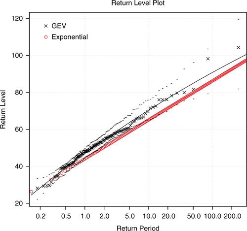
It is possible to compare $x_{\tau }$ from the equation above with the return values estimated from proper EVT using general extreme value distribution (GEV) (Coles, 1999) (Fig. A1). The return values for Bjørnholt was estimated using the R-package ‘evd’ and fgev which subsequently were compared with $x_{\tau }$.

Fig. A1 A comparison between return values derived from GEV and eq. (A6) for Bjørnholt suggests that the exponential distribution has a tendency to under-estimate the return-levels. Still, the ‘error’ associated with the estimates based on the simpler expression for $x_{\tau }$ are less than 10% compared with the GEV-based estimates (not shown). Hence, a rough estimate for return-levels can be obtained by downscaling the wet-day mean µ and frequency f _w .

The R-package ‘esd’

The wet-day mean µ and frequency f _w were derived from a set of methods provided by the R-package ‘esd’ (Benestad et al., 2014) developed under the R core programming tool (R Core Team, 2014):$\text{mu}<-\text{as}.\text{annual}(\text{y},\text{FUN}=\text{'}\text{exceedance}\text{'},\text{threshold}=\text{threshold})\text{fw}<-\text{as}.\text{annual}(\text{y},\text{FUN}=\text{'}\text{wetfreq}\text{'},\text{threshold}=\text{threshold})$

The ‘esd’ package is made freely available by the Norwegian Meteorological Institute (MET Norway) and is for use by the climate community. It was primarily built for statistical downscaling of climate variables and parameters from global (e.g. ENSEMBLES, CMIP3/5 model results) and/or regional climate models (EURO-CORDEX), and has recently been extended to deal with data I/O, statistical analysis and visualisation. It consists of (1) retrieving and manipulating large samples of climate and model data from various sources, and (2) computing Empirical Orthogonal Functions (EOFs), PCA, and Multi-Variate Regressions (MVRs) using very simple R commands and procedures (See R Script in the supporting material). The esd package has been built with the emphasis of traceability, compatibility, and transparency of the data, methods, procedures, and results. As the ‘esd’ package has been built on R system, it inherits from the large number of R built-in functions and procedures. Finally, it can be easily tailored to various climate analysis with few adaptations such as the one described in this paper.

An example of programming commands is described hereafter including a four-steps procedure. The first step consists of retrieving daily precipitation from the MET Norway archive using the function ‘station’ as the following$\text{y}<-\text{station}(\text{'}\text{precipitation}\text{'},\text{'}\text{met norway archive}\text{'})\}$

The second step consist of getting global climate model output and reanalysis data using the function ‘retrieve’ as the following$\text{gcm}<-\text{retrieve}(\text{'}\text{any global climate model}\text{'}>)\},\text{rea}<-\text{retrieve}(\text{'}\text{any reanalysis}\text{'})\}.$

The third step consists of computing the common EOFs using the function ‘EOF’ as follows$\text{ceof}<-\text{EOF}(\text{gcm},\text{rea})\}.$

Finally, the downscaling of y from the common EOF ‘ceof’ is achieved using the function ‘DS’ as the following$\text{ds}<-\text{DS}(\text{y},\text{eof})\}.$

References

- Akaike H . A new look at the statistical model identification. IEEE Trans. Automat. Contr. 1974; 19(6): 716–723.
- Baldwin M. P. , Dunkerton T. J . Stratospheric harbingers of anomalous weather regimes. Science. 2001; 294: 581–584.
- Baldwin M. P. , Stephenson D. B. , Thompson D. W. J. , Dunkerton T. J. , Charlton A. J. , co-authors . Stratospheric memory and skill of extended-range weather forecasts. Science. 2003; 301: 636–640.
- Barnett T. , Preisendorfer R . Origins and levels of monthly and seasonal forecast skill for United States surface air temperatures determined by canonical correlation analysis. Mon. Weather Rev. 1987; 115: 1825–1850.
- Barnett T. P . Comparison of near-surface air temperature variability in 11 coupled global climate models. J. Clim. 1999; 12: 511–518.
- Barnston A. G. , van den Dool H. M. , Zebiak S. E. , Barnett T. P. , Ji M. , co-authors . Long-lead seasonal forecasts – where do we stand?. Bull. Am. Meteorol. Soc. 1994; 75: 2097–2114.
- Barsugli J. J. , Guentchev G. , Horton R. M. , Wood A. , Mearns L. O. , co-authors . The practitioner's dilemma: how to assess the credibility of downscaled climate projections. Eos Trans. Am. Geophys. Union. 2013; 94(46): 424–425.
- Benestad R. , Nychka D. , Mearns L. O . Spatially and temporally consistent prediction of heavy precipitation from mean values. Nat. Clim. Change. 2012a; 2: 544–547.
- Benestad R. , Nychka D. , Mearns L. O . Specification of wet-day daily rainfall quantiles from the mean value. Tellus A. 2012b; 64: 14981.
- Benestad R. E . A comparison between two empirical downscaling strategies. Int. J. Climatol. 2001; 21: 1645–1668.
- Benestad R. E . Association between trends in daily rainfall percentiles and the global mean temperature. J. Geophys. Res. Atmos. 2013; 118(19): 10802–10810.
- Benestad R. E. , Hanssen-Bauer I. , Chen D . Empirical-Statistical Downscaling. 2008; Singapore: World Scientific.
- Benestad R. E. , Melsom A . Is there a link between the unusually wet autumns in southeastern Norway and SST anomalies?. Clim. Res. 2002; 23: 67–79.
- Benestad R. E., Mezghani A., Parding K. M. esd for Mac & Linux/esd for windows. figshare. 2014. Online at: http://figshare.com/articles/esd_for_Mac_amp_Linux/1160493.
- Benestad R. E. , Senan R. , Balmaseda M. , Ferranti L. , Orsolini Y. , co-authors . Sensitivity of summer 2-m temperature to sea ice conditions. Tellus A. 2010; 63: 324–337.
- Brönnimann S. , Luterbacher J. , Staehelin J. , Svendby T. M. , Hansen G. , co-authors . Extreme climate of the global troposphere and stratosphere in the 1940–42 related el Niño. Nature. 2004; 431: 971–974.
- Buishand T. A . Some remarks on the use of daily rainfall models. J. Hydrol. 1978; 36(3–4): 295–308.
- Burgueo A. , Martnez M. D. , Lana X. , Serra C . Statistical distributions of the daily rainfall regime in Catalonia (northeastern Spain) for the years 1950–2000. Int. J. Climatol. 2005; 25(10): 1381–1403.
- Cagnazzo C. , Manzini E . Impact of the stratosphere on the winter tropospheric teleconnections between ENSO and the north Atlantic and European region. J. Clim. 2009; 22: 1223–1238.
- Coles S. Extreme value theory and applications. Notes from a Course on EVT and Applications Presented at the 44th Reunio Annual da RBRAS e 8th SEAGRO. 1999; So Paulo, Brazil: Bucato. Online at: http://www.maths.bris.ac.uk/masgc/extremes/exnewnotes2.ps.
- Compo G. P. , Sardeshmukh P. D . Storm track predictability on seasonal and decadal scales. J. Clim. 2004; 17: 3701–3720.
- Compo G. P. , Whitaker J. S. , Sardeshmukh P. D. , Matsui N. , Allan R. J. , co-authors . The twentieth century reanalysis project. Q. J. Roy. Meteorol. Soc. 2011; 137(654): 1–28.
- Derome J. , Brunet G. , Plante A. , Gagnon N. , Boer G. J. , co-authors . Seasonal predictions based on two dynamical models. Atmos. Ocean. 2001; 39(4): 485–501.
- Derome J. , Lin H. , Brunet G . Seasonal forecasting with a simple general circulation model: predictive skill in the AO and PNA. J. Clim. 2005; 18: 597–611.
- Dix M. R. , Hunt B. G . Chaotic influences and the problem of deterministic seasonal predictions. Int. J. Climatol. 1995; 15(7): 729–752.
- Doblas-Reyes F. J. , Hagedorn R. , Palmer T. N . Developments in dynamical seasonal forecasting relevant to agricultural management. Clim. Res. 2007; 33: 19–26.
- Feddersen H . Predictability of seasonal precipitation in the Nordic region. Tellus A. 2003; 55: 385–400.
- Feddersen H. , Andersen U . A method for statistical downscaling of seasonal ensemble predictions. Tellus A. 2005; 57: 398–408.
- Frauenfelder R. , Solheim A. , Isaksen K. , Romstad B. , Dyrrdal A. V. , co-authors . Impacts of Extreme Weather Events on Infrastructure in Norway (InfraRisk). 2013; Oslo, Norway: Norges Geotekniske Institutt. Sluttrapport til NFR – prosjekt 200689 NGI rapport nr. 20091808.
- George S. E. , Sutton R. T . Predictability and skill of boreal winter forecasts made with the ECMWF seasonal forecast system II. Q. J. Roy. Meteorol. Soc. 2006; 132: 2031–2053.
- Gershunov A. , Barnett T. P . ENSO influence on intraseasonal extreme rainfall and temperature frequencies in the contiguous United States: observations and model results. J. Clim. 1998; 11: 1575–1586.
- Hanssen-Bauer I. , Frland E. J. , Haugen J. E. , Tveito O. E . Temperature and precipitation scenarios for Norway: comparison of results from dynamical and empirical downscaling. Clim. Res. 2003; 25: 15–27.
- Hawkins T. W. , Ellis A. W. , Skindlov J. A. , Reigle D . Inter-annual analysis of the North American snow cover-monsoon teleconnection: seasonal forecasting utility. J. Clim. 2002; 15: 1743–1753.
- Johansson Å . Prediction skill of the NAO and PNA from daily to seasonal time scales. J. Clim. 2007; 20: 1957–1975.
- Johansson Å. , Barnston A. , Saha S. , van den Dool H . On the level and origin of seasonal forecast skill in northern Europe. J. Atmos. Sci. 1998; 55: 103–127.
- Kharin V. V. , Zwiers F. W . Improved seasonal probability forecasts. J. Clim. 2003; 16: 1684–1701.
- Klein Tank A. J. B. W. , Können G. P. , Böhm R. , Demarée G. , Gocheva A. , co-authors . Daily dataset of 20th-century surface air temperature and precipitation series for the European climate assessment. Int. J. Climatol. 2002; 22: 1441–1453.
- Krishnamurti T. N. , Kishtawal C. M. , LaRow T. E. , Bachiochi D. R. , Zhang Z. , co-authors . Improved weather and seasonal climate forecasts from multimodel superensembles. Science. 1999; 285: 1548–1550.
- Landman W. A. , Kgatuke M.-J. , Mbedzi M. , Beraki A. , Bartman A. , co-authors . Performance comparison of some dynamical and empirical downscaling methods for South Africa from a seasonal climate modelling perspective. Int. J. Climatol. 2009; 29: 1535–1549.
- Li S. , Goddard L. , DeWitt D. G . Predictive skill of AGCM seasonal forecasts subject to different SST prediction methodologies. J. Clim. 2008; 21: 2169–2186.
- Linderson M.-L. , Achberger C. , Chen D . Statistical downscaling and scenario construction of precipitation in Scania, southern Sweden. Nord. Hydrol. 2004; 35: 261–278.
- Lloyd-Huges B. , Saunders M. A . Seasonal prediction of European spring precipitation from El Nino-southern oscillation and local sea-surface temperatures. Int. J. Climatol. 2002; 22: 1–14.
- Lorenz E. N . Empirical Orthogonal Functions and Statistical Weather Prediction. 1956; MIT, Cambridge, MA: Department of Meteorology. Scientific Report No. 1.
- Maraun D. , Widmann M. , Gutierrez J. , Kotlarski S. , Chandler R. , co-authors . Value – a framework to validate downscaling approaches for climate change studies. Earths Future. 2015; 3: 1–14.
- Murphy J. , Kattsov V. , Keenlyside N. , Kimoto M. , Meehl G. , co-authors . Towards prediction of decadal climate variability and change. Proc. Environ. Sci. 2010; 1: 287–304.
- North G. R. , Bell T. L. , Cahalan R. F . Sampling errors in the estimation of empirical orthogonal functions. Mon. Weather Rev. 1982; 110: 699–706.
- Orsolini Y. , Senan R. , Benestad R. E. , Melsom A . Autumn atmospheric response to the 2007 low Arctic sea ice extent in coupled ocean-atmosphere hindcasts. Clim. Dyn. 2011; 38: 2437–2448.
- Palmer T . Progress towards reliable and useful seasonal and interannual climate prediction. WMO Bull. 2004; 53: 325–333.
- Palmer T. , Alessandri A. , Andersen U. , Cantelaube P. , Davey M. , co-authors . Development of a European multi-model ensemble system for seasonal to inter-annual prediction (DEMETER). Bull. Am. Meteorol. Soc. 2004; 85: 853–872.
- Palmer T. , Anderson D . The prospect for seasonal forecasting – a review paper. Q. J. Roy. Meteorol. Soc. 1994; 120: 755–793.
- Palmer T. N. , Branckovic C. , Richardson D. S . A probability and decision-model analysis of PROVOST seasonal multi-model ensemble integrations. Q. J. Roy. Meteorol. Soc. 2000; 126: 2013–2034.
- R Core Team. R: A Language and Environment for Statistical Computing. 2014. R Core Team R Foundation for Statistical Computing, Vienna, Austria.
- Reason C. J. C. , Landman W. , Tennantc W . Seasonal to decadal prediction of southern African climate and its links with variability of the Atlantic ocean. Bull. Am. Meteorol. Soc. 2006; 87: 941–955.
- Rodwell M. J. , Doblas-Reyes F. J . Medium-range, monthly, and seasonal prediction for Europe and the use of forecast information. J. Clim. 2006; 19: 6025–6045.
- Stockdale T. N. , Anderson D. L. T. , Alves J. O. S. , Balmaseda M. A . Global seasonal rainfall forecasts using a coupled ocean-atmosphere model. Nature. 1998; 392: 370–373.
- Stocker T. F. , Qin D. , Plattner G.-K. , Tignor M. , Allen S.K. , co-authors . Climate change 2013: the physical science basis. Contribution of Working Group I to the Fifth Assessment Report of the Intergovern – Mental Panel on Climate Change. 2013; Cambridge, UK: Cambridge University Press.
- Strang G . Linear Algebra and its Application. 1988; San Diego, CA: Harcourt Brace & Company.
- Thom H. C. S . A note on the gamma distribution. Mon. Weather Rev. 1958; 86(4): 117–122.
- Thompson D. W. J. , Baldwin M. P. , Wallace J. M . Stratospheric connection to northern Hemisphere wintertime weather: implications for prediction. J. Clim. 2002; 15: 1421–1428.
- Ueda H. , Shinoda M. , Kamahori H . Spring northward retreat of Eurasian snow cover relevant to seasonal and interannual variations of atmospheric circulation. Int. J. Climatol. 2003; 23: 615–629.
- van der Linden P , Mitchell J. F. B . Ensembles: Climate Change and its Impacts: Summary of Research and Results from the ENSEMBLES Project European Commission. 2009; Exeter, UK: Met Office Hadley Centre.
- Vitard F. , Stockdale T. , Ferranti L . Seasonal forecasting of tropical storm frequency. ECMWF Newslett. 2007; 112: 16–22.
- Weigel A. P. , Liniger M. A. , Appenzeller C . Can multi-model combination really enhance the prediction skill of probabilistic ensemble forecasts?. Q. J. Roy. Meteorol. Soc. 2008; 134(630): 241–260.
- Wheelan C. J . Naked Statistics: Stripping the Dread from the Data. 2014; Newyork, NY: Met W. W. Norton & Company.
- Wijngaard J. B. , Tank A. M. G. K. , Können G. P . Homogeneity of 20th century daily temperature and precipitation series. Int. J. Climatol. 2003; 23: 679–692.
- Wilby R. , Wigley T . Precipitation predictors for downscaling: observed and general circulation model relationships. Int. J. Climatol. 2000; 20: 641–661.
- Wilby R. L. , Wigley T. M. L . Future changes in the distribution of daily precipitation totals across north America. Geophys. Res. Lett. 2002; 29(7): 39-1–39-4.
- Wilks D . Multisite generalization of a daily stochastic precipitation model. J. Hydrol. 1998; 210: 178–191.
- Wilks D. S . Statistical Methods in the Atmospheric Sciences. 1995; Orlando, FL: Academic Press.
- Wilks D. S . On “field significance” and the false discovery rate. J. Appl. Meteorol. Climatol. 2006; 45: 1181–1189.
- Wilks D. S. , Wilby R. L . The weather generation game: a review of stochastic weather models. Prog. Phys. Geogr. 1999; 23(3): 329–357.
- Wolff M. , Isaksen K. , Petersen-Øverleir A. , Ødemark K. , Reitan T. , co-authors . Derivation of a new continuous adjustment function for correcting wind-induced loss of solid precipitation: results of a Norwegian field study. Hydrol. Earth Syst. Sci. Discuss. 2014; 11: 10043–10084.
- Yun W. T. , Stefanova L. , Krishnamurti T. N . Improvement of the multimodel superensemble technique for seasonal forecasts. J. Clim. 2003; 16: 3834–3840.
- Zhang H. , Frederiksen C. S . Local and nonlocal impacts of soil moisture initialization on AGCM seasonal forecasts: a model sensitivity study. J. Clim. 2003; 16: 2117–2137.