Spectral analysis of forecast error investigated with an observing system simulation experiment

Abstract

The spectra of analysis and forecast error are examined using the observing system simulation experiment framework developed at the National Aeronautics and Space Administration Global Modeling and Assimilation Office. A global numerical weather prediction model, the Global Earth Observing System version 5 with Gridpoint Statistical Interpolation data assimilation, is cycled for 2 months with once-daily forecasts to 336 hours to generate a Control case. Verification of forecast errors using the nature run (NR) as truth is compared with verification of forecast errors using self-analysis; significant underestimation of forecast errors is seen using self-analysis verification for up to 48 hours. Likewise, self-analysis verification significantly overestimates the error growth rates of the early forecast, as well as mis-characterising the spatial scales at which the strongest growth occurs. The NR-verified error variances exhibit a complicated progression of growth, particularly for low wavenumber errors. In a second experiment, cycling of the model and data assimilation over the same period is repeated, but using synthetic observations with different explicitly added observation errors having the same error variances as the control experiment, thus creating a different realisation of the control. The forecast errors of the two experiments become more correlated during the early forecast period, with correlations increasing for up to 72 hours before beginning to decrease.

• numerical weather prediction
• OSSE
• error spectra
• GEOS-5 model
• nature run
• analysis verification

1. Introduction

The evolution of error growth in numerical weather prediction (NWP) from the analysis state to the extended forecast has been of interest since the early development of atmospheric models (Thompson, 1957; Lorenz, 1963, 1993; Charney et al., 1966; Smagorinsky, 1969). Understanding the nature of error growth helps provide guidance for the best methods of reducing forecast error, as well as quantification of the uncertainty of predictions. Previous studies of error growth have ranged from theoretical approaches (Leith and Kraichnan, 1972; Leith, 1974; Lorenz, 2011) and simplified and toy model investigations (Lorenz, 1963; Lorenz and Emanuel, 1998), to diagnostics of operational NWP systems (Lorenz, 1982; Simmons and Hollingsworth, 2002; Palmer and Hagedom, 2006).

Although it is desirable to investigate error growth with full-scale forecast models in order to retain the complexity of operational systems, there are some limitations to the use of standard output from NWP models. The greatest impediment to the study of analysis and short-term forecast errors in an operational system is the lack of a ‘truth’ for verification. In most cases, the analysis state has been generated using all available high-quality observations, so that there is no generally more reliable measure of the atmospheric state that could be used as truth to quantify the analysis error. However, the analysis itself has errors that are not significantly smaller than the magnitude of short-term forecast errors, resulting in difficulty characterising short-term forecast errors.

The short-term forecast error is of particular interest, as the background error estimate should be as accurate as possible to optimise the efficacy of the data assimilation system (DAS). Short-term forecast errors have been estimated by comparison of the model state with high-quality observational sets (e.g. Hollingsworth and Lonnberg, 1986; Andersson et al., 2000), but these studies are limited to cases where a reliable verification dataset is available.

Simple estimates of error variance often take the form of exponential growth (Lorenz, 1982) during the early forecast period, with error asymptoting to a saturation value at long forecast times (Leith, 1978) and an additional component of model error due to time independent or white noise. While early efforts such as Dalcher and Kalnay (1987) and Simmons et al. (1995) found that the model error term was not necessary to obtain a good fit of theory to actual forecast error for 500 hPa geopotential height, other studies (Savijärvi, 1995; Simmons and Hollingsworth, 2002) found that model error was required to make a close fit between theory and forecast error growth. These studies were not able to examine the growth of forecast errors prior to the 24-hour forecast time. Orrell et al. (2001) and Tribbia and Baumhefner (2004) employed ‘imperfect twin’ model experiments to explore the role of model error, but the model errors in these types of studies were relatively simple.

Relatively few investigations of forecast error spectra have been performed using operational NWP systems. Dalcher and Kalnay (1987) and Boer (1994) examined error spectra for the European Centre for Medium-Range Weather Forecasts (ECMWF) model, while Savijärvi (1995) investigated the National Meteorological Center Medium-Range Forecast (MRF) model and Boer (2003) evaluated error spectra of the Canadian Meteorological Centre (CMC) model. These studies were not able to calculate error spectra of the analysis or initial forecast period.

A tool that can be used to evaluate the errors in the very early forecast period is an observing system simulation experiment (OSSE). In an OSSE, the ‘truth’ is known in the form of a long, free-running model forecast called the nature run (NR). This NR replaces the actual atmosphere in the experiment, with all observations simulated from the NR fields and then assimilated into an NWP model analysis to produce a forecast. One major advantage of an OSSE is that the analysis and forecast errors may be explicitly calculated with respect to the NR. Another virtue of the OSSE framework is the ability to directly manipulate the qualities of the simulated observations, particularly the observation errors. Of course, this only provides useful information about the real problem in so far as the OSSE validates (Errico et al., 2013; Privé et al., 2013c).

The National Aeronautics and Space Administration Global Modeling and Assimilation Office (NASA/GMAO) has developed a global OSSE framework to support efforts to improve data assimilation techniques as well as for the development of new observing systems. The GMAO OSSE has been used to explore model error (Privé et al., 2013b) and observation error (Privé et al., 2013a), in both cases with a focus on forecasts of up to 120 hours. In the present study, the progression of error from the analysis state to the extended forecast is examined using the GMAO OSSE to explicitly calculate error. The spectral characteristics of the error are also evaluated as the forecast progresses.

The experimental method is given in Section 2, the results are described in Section 3 and the findings are discussed in Section 4.

2. Method

The GMAO global OSSE has been extensively calibrated as documented by Errico et al. (2013) and Privé et al. (2013c). The NR employed is a 13-month free forecast of the ECMWF operational model version c31r1, run at T511 horizontal resolution with 91 vertical levels and 3-hourly output. The NR initiates on 1 May 2005 and ends on 31 May 2006, using archived fields of sea surface temperature and sea ice during this period but with all other variables generated by the free-running model. Ideally, the NR should accurately simulate reality for all phenomena of interest. The climatology of the ECMWF NR has been evaluated and found sufficiently realistic (Reale et al., 2007; McCarty et al., 2012).

The NR is used both as the verifying truth and as the source of observations ingested in the data assimilation experiments. The NR fields are used to generate synthetic observations by simple temporal-spatial interpolation and by application of forward models, as required. The times and locations of real observations from 2011 are used in conjunction with the NR fields to generate the synthetic observations, thus preserving the idiosyncracies of the distribution of actual data availability. The Community Radiative Transfer Model (Han et al., 2006) is used along with the NR fields of temperature, clouds and atmospheric composition to generate observations for AMSU-A, AIRS, HIRS-4, MHS and IASI. Also interpolated from the NR fields are GPSRO and conventional data types.

Although some representativeness error is created implicitly, it is expected that the magnitude of this error is considerably smaller than the actual error of real observations. Instrument error must also be added. Therefore, simulated errors are generated and added to the synthetic observations to increase the realism of the OSSE. The synthetic errors are calibrated so that covariance statistics of observation innovation and analysis increments in the OSSE are similar to the same statistics for assimilation of real observations, in a method described by Errico et al. (2013). The observing network has been updated from 2005 to 2011 in comparison to Errico et al. (2013). The synthetic errors include both random, uncorrelated errors and an additional correlated error component for some observational types. Specifically, vertically correlated errors are included for conventional sounding data and channel correlated errors are introduced to AIRS and IASI. HIRS, AMSU-A and -B, MHS and MSU have a component of horizontally correlated error.

To avoid the ‘identical twin’ problem, a different forward model is used to generate forecasts in the OSSE. In the GMAO OSSE, the Global Earth Observing System version 5.10.3 (GEOS-5; Rienecker et al., 2008) is used with the Gridpoint Statistical Interpolation (Kleist et al., 2009) DAS. A cube-sphere grid with 180 gridpoints along each edge of the cube (approximately equivalent to 0.5° horizontal resolution at the equator) was employed with 72 hybrid vertical coordinate (η) levels. The forecast skill in the OSSE has been validated against the real world in the same manner as described by Privé et al. (2013c), with the forecasts in the OSSE found to have somewhat greater skill than for real data. The increased forecast skill is not expected to significantly impact the results of this study.

An experimental Control case is generated, wherein the OSSE is cycled using a baseline set of synthetic observations from 15 June 2011 to 5 September 2011, with 336-hour (14 day) forecasts launched once daily at 0000 UTC. The baseline set of synthetic observations are those observations generated as part of the calibration process. The analysis and forecasts are examined from 1 July to 31 August, discarding the June period as spin-up.

3. Results

The spectra are specified in terms of total wavenumber n for two-dimensional spherical harmonic functions computed on the model η surfaces. Coefficients for those functions are computed using the generalised discrete transforms described by Swartzrauber and Spotz (2000). Note that each value of n may have associated values of zonal wavenumber m between 0 and n, as illustrated by Baer (1972). The time mean fields are removed from all spectral calculations.

All calculations are performed on the η-surface vertical levels native to the GEOS model, rather than on pressure surfaces. Close to the earth's surface, the spectra reflect the topography of the terrain-following coordinate surfaces, but above 150 hPa, these model surfaces are identical to constant pressure surfaces.

3.1. Forecast error spectra

Error variance spectra show the differential evolution of forecast errors over a range of spatial scales and also provide insight into the process of error cascade. Spectra of the forecast errors for the Control case from the analysis time to forecast day 14 are shown in Fig. 1 for temperature, specific humidity and wind.

Fig. 1 Spectra of error variance of Control case, verified against NR over the July–August period. Each thin curve represents one forecast time at 24-hour intervals from the analysis to the 336-hour forecast; thin dashed curve indicates analysis error variance. Heavy curve indicates estimated saturated error variance. Top, 506 hPa temperature, K²; centre, 857 hPa specific humidity, kg²kg⁻²; bottom, 356 hPa rotational wind, m²s⁻².

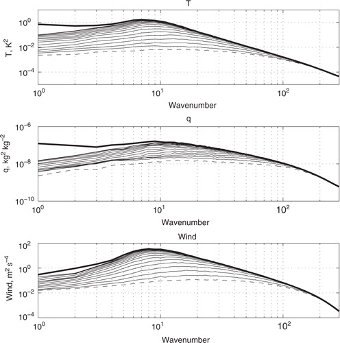
The forecast errors are saturated at the analysis time at wavenumbers higher than 200 (see Errico and Privé, 2013), in that the errors do not increase further with forecast time. At saturation, the error variance would be sum of the variance of the NR fields and the variance of the experimental forecast, assuming that the covariance between the NR and the forecast approaches zero. An estimate of this error variance at saturation is the sum of the variances of the transient fields from the NR and from the day 14 forecast; these estimates are indicated by the heavy lines in Fig. 1. Saturation quickly spreads to all wavenumbers above 100 by day 2 for T and q, and by day 3 for rotational wind. For temperature and moisture, the initial analysis error peaks in the range of wavenumbers 10–20, with a peak closer to wavenumber 20 for wind. The peak error shifts to lower wavenumbers as the forecast progresses, with peak error at day 14 near wavenumber 7 for temperature, wavenumber 10 for q and in the range of wavenumbers 8–10 for wind. By day 14, the error is close to saturation for all fields except at very low wavenumbers, indicating that the covariance between the NR fields and forecast is non-zero. This covariance may be due to the seasonal cycle or large-scale atmospheric patterns with lifespan that is relatively long compared to the sampling period.

As saturation is reached by day 14 for wavenumbers greater than 20, the slope of the error spectra can be calculated and compared with theory. For temperature, the slope of the spectra from wavenumbers 20 to 200 is close to −3, with slope of −3.25 for rotational wind. The slopes in this portion of the spectra for these fields are comparable to other models and agree with observations (Tulloch and Smith, 2006). Specific humidity has a much shallower slope of −1.6 in this wavenumber range, close to $\frac{5}{3}$, indicative of the dominance of mesoscale activity (Gage, 1979). Above wavenumber 200, the spectral slopes increase to near −6.6 for temperature and wind, and −3.4 for specific humidity. This sharp decrease in slope at high wavenumbers is likely due to model damping processes (Augier and Lindborg, 2013) and is in contrast to real-world observations which show a flattening of the slope to approximately $\frac{5}{3}$ at high wavenumbers (Nastrom and Gage, 1985).

Figure 2 shows the ratio of errors at the end of a 24-hour period to the errors at the beginning of the period, a measure of the 24-hour error growth. For purely exponential error growth, the ratio of errors in Fig. 2 would remain constant with time, with ratios greater than one for growing errors and ratios less than one for exponentially decaying errors. For 506 hPa temperature, the peak error growth during the first 24 hours of the forecast occurs near wavenumbers 6–7, then shifts to scales between wavenumbers 10–20 through forecast day 4. After day 4, the magnitude of peak error growth begins to decline as the peak shifts slowly towards lower wavenumbers. The fastest error growth occurs during the first 120 hours of the forecast, with doubling of error variances over a 24-hour period.

Fig. 2 Ratio of spectra of forecast error variances at the beginning and end of a 24-hour period, verified against NR over the July–August period. Each curve represents one forecast time interval at 24-hour intervals from the first 24 hours to the growth between 312 and 336 hours. Top, temperature, K²day⁻¹; centre, 857 hPa specific humidity, kg²kg⁻²day⁻¹; bottom, 356 hPa rotational wind, m²s⁻²day⁻¹.

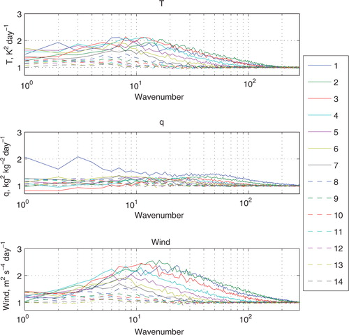
Specific humidity shows a much more complicated growth pattern. The strongest growth is seen during the first 24 hours, with the peak growth at very low wavenumbers. From 24 to 48 hours, the peak error growth shifts to wavenumbers 40–50, with near zero error growth at low wavenumbers. From 48 to 72 hours, there is a decrease in error at wavenumbers less than 5, with peak error growth near wavenumber 30. From day 5 to day 6, the error at low wavenumbers increases, with peak error growth occurring near wavenumber 7, while error growth at high wavenumbers declines. After day 6, there is a more continual decrease of error growth and a shift in peak error growth towards lower wavenumbers. It has been argued (Reynolds et al., 1994; Privé et al., 2013b) that the behaviour of error growth during the first day is a consequence of model error. There is initially large analysis error variance of specific humidity over the tropical oceans. After 24 hours, the error variance begins to decrease over a large region of the tropics, while error variances increase in the extratropics. This pattern implies that the physical processes in the tropics react to imbalances in the analysis and early forecast period, with a timescale of 48–72 hours before the tropical atmosphere recovers.

Upper tropospheric rotational wind error growth follows a simple, classical progression. Initial error growth peaks between wavenumbers 20–25, with error more than doubling in the first 24 hours. Strong error growth continues through day 3, with the peak error growth shifting to lower wavenumbers. After day 3, the peak wavenumber continues to shift towards lower wavenumbers and the magnitude of peak growth steadily declines, nearing saturation by day 12.

3.2. Analysis verification

It is of interest to compare the ‘true’ forecast error verified against the NR with the commonly used metric of forecast error verified against the analysis. These two descriptions of the error will generally differ. Verification against analysis is generally only used for forecasts at 24 hours or longer due to the incestuousness of the comparison at short forecast times. Since the analysis depends on short-term forecasts, covariances between analyses and forecasts at short time ranges can reduce the estimated error variance. At long forecast times where covariances approach zero, differences in the variance of the NR fields and the variance of the GEOS-5 forecast fields will affect the accuracy of the analysis verification method.

Figure 3 shows the ratio of the analysis-verified forecast error variances to the true forecast error variances for days 1 to 5 of the forecast. The 506 hPa temperature error variance calculated by analysis verification is underestimated at 24 hours, but close to the true error variance for large and synoptic scales at the 48-hour forecast and beyond. At high wavenumbers, the analysis verification method significantly overestimates the temperature error variance because the variance of temperature at high wavenumbers is greater for the analysis than for the NR. For 857 hPa specific humidity, the forecast error is severely underestimated at 24 hours, with analysis-verified error variance only 25–50% of the true variance. The analysis-verified error variance still underestimates the true variance for low wavenumbers at 5 days; at this scale, the NR and forecast model have similar variances of humidity, so the underestimation at 120 hours is due to positive covariances between the analyses and forecasts. In contrast to the temperature field, the analysis has lower variance of q at high wavenumbers compared to the NR, resulting in saturation of analysis-verified error variance that is too low at high wavenumbers.

Fig. 3 Ratio of spectra of Control forecast error verified using the analysis to the spectra of forecast error verified using the NR over the July–August period. Heavy solid line, 24-hour forecast; solid thin line, 48-hour forecast; heavy dashed line, 72-hour forecast; thin dashed line, 96-hour forecast; dash-dot line, 120-hour forecast. Top, 506 hPa temperature; centre, 857 hPa specific humidity; bottom, 356 hPa rotational wind component.

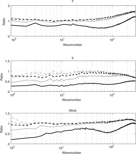
Synoptic and large-scale error variances are significantly underestimated in the analysis-verified error calculation of 300 hPa rotational wind for forecasts of less than 72 hours, with the greatest discrepancy at low wavenumbers. The analysis-verified forecast overestimates error variance at high wavenumbers after the 24-hour forecast period and overestimates the wavenumber one error variance after 96 hours. At long time scales, these overestimations are due to greater error variance at high wavenumbers in the analysis field compared to the NR – there is up to 45% greater variance at high wavenumbers in the analysis and 10% greater variance at very low wavenumbers. This is consistent with the strong damping of high wavenumbers seen in the NR climatology (Errico and Privé, 2013).

The difference between forecast errors verified with respect to analysis or truth profoundly affects error growth estimated by the two verifications. Figure 4 compares the true 24-hour error growth (dashed lines) as a function of wavenumber with the estimated rate of error growth using the analysis field to verify the forecasts (solid lines). The error growth from 24 to 48 hours and the growth from 48 to 72 hours are illustrated for 506 hPa temperature, 857 hPa specific humidity and 300 hPa rotational wind.

Fig. 4 24-hour Control forecast error growth rate spectra over the July–August period. Solid lines indicate verification against analysis; dashed lines indicate verification against NR; heavy lines indicate growth from 24 to 48 hours; and thin lines indicate growth from 48 to 72 hours. Top, 506 hPa temperature K²day⁻¹; centre, 857 hPa specific humidity, kg²kg⁻²day⁻¹; bottom, 356 hPa rotational wind, m²s⁻²day⁻¹.

In all cases, the estimated analysis verification significantly overestimates the magnitude of 24- to 48-hour error growth and also mis-characterises the spectral distribution of error growth. For temperature and humidity, the peak analysis-verified error growth occurs between wavenumbers 50–80, while the actual peak error growth occurs from wavenumbers 8–12 for temperature and wavenumbers 30–50 for q. For rotational wind, the analysis-verified error growth has three peaks, near wavenumbers 2–3, 10–15 and 60–80, while the true error growth has a single peak near wavenumber 10. The largest overestimates of wind error growth occur at very low wavenumbers and from wavenumbers 70–90. The greatest discrepancies in error growth occur at those wavenumbers for which the analysis-verified error estimates (Fig. 3) have the most severe underestimation of true error at the 24-hour forecast time. The magnitude of overestimation is on the order of 200% at peak overestimation for temperature and humidity error growth and 300% overestimation at low wavenumbers for wind error growth.

For the 48- to 72-hour forecast period, the error growth rate estimated by analysis verification is much closer to the true error growth rate, with only a small overestimation for temperature and wind, and somewhat greater overestimation for humidity (approximately 140%). For the 72- to 96-hour forecast period (not shown), the analysis verification method of estimating error growth is very accurate, with overestimation of error growth on the order of 110–120% occurring primarily at wavenumber one.

3.3. Correlations

Correlations between the analysis and verifying forecast fields are commonly used as a measure of forecast skill, such as anomaly correlation. It is of interest to determine if different behaviour is seen for forecast correlations at various spectral scales. Spatial correlations between the temporal anomalies of the forecast and NR fields (labelled C and N, respectively) are calculated for low (1–7), synoptic (8–20) and high (21–287) wavenumber anomalies as follows1 $r=\frac{E\left[\left(C-{\mu }_C\right)\left(N-{\mu }_N\right)\right]}{{\sigma }_C{\sigma }_N}$1

where E is the area and time weighted mean, and µ and σ are, respectively, the areal mean and standard deviations of the Control and NR fields. The correlations for 356 hPa wind and 506 hPa temperature are shown in Fig. 5 as a function of latitude for the progression of the forecast out to 336 hours.

Fig. 5 Correlation of Control forecast fields with NR fields for various spectral ranges for the July–August period. Thick lines indicate analysis, thin solid lines show forecasts at 1 day intervals from 1 to 7 days; thin dashed lines show forecasts from 8 to 14 days. (a,b,c) 506 hPa temperatures; (d,e,f) 356 hPa zonal wind. (a,d) wavenumbers 1–7; (b,e) wavenumbers 8–20; (c,f) wavenumbers 21–287.

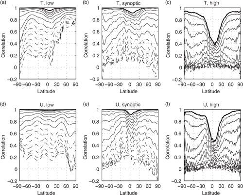
At the analysis time, the lowest correlations are found in the tropics, particularly for high wavenumber anomalies, with correlations near one in the extratropics. The correlations steadily decrease as the forecast progresses. For high wavenumber anomalies, the correlations approach zero by forecast hour 240 for both temperature and wind. After hour 48, a local maximum in correlation between 20S and 30S emerges, while a rapid decline in correlation occurs between 40S and 60S from 48 to 72 hours. The subtropical correlation peak is coincident with the subsidence region of the Hadley circulation, where convection is suppressed. At synoptic scales, the correlations approach zero by hour 336 near the poles, but remain positive between 60S and 60N. As for the high wavenumbers, a peak in correlations develops near 20S, especially for wind, that persists through the first 7 forecast days.

While wind and temperature correlations show similar overall behaviour at high and synoptic wavenumbers, at low wavenumbers the behaviour is quite different for the two fields. For winds, the most rapid decline in correlation occurs in the Northern Hemisphere polar region, with near zero correlation by hour 240, with the slowest decline in correlation near 90S. For temperature, the slowest decline in correlation occurs near 90N, with correlations at hour 336 between 0.7 and 0.8. The fastest decline in correlation occurs near 90S, with correlation near zero at hour 336. The very high correlations in the Northern Hemisphere extratropics (NHEX) for low wavenumbers were unexpected, and may be due to slowly varying large-scale synoptic patterns or seasonal changes. This supports the previous finding of unsaturated error variances at day 14 for low wavenumbers discussed in Section 3.1.

3.4. Growth rates

Prior efforts by Leith (1978), Lorenz (1982), Dalcher and Kalnay (1987), and Simmons and Hollingsworth (2002), among others, have attempted to apply simple functional forms to the growth of forecast errors. The error growth function used by Dalcher and Kalnay (1987) was2 $\frac{dE}{dt}=\gamma +\alpha E-\beta E^2$2

where the change in error variance E with time t includes a linear model error term γ, an exponential growth term αE, and saturation of the error in the extended forecast. In the current study, error growth during the early forecast period is of particular interest in comparison to previous work.

The evolution of the error variances is calculated for the NHEX (30N–60N), SHEX (30S–60S) and tropics (20N–20S). Figure 6 shows the error variance as a function of forecast time for temperature, specific humidity and zonal wind for low (thick line), synoptic (dashed line) and high (thin line) wavenumber bands as previously defined. It is apparent from Fig. 6 that the error growth is often more complicated than the simple functional form of eq. (2).

Fig. 6 Control error variances verified against NR for three regions as a function of forecast time for the July–August period: 60S–30S (SHEX), 20S–20N (Tropics) and 30N–60N (NHEX). Thick line, low wavenumbers 0–7; dashed line, synoptic wavenumbers 8–20; thin solid line, high wavenumbers 21–287. Top row, 506 hPa temperature, K²; centre row, 857 hPa specific humidity, kg²kg⁻²; bottom row, 356 hPa zonal wind, m²s⁻².

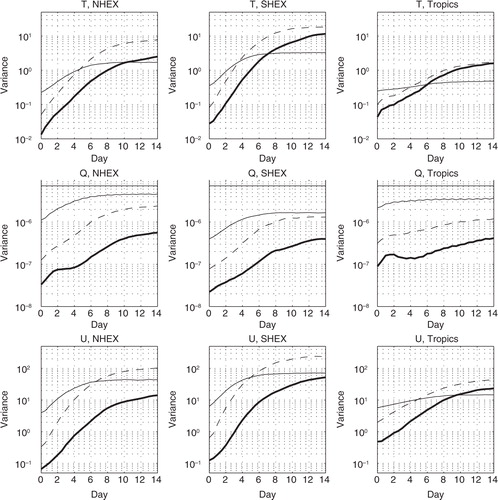
The high wavenumber error growth in the extratropics most closely follows the form of eq. (2), with a period of smooth exponential error growth during the early forecast, followed by saturation after approximately day 7. The high wavenumber error in the tropics has only modest increase between the error variance at the initial time and the saturation error variance. Specific humidity in the tropics has a noticeable diurnal cycle for high wavenumber errors, likely due to the geographic distribution of convection. High wavenumber errors dominate at all forecast times for specific humidity, and during the first few forecast days for temperature and wind in all regions.

Synoptic scale error growth is more complex than high wavenumber error growth, particularly in the tropics. For wind and temperature, the synoptic scale errors appear almost saturated by day 14 and are the dominant error type in the extended forecast. During the early forecast period, the synoptic scale error increases more rapidly than exponential growth for extratropical wind, similar to that seen for high wavenumber error growth. In contrast, in the tropics, temperature and specific humidity have initial rapid error growth during the first day, but slower error growth after 24 hours. Specific humidity in the Southern Hemisphere has exponential error growth during the early forecast, but in the Northern Hemisphere the humidity error growth has similar behaviour to the tropics.

The large-scale error growth is also far from simple. The large-scale errors are not saturated at the end of the 2 weeks forecast. In the Southern Hemisphere extratropics (SHEX), wind and temperature errors exhibit slow error growth during the first day, followed by exponential error growth during the early forecast period and then a gradual deceleration in growth as errors begin to approach saturation. Wind in the NHEX and tropics follows a similar progression of error growth to that in the SHEX. Temperatures in the tropics and NHEX have rapid error growth during the first day, followed by exponential error growth and then a gradual asymptote towards saturation. Specific humidity has an exaggerated pause of growth in the NHEX and tropics, with the tropics actually showing a decline in error variance from day 2 to 4, followed by exponential error growth prior to saturation.

3.5. Perturbation experiment

An additional experiment, designated Perturb, is performed to further investigate error growth during the early forecast period. When generating the synthetic observations, random number generators are used to create the observation error with different seeds used for each observation type and time. In the Perturb case, the seeds used to generate these observation errors are changed, so that the observation errors are different while retaining the statistical properties of the calibrated observations from the Control case. The Perturb case is cycled from 21 June 2011 to 5 September 2011, with 120-hour forecasts launched once daily at 0000 UTC. This case can be considered as a separate realisation of the analysis and forecast cycle in comparison to the Control case.

The Control and Perturb fields can be compared pairwise for forecasts initialised at the same date and time. Direct comparison of the two forecast fields illustrates the growth of initial condition errors in the absence of model error. The variance of the difference between the Control (C) and the Perturb (P) cases can be written as3 $var\left(C-P\right)=var\left(C\right)+var\left(P\right)-2cov\left(C,P\right)$3

where cov is the covariance between C and P. The variance of the difference between the Control and Perturb cases is shown in Fig. 7.

Fig. 7 Variances of differences between Control and Perturb for three regions as a function of forecast time: 60S–30S (SHEX), 20S–20N (Tropics) and 30N–60N (NHEX). Thick line, low wavenumbers 0–7; dashed line, synoptic wavenumbers 8–20; thin solid line, high wavenumbers 21–287. Top row, 506 hPa temperature; centre row, 857 hPa specific humidity, kg²kg⁻²; bottom row, 356 hPa zonal wind.

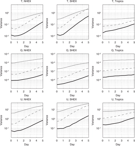
The growth of forecast differences in Fig. 7 is less complex than the growth of forecast errors, with behaviour closer to the simplified form described by eq. (2). This implies that model error may be the source of some of the complex growth patterns seen in Fig. 6. There are some interesting features in the difference growth behaviour, particularly in the initial forecast period, where the variance of forecast differences sometimes shows a slight dip in growth during the first day of the forecast, most notably for large-scale differences of temperature in the extratropics. This dip could have several possible causes, including an initial decrease in the variance of the fields in either case, or by the fields in the two cases initially becoming more alike.

The variances and covariances of the Control and Perturb fields are shown in Fig. 8. A wide variety of behaviours are seen, including increasing, decreasing and constant variances with forecast time. There is no consistent behaviour that would suggest that the initial dip in forecast difference variances is caused by decreases in both or either corresponding forecast field variances.

Fig. 8 Variance of Control fields (thick solid line), variance of Perturb fields (thin line) and covariance of Control and Perturb fields (dashed line) for the July–August period: 60S–30S (SHEX), 20S–20N (Tropics) and 30N–60N (NHEX) for low wavenumbers. Top row, 506 hPa temperature, K²; centre row, 857 hPa specific humidity, kg²kg⁻²; bottom row, 356 hPa zonal wind, m²s⁻².

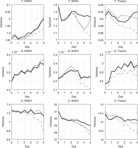
The variances of the Control and Perturb cases show similar but not identical behaviour. Corresponding values differ from each other by only a few percent in most cases (note scale of the ordinate in Fig. 8). In the northern hemisphere, the variances of temperature and humidity notably increase throughout the forecast period, along with the covariance of the Control and Perturb fields. This is believed to be due to seasonal increases in the variances of temperature and humidity during the month of August. Covariances also tend to increase when total variance increases, but note that there is greater separation of the covariance from the variances as the forecast progresses.

Since comparison of the Control and Perturb experiments excludes model error, while the actual error of both cases incorporates a significant amount of such error, short-term error growth is grossly under-estimated by variances of differences of the Perturb and Control fields, with some fields in some locations showing instead error decay. Initial perturbations can be constructed such that such decay is not observed, such as by using singular vectors (Farrell, 1988; Buizza et al., 1993; Palmer et al., 1998), but in this example this would just mask the real cause of error growth, namely model error, and therefore likely misrepresent some characteristics of the latter. In this pair of experiments, a large portion of the initial perturbations apparently project onto non-growing or even decaying short-term singular vectors, which is unsurprising given what is known of the spectra of such singular vectors (Errico et al., 2001) and the projections of analysis error on them (Leutbecher and Lang, 2014).

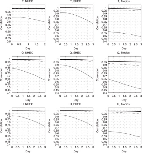
The correlation of the Control and Perturb fields (Fig. 9) features a very slight increase in correlations from the analysis state to the 12-hour forecast for all scales of NHEX temperatures and large and synoptic scales of SHEX temperatures, indicating that the fields become more alike during the very early forecast period – these are the forecast difference fields that showed a pronounced dip in the early forecast. However, other variables exhibit monotonically decreasing correlations during the early forecast period.

Fig. 9 Correlations between Control and Perturb forecast fields for three regions as a function of forecast time for the July–August period: 60S–30S (SHEX), 20S–20N (Tropics) and 30N–60N (NHEX). Thick line, low wavenumbers 0–7; dashed line, synoptic wavenumbers 8–20; thin solid line, high wavenumbers 21–287. Top row, 506 hPa temperature; centre row, 857 hPa specific humidity; bottom row, 356 hPa zonal wind.

The behaviour of the forecast differences is further explored by calculating the correlation of the error fields. The forecast errors verified against the NR, N, are defined as4 $\tilde{C}=C-N$4 5 $\tilde{P}=P-N$5

Then, the covariance of the forecast errors may be written as6 $cov(\tilde{C},\tilde{P})=cov(C,P)+var(N)-cov(C,N)-cov(P,N)$6

The correlation r between the errors of the two realisations is likewise7 $r\left(\tilde{C},\tilde{P}\right)=\frac{cov\left(\tilde{C},\tilde{P}\right)}{\sqrt{var\left(\tilde{C}\right)}\sqrt{var\left(\tilde{P}\right)}}$7 8 $r\left(\tilde{C},\tilde{P}\right)=\frac{cov\left(C,P\right)+var\left(N\right)-cov\left(C,N\right)+cov\left(P,N\right)}{\sqrt{var\left(\tilde{C}\right)}\sqrt{var\left(\tilde{P}\right)}}$8

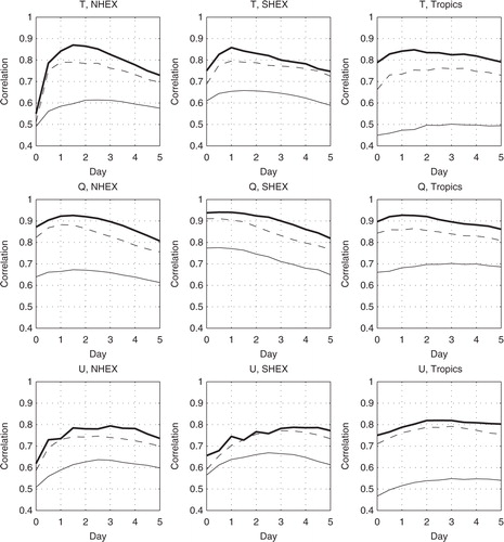
As seen in Fig. 10, the greatest increases in $r(\tilde{C},\tilde{P})$ occur during the first day of the forecast; these correlations continue to increase for up to 3 days, after which they begin to decrease. The weakest and earliest peak in correlation is seen for humidity in the SHEX region, with the latest peak correlations occurring for wind, and the most exaggerated peak seen for temperature in the NHEX region. It is notable that the increase in forecast error correlations occurs not just for larger scales, but also for the high wavenumber errors. This pronounced increase in error correlations, not seen in the correlation of the fields in Fig. 9, indicates that the difference between the forecasts and the NR grows much more quickly than the differences between the paired experimental forecasts.

Fig. 10 Correlations between Control forecast errors and Perturb forecast errors for three regions as a function of forecast time for the July–August period: 60S–30S (SHEX), 20S–20N (Tropics) and 30N–60N (NHEX). Thick line, low wavenumbers 0–7; dashed line, synoptic wavenumbers 8–20; thin solid line, high wavenumbers 21–287. Top row, 506 hPa temperature; centre row, 857 hPa specific humidity; bottom row, 356 hPa zonal wind.

As the forecast time t _F increases, cov(C,P), cov(C,N), cov(P,N) are all expected to decrease and approach zero. var(N) may be approximated as constant as t _F increases, and var(C)≈var(P). Thus,9 $\underset{t_F\to \infty }{lim}cov\left(\tilde{C},\tilde{P}\right)=var\left(N\right)$9 10 $\underset{t_F\to \infty }{lim}r\left(\tilde{C},\tilde{P}\right)=\frac{var\left(N\right)}{\sqrt{var\left(\tilde{C}\right)}\sqrt{var\left(\tilde{P}\right)}}$10

If the variance of the free-running forecast model is similar to the variance of the NR, then11 $\underset{t_F\to \infty }{lim}var\left(C\right)=var\left(N\right)$11 12 $\underset{t_F\to \infty }{lim}var\left(\tilde{C}\right)=2var\left(N\right)$12 13 $\underset{t_F\to \infty }{lim}r\left(\tilde{C},\tilde{P}\right)=\frac{var\left(N\right)}{2var\left(N\right)}=\frac{1}{2}$13

The only correlations that appear to asymptote prior to 120 hours are the high wavenumber correlations in the tropics, although a forecast longer than 14 days may be needed to determine the ultimate correlation. The correlation of tropical temperature and winds for high wavenumbers asymptote to values close to 0.5, while specific humidity correlations asymptote to a value near 0.7. The NR has greater variances of specific humidity compared to the experimental forecasts for wavenumbers higher than 10, while the NR has smaller variances of temperature compared to experimental forecasts for wavenumbers higher than 20.

4. Discussion

Although previously published error spectra have most frequently been calculated for geopotential height or kinetic energy, a comparison between prior studies can be made with the current results. For wind and temperature, mesoscale and smaller scale errors initially dominate, but after 3–6 days, synoptic scale errors become prominent. High wavenumber errors remain dominant for specific humidity throughout the extended forecast, likely due to processes such as small-scale convective processes in the tropics and the generation of filaments of moisture by midlatitude synoptic systems. Boer (2003) calculated the mean and transient error spectra of 500 hPa geopotential height for the CMC operational Global Environmental Multiscale model and found a progression of error spectra for the first six forecast days that is qualitatively similar to the error spectra in Fig. 1, including rapid saturation at high wavenumbers and a shift of spectral peak towards lower wavenumbers as the forecasts progress.

The slope of the saturated error spectra of wind and temperature in the mid and upper troposphere from wavenumbers 20 to 200 is approximately −3 as shown in Section 3.1, indicative of quasi-geostrophic two-dimensional turbulence (Charney, 1971). The slopes of the power spectra of errors are expected to be equal to the slopes of the full fields once the errors have saturated. Observations of wind and temperature (Nastrom and Gage, 1985) demonstrate a transition from a spectral slope of −3 at lower wavenumbers to −5/3 at higher wavenumbers. This transition is not seen here, as the spectral slope becomes increasingly negative at very high wavenumbers due to model damping. On the other hand, the spectra of specific humidity has a slope of −5/3 over wavenumbers 20–200 before transitioning to a steeper slope at very high wavenumbers, possibly indicating the dominance of mesoscale activity.

The growth rate of forecast errors has been the subject of numerous studies, as described in Section 3.4. The classic portrayal of error growth is one of exponential growth during the early forecast period with a gradual asymptote towards a saturation value at the extended forecast (Leith, 1978). This behaviour is most clearly seen in these results for high wavenumber forecast errors, but more complicated error growth is observed for low and synoptic wavenumber errors, particularly in the tropics and for specific humidity, where rapid error growth during the first 48 hours is followed by a period of much weaker error growth (or even a decrease in error variance). The initial surge in error variance of temperature and humidity in some regions may be due to physical processes in the model that react to imbalances in the initial state or to an analysis field that differs significantly from the preferred climatology of the model (Reynolds et al., 1994). This surge is strongest in the tropics and summer hemisphere, where convection plays a stronger role than in the winter extratropics. The initial slow growth of wind error globally, as well as Southern Hemisphere temperature error growth, may be due to the dampening of those initial condition errors that project onto decaying modes.

In practice, some form of self-verification is often used to calculate forecast error, generally by using the analysis field as the ‘truth’. In the OSSE framework, the existence of the NR allows the explicit calculation of analysis and forecast error, and these different methods of verification have been compared in Section 3.2. Overall, self-verification using the analysis field as truth significantly underestimates the true forecast errors during the early forecast period. For wind, the analysis-verified forecast errors approach the true errors after 48 hours, with the temperature analysis-verified forecast error rapidly approaching the true magnitudes by 48 hours. Specific humidity analysis-verified errors are slower to improve, with some underestimation remaining at 120 hours. At high wavenumbers, differences in the climatologies of field variances dominate the discrepancies in analysis-verified errors after the 24-hour forecast. Because of this considerable underestimation by analysis-verified error, the early forecast period growth rates are significantly overestimated. These findings indicate that caution is warranted when analysis-verification is used to quantify errors during the early forecast period.

One aspect of the analysis-verified errors worth noting is that the discrepancy in the wind error growth during the early forecast period was greatest at large scales, while temperature and humidity have the greatest discrepancy in error growth at high wavenumbers. Presently, no explanation of this result is offered.

The correlations between the forecast and NR fields decrease monotonically with forecast time, as expected. The weakest initial correlations occur for small-scale features, particularly in the tropics where convective processes dominate at these scales. Correlations of high wavenumber anomalies decline quickly, reaching near zero values by the latter period of the extended forecast, corresponding to the saturation of errors at these wavenumbers.

The correlations of analysis and forecast errors between the Control and Perturb cases exhibit different behaviour than the correlations of the actual Control and Perturb fields. There is generally an initial increase in correlation of the two error fields before the correlations begin to decline into the medium-range forecast. This indicates that during the initial period, error grows preferentially in certain locations, with the same sign in both forecasts, or conversely, random, uncorrelated errors that differ between the two experiments may be damped. After this initial period, the two forecasts have diverged sufficiently that preferential error growth no longer occurs in the same regions and/or differs in sign, and the correlation between error field declines. Peak error correlations occur earlier in the forecast for temperature and specific humidity, with peaks at 1–2 days, compared with peak at 2–4 days for wind. However, aside from temperature in the extratropics, the correlations of the full fields of the two experiments do not increase in the early forecast period. This implies that the NR fields diverge from the experimental forecasts much more rapidly than the paired forecasts diverge from each other.

The results of these experiments are generally in agreement with prior studies (e.g. Boer, 1994, 2003; Reynolds et al., 1994; Simmons and Hollingsworth, 2002), particularly for the medium to extended forecast range. Model error is found to have a significant impact on the early forecast period, resulting in error growth that does not follow the theoretical framework laid out by Leith (1978), Dalcher and Kalnay (1987), and others. The accuracy of self-analysis verification for estimating forecast errors is significantly impacted by the incestuousness of the comparison for the first 2 to 3 days of the forecast.

The primary caveat with OSSE studies is applicability of the experiments to the real world, since the OSSE context is a simulation. The results are best considered qualitatively rather than quantitatively. There are known deficiencies of certain aspects of the OSSE; for example, the NR does not have realistic variance at high wavenumbers, presumably due to unrealistic damping. Thus, error variances for wavenumbers above 100 do not display realistic behaviours in the OSSE. Also, forecast skills in the OSSE have been found to be somewhat higher than real forecasts, implying that model error may be insufficient in the OSSE and that forecast errors in the real world have greater magnitude.

Acknowledgements

The ECMWF Nature Run was provided by Erik Andersson through arrangements made by Michiko Masutani. Support for this project was encouraged by Steven Pawson and provided by GMAO core funding.

References

- Andersson E. , Fisher M. , Munro R. , McNally A . Diagnosis of background errors for radiances and other observable quantities in a variational data assimilation scheme, and the explanation of a case of poor convergence. Q. J. Roy. Meteorol. Soc. 2000; 126: 1455–1472.
- Augier P. , Lindborg E . A new formulation of the spectral energy budget of the atmosphere, with application to two high-resolution general circulation models. J. Atmos. Sci. 2013; 70: 2293–2308.
- Baer F . An alternate scale representation of atmospheric energy spectra. J. Atmos. Sci. 1972; 29: 649–664.
- Boer G . Predictability regimes in atmospheric flow. Mon. Weather Rev. 1994; 122: 2285–2295.
- Boer G . Predictability as a function of scale. Atmos. Ocean. 2003; 41: 203–215.
- Buizza R. , Tribbia J. , Molteni F. , Palmer T. N . Computation of optimal unstable structures for a numerical weather prediction model. Tellus A. 1993; 45: 388–407.
- Charney J . Geostrophic turbulence. J. Atmos. Sci. 1971; 28: 1087–1095.
- Charney J. , Fleagle R. , Riehl H. , Lally V. , Wark D . The feasibility of a global observation and analysis experiment. Bull. Am. Meteorol. Soc. 1966; 47: 200–220.
- Dalcher A. , Kalnay E . Error growth and predictability in operational ECMWF forecasts. Tellus A. 1987; 39: 474–491.
- Errico R. , Ehrendorfer M. , Raeder K . The spectra of singular values in a regional model. Tellus A. 2001; 53: 317–332.
- Errico R. , Privé N . An estimate of some analysis error statistics using the GMAO observing system simulation framework. Q. J. Roy. Meteorol. Soc. 2013; 130: 1005–1012.
- Errico R. M. , Yang R. , Privé N. , Tai K.-S. , Todling R. , co-authors . Validation of version one of the Observing System Simulation Experiments at the Global Modeling and Assimilation Office. Q. J. Roy. Meteorol. Soc. 2013; 139: 1162–1178.
- Farrell B . Optimal excitation of neutral Rossby waves. J. Atmos. Sci. 1988; 45: 163–172.
- Gage K . Evidence for a k −5/3 law inertial range in mesoscale two-dimensional turbulence. J. Atmos. Sci. 1979; 36: 1950–1954.
- Han Y. , van Delst P. , Liu Q. , Weng F. , Yan B. , co-authors . 2006. JCSDA Community Radiative Transfer Model (CRTM) – Version 1. NOAA Tech. Rep., NESDIS 122, 40 pp.
- Hollingsworth A. , Lonnberg P . The statistical structure of short-range forecast errors as determined from radiosonde data. Part 1: the wind-field. Tellus A. 1986; 38: 111–136.
- Kleist D. , Parrish D. , Derber J. , Treadon R. , Wu W.-S. , co-authors . Introduction of the GSI into the NCEP global data assimilation system. Weather Forecast. 2009; 24: 1691–1705.
- Leith C . Theoretical skill of Monte Carlo forecasts. Mon. Weather Rev. 1974; 102: 409–418.
- Leith C . Objective methods for weather prediction. Ann. Rev. Fluid Mech. 1978; 10: 107–128.
- Leith C. , Kraichnan R . Predictability of turbulent flows. J. Atmos. Sci. 1972; 29: 1041–1058.
- Leutbecher M. , Lang S . On the reliability of ensemble variance in subspaces defined by singular vectors. Q. J. Roy. Meteorol. Soc. 2014; 140: 1453–1466.
- Lorenz E . Deterministic nonperiodic flow. J. Atmos. Sci. 1963; 20: 130–141.
- Lorenz E . Atmospheric predictability experiments with a large numerical model. Tellus. 1982; 34: 505–513.
- Lorenz E . The Essence of Chaos.
- McCarty W. , Errico R. , Gelaro R . Cloud coverage in the joint OSSE nature run. Mon. Weather Rev. 2012; 140: 1863–1871.
- Nastrom G. , Gage K . A climatology of atmospheric wavenumber spectra of wind and temperature observed by commercial aircraft. J. Atmos. Sci. 1985; 42: 950–960.
- Orrell D. , Smith L. , Barkmeijer J. , Palmer T . Model error in weather forecasting. Nonlinear Process. Geophys. 2001; 8: 357–371.
- Palmer T. , Gelaro R. , Barkmeijer J. , Buizza R . Singular vectors, metrics, and adaptive observations. J. Atmos. Sci. 1998; 55: 633–653.
- Palmer T. , Hagedom R . Predictability of Weather and Climate.
- Privé N. , Errico R. , Tai K.-S . The role of model and initial condition error in numerical weather forecasting investigated with an observing system simulation experiment. Tellus A. 2013b; 65: 21740.
- Privé N. , Errico R. , Tai K.-S . Validation of forecast skill of the Global Modeling and Assimilation Office observing system simulation experiment. Q. J. Roy. Meteorol. Soc. 2013c; 139: 1354–1363.
- Reale O. , Terry J. , Masutani M. , Andersson E. , Riishojgaard L. , co-authors . Preliminary evaluation of the European Centre for Medium-range Weather Forecasts (ECMWF) nature run over the tropical Atlantic and African monsoon region. Geophys. Res. Lett. 2007; 34: L22810.
- Reynolds A. , Webster P. J. , Kalnay E . Random error growth in NMC's global forecasts. Mon. Weather Rev. 1994; 122: 1281–1305.
- Rienecker M. , Suarez M. , Todling R. , Bacmeister J. , Takacs L. , co-authors . The GEOS-5 Data Assimilation System – Documentation of Versions 5.0.1, 5.1.0 and 5.2.0. . 2008. Technical Report 27, NASA Tech. Memo., NASA/TM–2008–104606, vol. 27, 118 pp.
- Savijärvi H . Error growth in a large numerical forecast system. Mon. Weather Rev. 1995; 123: 212–221.
- Simmons A. , Hollingsworth A . Some aspects of the improvement in skill of numerical weather prediction. Q. J. Roy. Meteorol. Soc. 2002; 128: 647–677.
- Simmons A. , Mureau R. , Petroliagis T . Error growth and predictability estimates for the ECMWF forecasting system. Q. J. Roy. Meteorol. Soc. 1995; 121: 1739–1771.
- Smagorinsky J . Problems and promises of deterministic extended range forecasting. Bull. Am. Meteorol. Soc. 1969; 50: 286–311.
- Swartzrauber P. , Spotz W . Generalized discrete spherical harmonic transforms. J. Comput. Phys. 2000; 159: 212–230.
- Thompson P . Uncertainty of initial state as a factor in the predictability of large scale atmospheric flow patterns. Tellus. 1957; 9: 275–295.
- Tribbia J. , Baumhefner D . Scale interactions and atmospheric predictability: an updated perspective. Mon. Weather Rev. 2004; 132: 703–713.
- Tulloch R. , Smith K . A theory for the atmospheric energy spectrum: depth limited temperature anomalies at the tropopause. Proc. Natl. Acad. Sci. USA. 2006; 103: 14690–14694.