Thermal air–sea coupling in hindcast simulations for the North Sea and Baltic Sea on the NW European shelf

Abstract

This article compares interactively coupled atmosphere–ocean hindcast simulations with stand-alone runs of the atmosphere and ocean models using the recently developed regional ocean–atmosphere model NEMO-Nordic for the North Sea and Baltic Sea. In the interactively coupled run, the ocean and the atmosphere components were allowed to exchange mass, momentum and heat every 3 h. Our results show that interactive coupling significantly improves simulated winter sea surface temperatures (SSTs) in the Baltic Sea. The ocean and atmosphere stand-alone runs, respectively, resulted in too low sea surface and air temperatures over the Baltic Sea. These two runs suffer from too cold prescribed ERA40 SSTs, which lower air temperatures and weaken winds in the atmosphere only run. In the ocean-only run, the weaker winds additionally lower the vertical mixing thereby lowering the upward transport of warmer subpycnocline waters. By contrast, in the interactively coupled run, the ocean–atmosphere heat exchange evolved freely and demonstrated good skills in reproducing observed surface temperatures. Despite the strong impact on oceanic and atmospheric variables in the coupling area, no far reaching influence on atmospheric variables over land can be identified. In perturbation experiments, the different dynamics of the two coupling techniques is investigated in more detail by implementing strong positive winter temperature anomalies in the ocean model. Here, interactive coupling results in a substantially higher preservation of heat anomalies because the atmosphere also warmed which damped the ocean to atmosphere heat transfer. In the passively coupled set-up, this atmospheric feedback is missing, which resulted in an unrealistically high oceanic heat loss. The main added value of interactive air–sea coupling is twofold: (1) the elimination of any boundary condition at the air–sea interface and (2) the more realistic dynamical response to perturbations in the ocean–atmosphere heat balance, which will be essential in climate warming scenarios.

• air–sea interaction
• dynamical downscaling
• climate modelling

1. Introduction

Interactive air – sea coupling is applied more and more in regional high-resolution modelling. Stand-alone models for the ocean and atmosphere have been widely used in regional simulations of the present day climate (e.g. Jacob et al., 2001; Janssen et al., 2001; Schrum, 2001; Lehmann et al., 2002; Meier and Kauker, 2003; Weisse et al., 2009; Feser et al., 2011; Löptien and Meier, 2011; Mathis et al., 2013; Su et al., 2014). Those models are driven by either prescribed boundary fields or fluxes usually obtained from re-analysis data. In such a rigid set-up, the prescribed boundary does not respond to any changes in the modelled parameters (e.g. temperature) with the exception that the modelled SST sometimes is used to calculate, for example, sensible heat and long-wave fluxes instead of prescribing them, which then introduces an additional feedback. However, the dynamical response of the changing atmospheric boundary is still missing. Nevertheless, any re-analysis data at the boundaries will prevent the model from drifting too far from observations. In quasi-equilibrium simulations for the present day period, this coupling technique works fine to reproduce observed patterns of oceanic parameters on the regional scale. However, when driven by global climate model output as is the case in downscaling simulations of climate warming scenarios, the close relationship to the forcing GCM may be problematic. This is because a large part of the response to anthropogenically forced climate warming is determined by interacting feedback loops between the ocean and the atmosphere, which influence the heat distribution between the ocean and the atmosphere (e.g. Watanabe and Kimoto, 2006).

However, in stand-alone models such feedbacks are represented only insufficiently because, for example, any temperature change at the sea surface is not communicated to the atmosphere and thus, the ocean lacks an important response from the atmosphere. Therefore, in today's state-of-the-art global climate models the oceanic and atmospheric model compartments are coupled interactively such as simulations carried out in the frame of the Coupled Model Intercomparison Project (CMIP) under the umbrella of the World Climate Research Programme (WCRP). Thus, any change in the lower/upper boundary conditions in the one model component is communicated interactively during the simulation to the upper/lower boundary field of the other component.

In contrast to global climate models that are used to simulate the complex interactions of climate processes and their change on the long term, most regional models are usually developed to reproduce the mean state-of-the present-day climate rather than to predict the potential impact of climate change (e.g. Kerr, 2013). This might make their application for projecting the climate change problematic due to following three reasons. (1) For many regions, the climate change is expected to be significantly larger than the internal variability seen in near equilibrium simulations for the present climate (Christensen et al., 2007) to which regional models have been tuned to. (2) A further challenge for regional models is related to the transient behaviour of climate change. Due to the different internal time scales of the ocean and the atmosphere, it is difficult to assess from uncoupled models, how fast the coupled ocean–atmosphere system will reach a new equilibrium. (3) Finally, in future scenarios, regional models have to be driven by the output of climate models, which nowadays are mostly interactively coupled. Hence, any climate change signal penetrates from a (global) model where atmospheric variability is modulated by the coupled ocean–atmosphere system into a (regional) model that assumes the stochastic atmospheric variability to be independent from internal ocean modes. These reasons promote the idea of applying the interactively coupling technique also in regional models.

Regions of intense ocean–atmosphere coupling, that is, areas where such feedbacks become important, are the tropics and the high latitudes (e.g. Fedorov, 2008). In these regions, the use of coupled models versus uncoupled models impacts mainly on the variability of surface hydrographic properties. In the tropics, the thermal ocean–atmosphere coupling is essential (Latif et al., 2001; Sun et al., 2006) with regard to the El Nino Southern Oscillation (e.g. Sun et al., 2006; Brown et al., 2011) and the Madden Julian Oscillation (Zhang, 2005). Kwon et al. (2010) found a northward displacement of the intertropical convergence zone by interactively coupling a mixed layer ocean model to an atmospheric GCM.

In the temperate mid-latitudes, the ocean–atmosphere coupling is largely controlled by stochastic atmospheric variability (e.g. Hasselmann, 1976; Bhatt et al., 1998). Here, a rather passive ocean response induces spectral energy particularly at lower frequencies and presumably enhances the decadal variability, which might be larger than the climate change signal in the near future (e.g. Matei et al., 2012). The first-order effect of interactive thermal air–sea coupling at mid-latitudes is an enhanced variance of both SSTs and air temperatures. This is because in interactively coupled models both the ocean and atmosphere temperatures can adapt to each other, which reduces the air–sea heat fluxes and enhances temperature variability that has been described as reduced thermal damping (e.g. Barsugli and Battisti, 1998; Fedorov et al., 2008; Sura and Newman, 2008). In the North Atlantic, this effect of enhanced SST variability is well documented (e.g. Manabe and Stouffer, 1996; Bhatt et al., 1998; Watanabe and Kimoto, 2006), and the stability of the Atlantic Meridional Overturn Circulation has been found to be unrealistically instable in uncoupled ocean models when SSTs are relaxed too tightly to the surface boundary conditions (e.g. Mikolajewicz and Maier-Reimer, 1994).

In contrast to the aforementioned work which investigated air–sea coupling affecting mostly in the open ocean, our study area is located in the NW European shelf and thus lacks the inert and slow responding deep ocean. Thus, it is questionable how far these results can be transferred to the North Sea and Baltic Sea, which have by far lower heat content and, therefore, might be expected to be coupled much more tightly to the atmosphere than this is the case for the open ocean. Early work by Marotzke and Pierce (1997) and Nilsson (2000) using conceptual energy balance models including a slab mixed layer ocean could clearly distinguish different time scales for the damping of SST anomalies due to air–sea heat exchange and lateral advection. Large-scale SST anomalies were found to behave rather diffusively in the atmosphere. Nilsson (2000) also emphasised the importance of local bulk formulae for the damping of small-scale temperature anomalies.

In the North Sea and Baltic Sea, the thermal air–sea coupling is strongly controlled by the seasonal cycle of the air–sea temperature difference, which changes its sign twice a year. In addition to that, the winds and storm activity largely impacts on the mixed layer depth. The mixed layer thickness in turn controls how fast the ocean will adapt to changes in the atmosphere and how fast a new equilibrium is reached.

In the last decades, interactive air–sea coupling has also been applied in high-resolution regional models (see Seo et al., 2007 and Omstedt et al., 2014 for a comprehensive summary) especially for the North Sea and Baltic Sea shelf region (Gustafsson et al., 1998; Hagedorn et al., 2000; Döscher et al., 2002; Schrum et al., 2003, Döscher and Meier, 2004; Lehmann et al., 2004; Tian et al., 2013). Gustafsson et al. (1998) coupled the weather forecast model HIRLAM to an ocean GCM and found an improvement of simulated summer SSTs. However, the authors had to apply data assimilation techniques to prevent the model drifting towards a less realistic mean state. Lehmann et al. (2004) applied the coupled ocean – atmosphere model BALTIMOS on the simulation of extreme inflow events in the Baltic Sea. Tian et al. (2013) found only slight differences in simulated 2 m air temperatures and SSTs between the interactively and passively coupled model simulations for coastal regions of the Baltic Sea. Hagedorn et al. (2000) obtained realistic results at least during summer by coupling the regional atmosphere model REMO to the Kiel 3-D ocean GCM. Döscher et al. (2002) presented the coupled ocean – atmosphere model RCAO and obtained realistic results for the Baltic Sea without any drift in a 5-yr simulation. Sein et al. (2015) presented the regional coupled model REMO/MPIOM and showed improvements for the North Atlantic and the North Sea hydrography compared to globally coupled models.

Schrum et al. (2003) were the first to apply a fully coupled high-resolution ocean–atmosphere GCM covering both the North Sea, and Baltic Sea in a simulation of a full seasonal cycle. The authors found the SST (and connected sea ice) to be very sensitive to the coupling technique. However, owing to the short simulation period of only 1 yr, it is not clear if the described interactive coupling effects result also in different climatological mean state on longer multidecadal time scales. Moreover, compared to the non-interactive passive coupling the introduction of interactive ocean–atmosphere coupling will increase the degree of freedom in the coupled system. In turn, this must be expected to feed back somehow on the model performance. Thus, long-term simulations are necessary for the fully coupled model system to assess the question if such a coupled model can appropriately be applied in longer term simulations for the North Sea/Baltic Sea region.

As a first step to answer the aforementioned questions, we here present the newly developed interactively coupled ocean-atmosphere GCM RCA4/NEMO (hereafter referred to as NEMO-Nordic) applied on 48-yr hindcast simulations. We use this model to assess the interactive coupling impacts on the mean present-day climatology in the North Sea/Baltic Sea, and how the dynamic behaviour is influenced by the coupling. Apart from whether the ocean and atmosphere components are coupled interactively or passively, it is important how air–sea fluxes are calculated. In our interactive model, fluxes are exchanged while in the stand-alone version bulk formulae were used. This may also lead to differences in the performance of the models.

2. Experimental set-up

The model used for this study is the regional coupled ocean–atmosphere NEMO-Nordic GCM. The ocean component is based on the Nucleus for European Modelling of the Ocean (NEMO, Madec, 2011) – a model, which was set up for the North Sea and Baltic Sea (Hordoir et al., 2013; Fig. 1). The horizontal grid distance is 3.7 km in W–E direction and varies between 4.0 and 2.5 km in S–N direction. The water column is divided into 56 unevenly placed vertical z-levels. The uppermost level is 3-m thick and has a free surface. Furthermore, the vertical discretisation is modified by an additional term, which scales the model layers according to the variations of column thickness due to sea-surface undulations [see NEMO reference manual, Madec (2011)]. Vertical mixing follows the k–ɛ turbulence closure of Madec (2011). Adaptions for the specific conditions in the North Sea and Baltic Sea with regard to vertical mixing have been made. To capture the strong tidal influence in the southern North Sea and the English Channel, the tidal dynamics is included following Egbert et al. (2010) and Egbert and Erofeeva (2002). River runoff was prescribed from the hydrology model E-HYPE (Donnelly et al., 2013, 2015). The model includes the dynamic thermodynamic sea ice model LIM3 (Vancoppenolle et al., 2009).

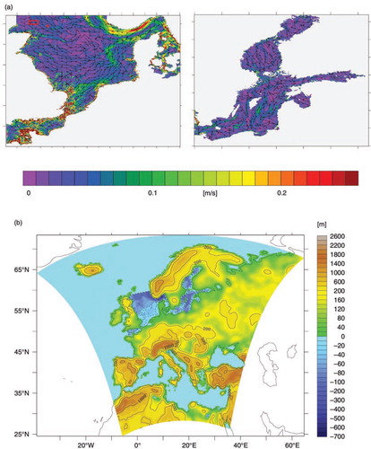
Fig. 1 (a) Model domain and annual mean surface circulation of the NEMO-Nordic OGCM. The red box indicates the region of temperature local anomaly perturbation in experiment (Section 4.1). The red cross indicates the station where time series have been sampled (0.5°W; 57.9°N). (b) Model domain of the regional atmospheric model RCA4. Bathymetry has been taken from the NEMO-Nordic ocean model. Contour lines are −50, −30, 200, 500 and 1000 m.

The NEMO model is coupled to the Rossby Centre regional Atmospheric climate model RCA4 (Kupiainen et al., 2014; Wang et al., 2015). The hydrostatic model RCA4 is set up with a horizontal resolution of about 24 km. The model domain comprises Europe, northern Africa and covers parts of the adjacent Northeast Atlantic, and the Mediterranean Sea, and the Black Sea (Fig. 1b). The mass and energy exchanges between NEMO and RCA4 are done by the OASIS3 coupler (Valcke et al., 2003). A detailed description and validation of prognostic variables against observations is given in Samuelsson et al. (2011) and Dieterich et al. (2013).

Since we investigate here the specific impact of interactive coupling on the thermal state of the ocean, we do not provide a comprehensive validation of the main prognostic ocean variables. This can be found, along with a comprehensive technical model description, in Wang et al. (2015). However, for assessing the validity of the specific results presented here, we use the observed temperature climatology of the Bundesamt für Seeschifffahrt und Hydrographie (BSH), Hamburg/Germany. For the North Sea, the BSH produces weekly composite SST analyses of in situ measurements using objective statistical interpolation methods on a 20-km Lambert equal area grid. In data sparse regions, the analysis employs a blending algorithm for Advanced Very High Resolution Radiometer SSTs. The provided monthly mean data were computed from the weekly SST analysis. In the Baltic Sea, only satellite derived data are processed. This procedure yields a high-quality data set with sufficient spatial coverage to serve as a validation reference in this study.

In this study, we basically compare two different model set-ups. In one set-up, the ocean model NEMO and the atmospheric model RCA4 were allowed to directly exchange mass, energy and momentum fluxes (as indicated in Fig. 2) online during the simulation in the RCA4-NEMO model with a coupling frequency of 3 h [hereafter interactively coupled ocean and atmosphere (ICO and ICA) simulations, Table 1]. In the passively coupled case, the oceanic model component NEMO was driven by prescribed atmospheric boundary conditions [experiment 2b in Fig. 2, hereafter referred as passively coupled ocean (PCO) and passively coupled atmosphere (PCA) simulations, Table 1]. The prescribed forcing fields are indicated in Fig. 2 and were taken from a downscaled ERA40 hindcast simulation using the regional atmospheric model RCA4 (2a in Fig. 2 hereafter referred as PCA simulation).

Fig. 2 Experimental set-up and exchange variables between the ocean and atmosphere model components. ICA=interactively coupled atmosphere, ICO=interactively coupled ocean, PCA=passively coupled atmosphere, PCO=passively coupled ocean.

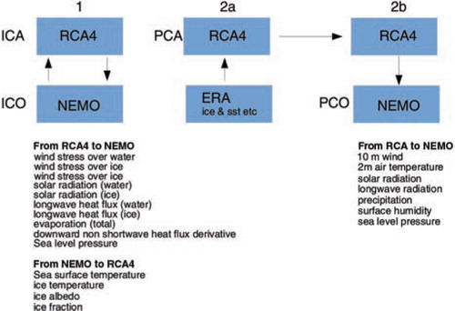
Table 1 Model simulations

Interactively coupled	Domain	Model	Period
ICO	Ocean	NEMO	1961–2009
ICA	Atmosphere	RCA4	1961–2009
Passively coupled
PCO	Ocean	NEMO	1961–2009
PCA	Atmosphere	RCA4	1961–2009
Perturbation experiments			Period
Local anomaly	12°C	<50 m	1.1–31.12 1990^a
Basinwide anomaly	+5°K	<50 m	1.1–31.12 1990^a
Lateral anomaly	+5°K		1990–1994^a

^aThe perturbation experiments were carried out for both the interactively coupled and the passively coupled set-ups.

The lateral boundary conditions are the same for the two set-ups. The open boundaries for NEMO are taken from an observed climatology (Janssen et al., 1999). The atmospheric regional model RCA4 is driven by ERA40 re-analysis data. The coupling impact on the ocean is the main focus here. A comparison of the two RCA4 outputs gives insight into the coupling impact on the atmosphere.

The experiments shown in Fig. 2 were carried out for the whole ERA40 re-analysis period from 1960 to 2009. The ICO and PCO ocean models were initialised from rest and with salinity and temperature fields from the climatological means given by Janssen et al. (1999) for the North Sea as well as from re-analysed data from Liu et al. (2013) for the Baltic Sea. As no sea ice survives a complete seasonal cycle, the sea-ice model was initialised with no sea ice.

The atmosphere runs ICA and PCA were initialised from rest. The land surface scheme used for the lower boundary condition was produced from the European Re-analysis project (Uppala et al., 2005). In the coupled run ICA, sea surface conditions for the North Sea and Baltic Sea were updated by the NEMO model. To avoid any problems with spinup effects, the first 10 yr are excluded from our analysis.

Ocean–atmosphere thermal coupling processes are difficult to analyse in equilibrium simulations because the ocean–atmosphere heat exchange at the air–sea interface works fast to restore an equilibrium after a potential imbalance resulting from internal dynamical processes in either the atmosphere or the ocean. Hence, to better investigate the different behaviour of interactively and passively coupled models and to better isolate the involved processes, a set of short-term artificial temperature perturbation experiments were carried out. In these runs, the output frequency for ocean variables was increased to daily averages compared to the models standard output of monthly means.

3. Brief description of the study area

The North Sea and Baltic Seas are the largest basins of the NW European shelf and are significantly influenced by the surrounding continents. The North Sea consists of a well-mixed shallow southern part and deeper northern part, which is well mixed during winter but undergoes a strong thermal stratification during summer and which has a vigorous exchange with the NE Atlantic (Fig. 1b). The North Sea is characterised by pronounced salinity gradients in E–W and N–S direction, which are built up between inflowing Atlantic waters in the northwest and continental runoff along the coasts as well as freshwater input from the Baltic Sea. Due to limited exchange with the North Sea, large areas of the Baltic Sea are of brackish character (<20 PSU). A strong halocline is persistent throughout the year. Due to the strong halocline, the Baltic Seas’ effective heat capacity is much lower than that of the North Sea although the two seas have a comparable volume per unit area (0.06 km³/km²). This translates into a stronger seasonal amplitude of SST and lower heat exchange with the atmosphere. By contrast, in the North Sea, the seasonal cycle of SSTs is damped by strong vertical mixing and vigorous inflow of Atlantic water during winter.

4. Artificial perturbation experiments

Any perturbation in the ocean–atmospheres thermal equilibrium will be counteracted by increased air–sea heat exchange. The timescale for reaching a new equilibrium depends on internal dynamics of both the ocean and the atmosphere. Hence, in the passively coupled runs PCO and PCA, the passive component is not affected by the air–sea heat exchange and, thus, will act as an unlimited sink or source of energy for its dynamic counterpart. Consequently, the new equilibrium will differ between interactively and passively coupled models.

In the following section, we describe three different experiments with artificial temperature perturbations in both the IC and PC model. The anomalies are introduced as positive temperature anomalies in the ocean model. For this, we restarted the models on 1 January 1990 and integrated them for an appropriate time span depending on the respective experimental set-up. The focus of the analysis is how the added energy is distributed between the ocean and the atmosphere and which processes are involved and if there are substantial differences in the preservation of heat between the coupled and uncoupled model.

4.1. Local anomaly

In this experiment, the temperature of the upper 50 m was instantly set to 12 °C in a restricted region located in the NW North Sea within the stream of inflowing Atlantic waters. In this region, this corresponds to a temperature increase of about 5 K. The anomaly was maintained for 1 month. We analyse the impact of this perturbation further downstream where the water temperature can evolve freely (Fig. 1). This experiment shall give an example to the local processes that are involved in the air–sea coupling in the respective set-up.

This first-order effect of the imposed anomaly is a stabilisation of the water column and destabilisation of the atmosphere. The latter is realised only in the ICA model. Additionally, local changes in barotropic pressure gradients caused by the sudden warming and modified surface winds (in the coupled case) influence the local flow field, which in turn will affect the local air–sea heat flux. In both the coupled and uncoupled model, the implemented T-anomaly takes a bit less than 2 weeks to reach the station. This is reflected by the steep SST increase (Fig. 3a) at day 13 in both the ICO and PCO simulation. Surprisingly, despite the different coupling technique, the response in SST is nearly identical until day 22. In both cases, SST increases to about 9.5 °C within the first 10 d (days 13–22, Fig. 3a). In contrast to this, the 72 m temperatures immediately divert towards a difference of about 1 K between the two set-ups around day 22. Furthermore, as a consequence of the rising surface temperatures, the two ocean models simulate a strong heat loss at the air–sea boundary. However, the oceanic heat loss is about 30% higher in the PC model compared with the IC model. Thus, the difference in air–sea heat fluxes (Fig. 3c) turns to strongly positive values after the T anomaly approached. This is because in the coupled model, the heat loss to the atmosphere is strongly damped by the warming atmosphere. In the PCO model, however, the atmosphere does not warm and so the heat loss of the ocean is unrealistically high.

Fig. 3 Time series from the local anomaly experiment: (a) sea surface temperature, (b) temperature at 72.5 m, (c) difference in downward heatflux (interactive minus passively coupled run). Positive values indicate higher heat loss/lower heat uptake in the uncoupled run. (d) Potential energy anomaly. Red lines indicate interactive coupling. Black lines indicate passive coupling. Dotted lines indicate the control runs without pertubation.

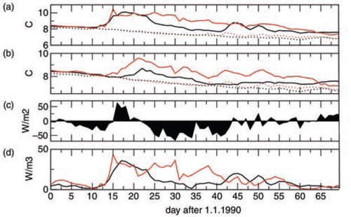
Accordingly, in the coupled model more heat remains in the ocean and is consequently transferred to depth which causes the stronger temperature increase at 72-m depth (Fig. 3b, red curve). Compared to this, the signal seen in the PC model is much weaker and delayed by a few days (Fig. 3b, black curve).

However, the heat exchange at the air–sea interface is more efficient than the vertical heat transfer within the water column, so one would expect the SST in the PCO model to be considerably lower than in the coupled model. In fact, the SST in the PCO model declines not before day 23 (Fig. 3a), that is, about 10 d after arrival of the T anomaly. The SST decrease in the ICO model is considerably slower because the water column remains more stratified compared with the PCO model (Fig. 3d, red curve), which keeps cooler water masses at depths. In contrast, the PCO model is already well mixed again (Fig. 3d, black curve). The fast declining SST then also reduces the heat loss at the air–sea interface (Fig. 3c) compared with the fully coupled model.

4.2. Basin wide anomaly

To obtain a more comprehensive analysis including all regional characteristics of the North Sea and Baltic Sea, we carried out experiments with applying a basin wide anomaly. In these experiments, the models were initialised with a temperature anomaly of +5 K in the upper 50 m and over the entire model domain. We here focus the question of how the added heat is dissipated between the ocean and atmosphere and if there is any long-term preservation of heat.

Figure 4a shows a time series of the volume integrated heat content. The anomaly is defined as the difference in heat content between the perturbed experiments and the unperturbed simulation. The North Sea loses the added heat rapidly in both model set-ups. Only a small amount of energy survives a complete seasonal cycle (~2.5%) at the end of the year. The slightly higher heat content anomaly in the ICO model in the first half of the year compared with the PCO model can be explained by the lower heat loss in the ICO model where the atmosphere warms likewise. In both models, 60–70% of the added heat is lost already during January and February. At this time, strong winds over the North Sea support a strong advective removal of the heat in the atmosphere (Kjellström et al., 2005). The damping feedback in the IC model is thus rather weak, and the difference between the two set-ups remains low and vanishes after 220 d (Fig. 4a).

Fig. 4 Heat content anomaly (difference of perturbation experiment minus unperturbed control run) calculated for the North Sea and Baltic Sea for: (a) the basinwide anomaly experiment and (b) the lateral boundary anomaly experiment. Red lines indicate interactive coupling. Black lines indicate passive coupling. Green lines in (a) indicate the difference between the red line and the black line.

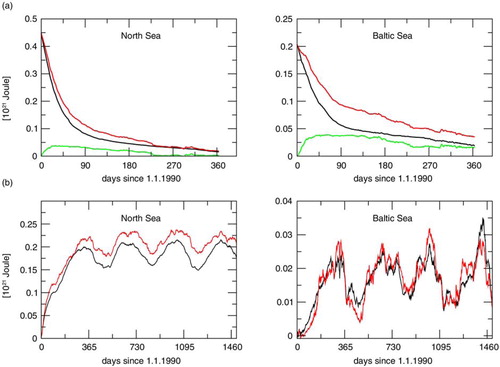
In the Baltic Sea, the ICO model shows a much smoother and less strong heat loss than the PCO model (Fig. 4a). Also, here the warming atmosphere damps the oceanic heat loss. However, in contrast to the North Sea, the Baltic Sea maintains a strong halocline during winter. Thus, more kinetic energy is necessary to mix the heated surface waters to layers below the halocline where they can be preserved for longer. In the ICO model, this process is much more efficient because the winds over the Baltic Sea are stronger than in the PC model. This is due to a positive feedback loop, that is, during winter the imposed SST anomaly and the successive warming of air destabilises the atmosphere, which results in stronger winds in the PC model compared with the ICO model. The result is an overall increase of wind stress, which operates only in the ICO model (Fig. 5a). The PCO model likewise exhibits a slight increase in wind stress. This is related to the changed surface circulation as the wind stress is calculated from the difference of 10 m wind velocity and velocity of the surface current. But this effect is by far lower than the dynamic effect of interactive coupling.

Fig. 5 (a) Difference in effective wind stress between the basinwide anomaly experiment and the unperturbed control run. Left: interactively coupled model. Right: passively coupled model. (b) Difference in effective wind stress between lateral boundary anomaly experiment and the unperturbed control integration. Top: Average over the last year of model integration (1994). Bottom: Average over June, July and August of the last year of model integration.

5.3. Lateral boundary anomaly

In this experiment, the lateral boundary temperatures were permanently increased by 5 K along the northern boundary as well as in western model boundary between England and France. The anomaly was applied from the water surface to the bottom. This set-up is similar to a warming Atlantic, which might occur in response to future climate warming.

Figure 4b shows the evolution of volume integrated heat contents for the respective model and basin. The North Sea adapts quite rapidly to the new boundary conditions. Already after 2 yr, no significant long-term heating trend is seen (Fig. 4b). This is in agreement with the vigorous cyclonic circulation in the North Sea (Winther and Johannessen, 2006). The difference between the two set-ups is most pronounced during winters (~20%) when the ocean to atmosphere heat transfer is highest. In the Baltic Sea, which is very remote from the perturbation source, the resulting heat anomaly is only about one-tenth compared to the anomaly in the North Sea (Fig. 4b). No significant difference is seen between the two model set-ups.

Figure 5b shows the impact of the added heat energy on the wind stress in the two set-ups. Also here, the wind stress increases substantially in the North Sea due to the destabilising effect on the atmosphere in the ICO model. Similarly, the effect is strongest in the vicinity of the inflow areas and weakens with increasing distance from the model boundaries. The effect is strongest during the cold season. However, the increased wind stresses over the North Sea are seen throughout the whole year (Fig. 5b, top) even during summer (Fig. 5b, bottom) when the North Sea takes up heat from the atmosphere (and cools it) imposing a stabilising influence on it. In fact, the oceanic heat uptake is lower in the perturbed simulation because SSTs are higher and the stabilising cooling influence of the North Sea is weaker. This effect is strongest in the deeper parts of the northern North Sea where a strong thermocline develops during the summer months. The presence of this thermocline operates like a thermostatic control of atmospheric winds in North Sea: During convective wind events, the mixed layer deepens and cooler subthermocline waters reach the surface. The resulting cooling of the sea surface then stabilises the atmosphere again. In the vicinity of the heat source, however, the surface cooling is much weaker and the stabilising effect lower.

The PCO model lacks the described interactive ocean–atmosphere feedbacks and its sensitivity to temperature perturbations is thus, much weaker (Fig. 5b).

5. Impact on mean climatologies

5.1. Winter

The perturbation experiments have shown that interactive coupling profoundly impacts on the air–sea heat exchange due to the interactive warming of the atmosphere influencing the heat exchange directly and due to associated changes in wind stress feeding back on the mixed layer thickness and thus on the vertical transfer of heat within the water column. The latter process is also important for the long-term heat uptake of the ocean and may thus become important in climate warming scenarios as it alters the distribution of heat between the ocean and the atmosphere.

We now investigate the importance of interactive coupling for the simulation of mean summer and winter temperatures. For this, we evaluate the two model set-ups with respect to the surface temperature climatology from the BSH observations.

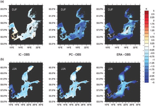
In a first step, we compare the simulated winter SST for the Baltic Sea and North Sea with observations. The PCO model is clearly too cold by 1.5–2 K in most areas of the Baltic Sea (Fig. 6) and by more than 3 K in the Skagerrak. In contrast to this, the coupled model is only slightly too cold with deviations below 0.5 K in most areas. Deviations only in the Skagerrak exceed 0.8 K.

Fig. 6 Comparison of simulated SST in the Baltic Sea with interactive coupling (left), passive coupling (middle) and the ERA40 SST (right) used as lower boundary condition for the atmosphere only simulation. Displayed is the difference to the observed climatology of the BSH (model minus observation).

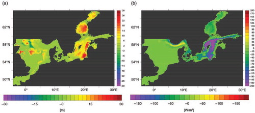
Responsible for the large bias of the PCO model is the quality of atmospheric forcing fields from the uncoupled atmosphere run (Fig. 2). Figure 6a (right) clearly indicates that the ERA40 SSTs that served as lower boundary condition for this run have a profound cold bias compared with the observations. The too cold SSTs have two effects: (1) they reduce the ocean to atmosphere heat fluxes thus making the atmosphere too cold and (2) in turn the associated stabilisation of the atmosphere weakens atmospheric winds. Hence, in the PCO run, the too cold atmosphere then enhances the ocean heat loss and the too weak winds create a too shallow mixed layer compared to the IC model (Fig. 7a). The latter is associated with weaker upward mixing of warmer deep waters which, in turn, amplifies the cold bias of the PC model. As a result, the potential energy anomaly, that is, the energy required to instantaneously homogenise the water column (Simpson and Bowers, 1981), is much higher in the PC model.

Fig. 7 Difference between the ICO minus PCO simulation in winter mixed layer thickness (a) and potential energy anomaly (b; Simpson and Bowers, 1981). Mixed layer thickness was calculated according to the 0.03 kg/m³ criterion (de Boyer Montegut et al., 2004).

In the North Sea, the ERA40 SST have lower biases than in the Baltic Sea (Fig. 8a, right) and so the PCO simulation performs much better with cold biases mostly below 1 K. However, the too cold Baltic Sea surface waters are advected into the northern North Sea along the outflow stream from the Baltic (Fig. 8a, middle). The ICO simulation performs overall well in the North Sea with deviations from the observed climatology below 0.75 K in most regions.

Fig. 8 Comparison of simulated SST in the North Sea with interactive coupling (left), passive coupling and the ERA40 SST used as lower boundary condition for the atmosphere only simulation. Displayed is the difference to the observed climatology of the BSH (model minus observation).

5.2. Summer

In summer, the two model set-ups perform equally well in both the North Sea and the Baltic Sea (Fig. 6b and 8b). This indicates that the interactive coupling is not so important as this is the case for the winter climatology.

Remarkably, the strong cold bias of the summer ERA40 SSTs in the Baltic Sea (Fig. 6b) has no substantial negative influence on the simulated SST in the PCO model as this is the case in winter. This is because during summer a pronounced thermal stratification develops and the oceanic capability to absorb heat from the atmosphere then strongly depends on the mixed layer thickness. On the one hand, the too cold atmosphere tends to cool the ocean in the PCO model as well. On the other hand, too weak wind stress inherited from the uncoupled atmosphere only run PCA (Fig. 2) reduce vertical mixing, which applies a positive effect on SSTs. In the PCO model, the two feedbacks largely counteract each other. In addition to that, the too low ERA40 SSTs reduce the cloud fraction over the sea. All this keeps the SST bias small. The largest differences occur near the eastern British coast and in the Kattegat where the SST is too cold by up to 3 K. But this is independent from the coupling technique indicating deficiencies in the ocean/atmosphere GCM.

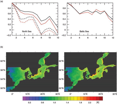
However, despite the good performance of the two model versions, we found substantial differences with regard to their internal dynamic behaviour. To illustrate this, we have carried out a lead correlation analysis between the 10 m wind velocity and SSTs for two stations in stratified region in the Baltic Sea and the North Sea (Fig. 9). In the Baltic Sea, the IC model shows a significant low-frequency oscillation between positive and negative correlation coefficients within the first 200 h (Fig. 9, red curve). Hence, stronger winds lower the surface water temperatures, which last for about 30 h mainly by increasing the mixed layer thickness. After that, the cold sea surface imposes a stabilising effect on the atmosphere which in turn weakens the winds again and lowers the mixed layer thickness. This leads then to increasing temperatures between days ~50 and ~150. This characteristic behaviour is not well captured in the PCO model. There is only a negative relationship between the winds and SSTs indicating primarily that stronger winds cool the SSTs (or lower winds enable warming) by advective heat removal, whereas the feedback by the changing mixed layer is less pronounced than in the ICO model. This is probably the case because of the too weak winds caused by the too low ER40 SST in the atmosphere only run.

Fig. 9 Wind lead correlation analysis for a station in the Baltic Sea (17.9°W; 19.9°N) and a station in the stratified northern North Sea (3.2°W; 58.5°N). The lead correlation has been carried out on 6-hourly 10 m wind and SST data during June and July 1990. Red line indicates the interactively coupled run IC. Black line indicates the passively coupled run PC.

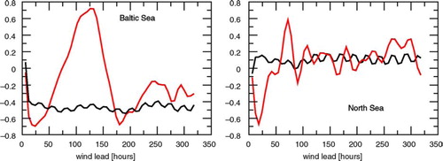
In the stratified North Sea, the coupled model ICO shows the same dynamical behaviour but the oscillation has a shorter period of only ~36 h than in the Baltic Sea, which has a period of ~150 h. The accelerated internal dynamics in the North Sea is in agreement with its lower stratification, which promotes a faster vertical energy exchange than in the stratified Baltic Sea.

6. Impact on thermal variability

6.1. Short-term interannual variability

Previous studies have shown that interactive coupling can considerably increase the variability of simulated SSTs, which can respond to changing air temperatures and thereby lowering air–sea heat fluxes (i.e. reduced thermal damping effect; Barsugli and Battisti, 1998; Bhatt et al., 1998; Saravanan, 1998; Fedorov et al., 2008). Moreover, it was found that the reduced air–sea heat fluxes can also result in a longer memory of the thermal conditions in the ocean. Bhatt et al. (1998) found a stronger (or longer) persistence of winter thermal anomalies in the North Atlantic when running the NCAR Community Climate Model in interactive mode. However, the strength of these effects is strongly tied to the wind conditions, that is, stronger winds tend to increase mixing in the ocean, which can result in higher air–sea heat exchange again (Sura and Newman, 2008) that negatively affects the ocean memory.

In the following, we analyse the potential memory effects for winter thermal conditions by correlating the monthly mean January heat content time series between 1990 and 2009 with the corresponding monthly mean times series for January, February, to December (Fig. 10a). In the well-mixed southern North Sea, the January thermal conditions influence the heat content notably only until June, whereas in the seasonally stratified northern North Sea, the influence lasts until October. Remarkably, in both models the correlation with October heat contents is higher than in September and August. This can be explained with the so-called re-emergence mechanism, which describes the phenomenon found in seasonally stratified regions that winter heat anomalies are sequestered beneath the shallow summer mixed layer and re-incorporated into the deepening fall mixed layer (Bhatt et al., 1998). During summer, the variability of the heat content is rather linked to the uptake from the atmosphere into the upper ocean layers, which is mainly independent from the preceding winter conditions. However, Fig. 10a indicates that the re-emergence mechanism is not amplified by the use of interactive coupling. Indeed, correlations are persistently higher in the passively coupled model and also the SST variability is not significantly higher in the IC model compared with the PC model (Fig. 10b). The only exceptions are the upwelling areas near the southern and southeastern Swedish coast. Hence, the effect of reduced thermal damping is not seen in these experiments. This can be explained by the dominance of higher wind velocities in the IC model compared to PC model, which increases vertical mixing, air–sea heat fluxes (Sura and Newman, 2008) and likewise the advective transport in the atmosphere.

Fig. 10 (a) Correlation between times series of monthly mean January heat contents with time series of monthly mean heat contents of other months. Red: interactively coupled model. Black: passively coupled mode. Dashed lines indicate the heat content of the well-mixed southern North Sea only (i.e. south of 54°N). (b) Standard deviation of daily mean SST time series (1990–1999). Note the seasonal cycle has been subtracted before analysis.

In the Baltic Sea, the memory for winter thermal conditions lasts until October in both models (Fig. 10a). The heat uptake during summer is weaker than in the North Sea and has no substantial influence on the variability of summer heat conditions as this is the case in the North Sea. A re-emergence mechanism is not seen probably because the Baltic has a strong halocline that prevents deeper layer to be incorporated into the mixed layer in winter as this is seen in the North Sea.

6.2. Long-term variations

An important question is: will the two model set-ups respond differently to a transient warming, as might be expected in the future? One might expect that semi-enclosed shallow shelf basins with restricted exchange with the open ocean will respond faster to climate warming, which makes them favourable for an early detection of climate change in a distinct region. Several studies have predicted an average SST increase for the North Sea between 1.5 and 2.0 for the downscaled SRES A1B Scenario (e.g. Adlandsvik, 2008; Holt et al., 2010; Gröger et al., 2013; Mathis and Pohlmann, 2014). However, all these studies have been carried out with either interactive or passive air–sea coupling leaving the question after sensitivity of projected warming to the coupling technique.

For the North Sea, a recent shift-like warming trend has been reported in literature especially after the 1980s (e.g. Harrison and Carson, 2007; Meyer et al., 2009; Emeis et al., 2014). Indeed, we see this warming trend also in our hindcasts (Fig. 11a). We do not aim to investigate the causes of the warming trend here. However, as the ocean model is driven by a fixed mean climatology at the open boundaries the only way to warm the North Sea is via the atmosphere (neglecting circulation-driven changes in heat transport). Hence, the warming trend is an ideal test case to study the effect of interactive coupling on the response to long-term atmospheric warming.

Fig. 11 (a) Annual mean SST averaged over the North Sea. Red line=interactive air–sea coupling (IC). Black line=passive air–sea coupling (PC). (b) Difference of annual mean SST between the PC minus the IC simulation. (c) Difference in volume integrated heat content between the PC minus the IC simulation.

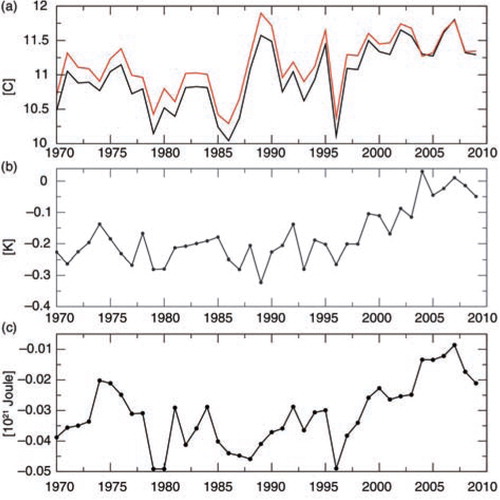
Figure 11b shows that the uncoupled model warms much faster than the coupled model, which reduces the cold bias of the uncoupled model compared to the coupled model at the end of the 20th century. To understand whether this different behaviour is only due to a different vertical redistribution of heat, we have calculated the 3-D heat content of the North Sea in the two set-ups (Fig. 11c). Indeed, it appears that during the last decade of the simulation the heat content evolves differently indicated by a faster increase seen in the uncoupled model. Hence, the uncoupled model responds faster/stronger to the warming atmosphere. The trends seen in Fig. 11 arise mainly from the summer and early autumn season (not shown), that is, when the North Sea experiences its strong thermal stratification. At this time, the water surface warming is highest. In the ICO simulation, the surface warming reduces the air-to-sea heat flux, so this ocean takes up less heat than in the PCO simulation. In both the ICO and PCO simulation, the sea surface warms and reduces the air-to-sea temperature difference (thereby reducing the air-to-sea heat flux), but only in the ICO model the atmosphere is cooled which additionally reduces the air-to-sea temperature difference and heat fluxes. Therefore, the ICO model takes up less heat than the PCO model (Fig. 11c).

This behaviour is similar to that deduced from the lateral boundary and basinwide perturbation experiments with the difference that additional heat is introduced via the atmosphere and not injected directly into the ocean's surface layer. The basinwide addition of heat was only instantaneous and the difference between ICO and PCO disappeared in this experiment already after 1 yr (Fig. 4a). By contrast, when adding heat persistently via the atmosphere and as done in the lateral boundary experiment, the coupling technique has a significant influence on the models response to heat perturbations. This will probably also alter the model results in case of long-term climate warming scenarios. However, to quantify this effect would require coupled and uncoupled scenarios.

7. Effects of interactive air–sea coupling on land atmospheric variables

We showed that interactive coupling profoundly influences the mean SSTs. And even if the simulated SSTs show similar results in the two set-ups, the coupled ocean–atmosphere dynamics can differ. We here briefly investigate whether interactive coupling can have long-distance effects over land. For this, we compared 30-yr (1970–1999) seasonal averages from both model set-ups.

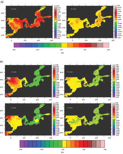
Figure 12a shows the difference of ICA minus PCA in simulated 2 m air temperature. The temperatures are generally warmer in the ICA model with the exception of the North Sea in winter. The differences are largest over the Baltic Sea where the too cold ERA40 SSTs translate into the atmosphere. We can further conclude that the biggest differences between the two model set-ups are more or less restricted to the actively coupled area, that is, the North Sea and Baltic Sea. Accordingly, statistically significant differences are only seen over the sea (Fig. 12a, right panels). Over land, the temperatures are mostly up to 0.2 K higher in the ICA model. Only around the Baltic Sea, the ICA model is warmer by up to 0.4 K.

Fig. 12 Difference between interactively coupled simulation and passively coupled simulation for winter (DJF) and summer (JJA): (a) 2 m air temperature and (b) precipitation. The right panel shows only differences that are significant at the 95% confidence level (tested with a two-sided t-test. The white line indicates the zero contour line).

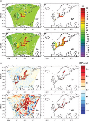
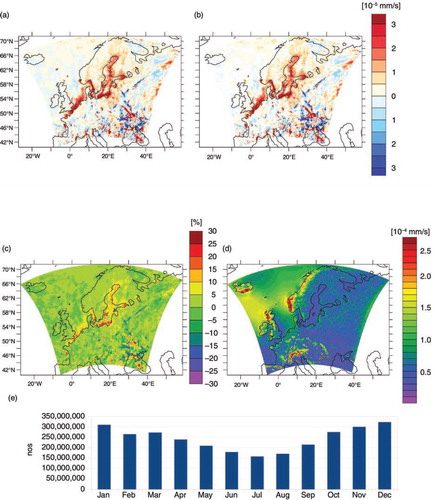
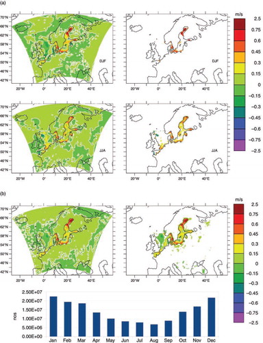
A similar result is seen in the simulated precipitation pattern (Fig. 12b). Over the Baltic Sea, the warmer air temperature in the ICA model enhances precipitation. During summer, increased evaporation over the Baltic strongly enhances precipitation also over the adjacent land areas especially in the eastern parts (Fig. 12b, lower panel left). But again, the changes are not statistically significant. To test the coupling effect on extrema, we compare only the highest 10% of precipitation sampled from outputs of every 15 min. The result is shown in Fig. 13. Most of the extreme values originate from the cold season (Fig. 13e). Also here, the largest difference occurs over the Baltic Sea. Although the differences are significant in a statistical sense (mainly owing to the high sampling size in the applied t-test, Fig. 13b), the overall magnitude of the differences is rather small. The highest differences occur over the Baltic Sea where the differences between the two set-ups can be up to 30% (Fig. 13c). In regions where extreme precipitation is highest, such as along the Norwegian coast, west Scotland and the Alps (Fig. 13d), the intermodel differences are surprisingly small.

Fig. 13 (a) Difference between interactively coupled simulation and passively coupled simulation for strong precipitation. Only precipitation above the 90% percentile was considered. (b) Difference above the 95% confidence level. (c) Relative differences expressed as percentage. (d) Absolute values of precipitation for the interactively coupled simulation and (e) distribution throughout the year of precipitation model outputs above the 90% percentile for the interactively coupled simulation.

The wind velocity 10 m above the surface also shows the strongest model differences over the Baltic Sea (Fig. 14a). This also relates to the too cold ERA40 boundary SSTs as noted already in Section 5 describing the effects on the mean ocean climatologies. Differences are especially pronounced over the Bothnian Bay in winter when lower sea ice concentrations in the ICA model promote a high heat loss of the ocean. Significant differences are seen also during summer when winds are rather weak and stable generating a low noise level in the significance test. As seen already in the 2 m temperature and precipitation, we find neither significant nor profound changes over land. This applies to both the seasonal mean averages and extreme values (Fig. 14b).

Fig. 14 (a) Difference between interactively coupled simulation and passively coupled simulation of 10 m wind velocity for winter (DJF) and summer (JJA). The white line indicates the zero contour line. (b) Same as (a) but considering only strong winds (above the 90% percentile). Also shown: distribution of strong winds throughout the year.

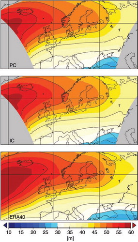
Another important climate sensitive pattern is the storminess over the North Atlantic and Europe, which is important in the ocean–atmosphere exchange of heat, water and momentum (e.g. Bengtsson et al., 2006). Earlier work has emphasised the sensitivity of storm track intensity to the sea surface temperatures in the North Atlantic and Europe (e.g. Woolings et al., 2010) as well as in the Pacific (O'Reilly and Czaja, 2014). Following earlier approaches of Sawyer (1970) and Blackmon (1976), we analyse the storm track intensity using 500 mb geopotential height field. Cyclones are the dominant source of variability in the frequency band of 2.5–6 d (Blackmon, 1976). Figure 15 shows the SD of the ICA and PCA modelled geopotential height in comparison to the ERA40 re-analysis data set which forced the simulations at the lateral boundaries. Storm track intensity over Europe is clearly underestimated by the RCA4 model. The weaker intensity is also independent of the used SST boundary condition, that is, also the higher winter SST over the Baltic Sea in the ICA simulation does not lead to a higher variability in the geopotential height field compared to the PCA simulation. Hence, in our experiments, the coupling technique has no profound influence on the storm track intensity. This is probably due to the relatively small area of interactive coupling (i.e. the North Sea and Baltic Sea) compared to the vast North Atlantic where storms arise from.

Fig. 15 Comparison of passively coupled (PC) modelled, interactively coupled (IC) modelled and ERA40 re-analysis geopotential height. Displayed is the standard deviation of analysed half-daily fields between 1990 and 1999.

8. Discussion and summary

Our experiments reveal that interactive coupling can significantly influence the simulated surface temperature in the North Sea and Baltic Sea. This includes also the dynamical behaviour of the processes that govern the distribution of heat between the atmosphere, the well-mixed upper ocean layer and the subpycnocline layers. We found interactive coupling most important during winter when strong winds force a tight coupling between the atmosphere and the deeper ocean layer. During summer, under strong thermal stratification interactive coupling is less important.

The PCO ocean simulation was too strongly tied to the prescribed atmospheric forcing from the PCA which itself was driven by a too cold ERA40 SST boundary condition. The too cold ERA40 SSTs translated into a too low T2m in the PCA experiments and further into too low SSTs in the PCO experiment. In addition to that, the low ERA40 surface temperature caused too weak winds in the PCA experiment, which in turn reduced the upward mixing of heat in the Baltic Sea thereby amplifying the PCO models cold bias. A comparison of ERA40 winds with the meteorological data set of the Swedish Meteorological and Hydrological Institute has shown that ERA40 winds are by up to 40% too low (Omstedt et al., 2005; Höglund et al., 2009).

In the ICO simulation, the involved processes, that is, mainly heat fluxes and atmospheric winds, were modelled more realistic, which resulted in our model also in a surface climatology much closer to observations than the PCO simulation. Of course, the better SST result of the ICO simulation cannot be related directly to the interactive coupling itself as the PCO model could be better tuned to compensate the too low T2m and the too weak winds. However, this would contemporaneously affect the models sensitivity, which would alter the models predictions in climate change scenarios.

Strictly speaking, our results explain only that the ICO simulation yields warmer winter surface temperatures compared to the PCO simulation and is much closer to the observational data set of the BSH.

The artificial perturbation experiments indicate that the distribution of heat between the atmosphere and the ocean is highly dependent on the coupling technique. In our experiments with positive temperature anomalies implemented in the ocean model, the feedback from the warming atmosphere reduced the sea to air heat fluxes thus more heat energy was transferred to deeper layers. As this feedback is not present in the PC model, an unrealistic high oceanic heat loss resulted in a substantial cooling of the sea surface.

Some of the mechanics of SST anomaly damping seen in the temperature perturbation experiments can be deduced already from the early work of conceptual models (e.g. Marotzke and Pierce, 1997; Nilsson, 2000) such as the distinction of different times scale in the context of SST anomaly damping. Figure 4a clearly shows that the two model set-ups exhibit an initial fast mode followed by a slowly mode of SST anomaly damping. In our more complex model (compared to the early conceptual models), the fast process is determined by the more advective time scale of the mixed layer response, whereas the slower mode relates to the more diffusive timescale of heat exchange between pycnocline wasters and subpycnocline waters. Although our experimental set-up differs profoundly from the early conceptual models from Marotzke and Pierce (1997) and Nilsson (2000), we clearly see the scale dependence of the SST anomaly damping. In the local anomaly experiment, both the ICO and PCO set-up show an almost complete vanishing of the SST anomaly after a bit more than 2 months compared to the unperturbed case (Fig. 3a) as in this case the atmospheric advection is efficient enough to transfer the heat far away. In the basinwide anomaly experiment, the atmospheric advection is no longer sufficient to remove the heat. This results in long-term preservation of heat in the ocean (Fig. 4a).

We have also found profound differences between the interactively and PCA runs, mainly caused by the different SST boundary condition and associated feedbacks. However, none of these changes significantly influence the atmospheric variables farther over land. On the one hand, this appears reasonable because of the different internal time scales of the ocean and the atmosphere. The ocean with its large heat capacity generates signals which are of low frequency and amplitude compared to the highly dynamic atmosphere over land, which is characterised by fast internal time scales due to low heat capacity of the land. Also, the fact that the ERA40 SST lacks the diurnal cycle (Fiorino, 2004) may damp the amplitude/frequency already over the ocean in the PCA run.

In contrast to our results, Van Pham et al. (2014) found large air temperature differences between the interactively coupled and the passively coupled version in the COSMO-CLM/NEMO ocean–atmosphere regional GCM over Europe. However, the authors reported the strongest changes far remote from the Baltic/North Sea region, that is, the interactively coupled area, whereas adjacent land areas appeared relatively unaffected by the coupling. This is contrary to our results, which indicate the influence of the coupling rather low and restricted close to the sea.

From our experiments, we can draw the conclusion that the added value of interactive air–sea coupling is twofold: (1) The problem of choosing an appropriate lower boundary condition is avoided and the SST, for example, the atmosphere PC run results from coherent physical processes and not from nudged re-analysis or highly interpolated observational data sets. Of course, the strong cold bias in the simulated winter SST using the PCO simulation can be reduced by employing a correction to the ERA40 SST. But the choice of any correction factor (which may be temporal and spatially highly variable) would introduce an additional source of uncertainty. Even worse, if one would try to tune model parameters, such as vertical mixing coefficients, etc., against a wrong boundary climatology.

The second benefit from interactive air–sea coupling is the elimination of the infinite energy source/sink term, which results from the lacking feedback of the prescribed boundary field during the simulation. In fact, this acts as an artificial restoring term for the dynamic model component, which cannot evolve as free as in the interactively coupled set-up. This restoring might be considered acceptable in re-analysis-driven simulations for the current climate as it prevents the model to drift too far from observed climatologies. For the downscaling of transient climate change simulations, however, this behaviour is inappropriate. In downscaling runs of GCM forced climate warming simulations, the ocean–atmosphere distribution of added heat would be determined too strongly by the driving GCM simulation. In this way, the interactively coupled model becomes more independent from the driving GCM simulation than the passively coupled. It is likely that this will reduce the spread of results in large downscaling ensembles, which make use of many different GCMs and scenarios. As a consequence, this can reduce uncertainties on the regional scale in future regional climate projections.

We here considered only the thermal aspect of interactive air–sea coupling. However, our result showed also quite large differences in the simulated precipitation over land between the IC and PC simulations (Fig. 12b). Although not reaching the level of statistical significance, in case of natural hazards, for example, river floods, where critical thresholds of accumulated water within a drainage basin play an essential role, small differences can also determine whether a flood occurs or not.

9. Acknowledgements

The research presented in this study is part of the Baltic Earth programme (Earth System Science for the Baltic Sea region, see www.baltex-research.eu/balticearth) and was funded by the Swedish Research Council for Environment, Agricultural Sciences and Spatial Planning (FORMAS) within the project – Impact of changing climate on circulation and biogeochemical cycles of the integrated North Sea and Baltic Sea system – (Grant no. 214-2010-1575) and from Stockholm University's Strategic Marine Environmental Research Funds Baltic Ecosystem Adaptive Management (BEAM). The simulations have been conducted on the Linux clusters Krypton and Triolith, both operated by the National Supercomputer Centre in Sweden (NSC). Resources on Triolith have been made available by the grants SNIC 2013/11-22 – Impact of changing climate on biogeochemical cycling in the North Sea and Baltic Sea region – and SNIC 2014/8-36 – Impact of changing climate on biogeochemical cycling in the North Sea and Baltic Sea region – part 2- provided by the Swedish National Infrastructure for Computing (SNIC).

References

- Adlandsvik B . Marine downscaling of a future climate scenario for the North Sea. Tellus. 2008; 60: 451–458.
- Barsugli J. J. , Battisti D. S . The basic effects of atmosphere–ocean thermal coupling on midlatitude variability. J. Atmos. Sci. 1998; 55: 477–493.
- Bengtsson L. , Hodges K. I. , Roeckner E . Storm tracks and climate change. J. Clim. 2006; 19: 3518–3543.
- Bhatt U. S. , Alexander M.-A. , Battisti D. S. , Houghton D. D. , Keller L. M . Atmosphere–ocean interaction in the North Atlantic: near-surface climate variability. J. Clim. 1998; 11(7): 1615–1632.
- Blackmon M. L . A climatological spectral study of the 500 mb geopotential height of the northern hemisphere. J. Atmos. Sci. 1976; 33: 1607–1623.
- Brown J. , Fedorov A. V. , Guilyardi E . How well do coupled models replicate the energetics of ENSO?. Clim. Dynam. 2011; 36: 2147–2158. DOI: 10.1007/s00382-010-0926-8.
- Christensen J. H. , Hewitson B. , Busuioc A. , Chen A. , Gao X. , co-authors . Solomon S. , Qin D. , Manning M. , Chen Z. , Marquis M. , co-editors . Regional climate projections. Climate Change 2007: The Physical Science Basis. Contribution of Working Group I to the Fourth Assessment Report of the Intergovernmental Panel on Climate Change. 2007; Cambridge: Cambridge University Press. 847–940.
- de Boyer Montegut C. , Madec G. , Fischer A. S. , Lazar A. , Daniele Iudicone D . Mixed layer depth over the global ocean: an examination of profile data and a profile-based climatology. J. Geohys. Res. 2004; 109: 1–20. DOI: 10.1029/2004JC002378.
- Dieterich C. , Schimanke S. , Wang S. , Väli G. , Liu Y. , co-authors . Evaluation of the SMHI coupled atmosphere-ice-ocean model RCA4_NEMO. SMHI-Report, RO 47. 2013. ISSN 0283-1112. Online at: http://www.smhi.se/polopoly_fs/1.28917!/RO_47.pdf .
- Donnelly C. , Andersson J. C. M. , Arheimer B . Using flow signatures and catchment similarities to evaluate the E-HYPE multi-basin model across Europe. J. Hydrol. Sci. 2015. DOI: 10.1080/02626667.2015.1027710.
- Donnelly C. , Arheimer B. , Capell R. , Dahne J. , Strmqvist J . Regional overview of nutrient load in Europe – challenges when using a large-scale model approach, E-HYPE. Understanding fresh-water quality problems in a changing world. Proceedings of IAHS-IAPSO-IASPEI Assembly. 2013; Sweden, IAHS Publ: Gothenburg. 361, 2013, pp. 49–58.
- Döscher R. , Meier H. E. M . Simulated sea surface temperature and heat fluxes in different climates of the Baltic Sea. AMBIO. 2004; 33(4): 242–248.
- Döscher R. , Willen U. , Jones C. , Rutgersson A. , Meier H , co-authors . The development of the regional coupled ocean–atmosphere model RCAO. Boreal. Environ. Res. 2002; 7(3): 183–192.
- Egbert G. D. , Erofeeva S. Y . Efficient inverse modeling of barotropic ocean tides. J. Atmos. Ocean. Technol. 2002; 19(2): 183–204.
- Egbert G. D. , Erofeeva S. Y. , Ray R. D . Assimilation of altimetry data for nonlinear shallow-water tides: quarter-diurnal tides of the Northwest European Shelf. Cont. Shelf Res. 2010; 30(6): 668–679.
- Emeis K.-C. , van Beusekoma J. , Calliesa U. , Ebinghausa R. , Kannenand A. , co-authors . The North Sea – a shelf sea in the Anthropocene. J. Mar. Syst. 2015; 141: 18–33. DOI: 10.1016/j.jmarsys.2014.03.012.
- Fedorov A. V , Goudie A. , Cuff D . Ocean–atmosphere coupling. Oxford Companion to Global Change. 2008; Oxford, Great Britain: Oxford University Press. 369–374.
- Feser F. , Rockel B. , von Storch H. , Winterfeldt J. , Zahn R . Regional climate models add value to global model data: a review and selected examples. Bull. Am. Meteorol. Soc. 2011; 92(9): 1181–1192. DOI: 10.1175/2011BAMS3061.1.
- Fiorino M . A multi-decadal daily sea surface temperature and sea ice concentration data set for the ECMWF ERA-40 reanalysis. ERA-40 Project Report Series No. 12. 2004; Reading, UK: European Centre for Medium-Range Weather Forecasts. 16 pp.
- Gröger M. , Maier-Reimer E. , Mikolajewicz U. , Moll A. , Sein D . NW European shelf under climate warming: implications for open ocean – shelf exchange, primary production, and carbon absorption. Biogeosciences. 2013; 10: 3767–3792. DOI: 10.5194/bg-10-3767-2013.
- Gustafsson N. , Nyberg L. , Omstedt A . Coupling of a high-resolution atmospheric model and an ocean model for the Baltic Sea. Mon. Weather Rev. 1998; 126(11): 2822–2846.
- Hagedorn R. , Lehmann A. , Jacob D . A coupled high resolution atmosphere–ocean model for the BALTEX region. Meteorol. Z. 2000; 9(1): 7–20.
- Harrison D. E. , Carson M . Is the world ocean warming? Upper-ocean temperature trends: 1950–2000. J. Phys. Oceanogr. 2007; 37: 174–187. DOI: 10.1175/JPO3005.1.
- Hasselmann K . Stochastic climate models Part I. Theory. Tellus. 1976; 28(6): 473–485.
- Höglund A. , Meier H. M. , Broman B. , Kriezi E . Validation and correction of regionalised ERA-40 wind fields over the Baltic Sea using the Rossby Centre Atmosphere model RCA3.0. Report Oceanografi 97. 2009; Norrköping, Sweden: SMHI.
- Holt J. , Wakelin S. , Lowe J. , Tinker J . The potential impacts of climate change on the hydrography of the northwest European continental shelf. Prog. Oceanogr. 2010; 86: 361–379.
- Hordoir R. , An B. W. , Haapala J. , Dieterich C. , Schimanke S. , co-authors . BaltiX: a 3D ocean modelling configuration for Baltic & North Sea exchange analysis. Report Oceanography 48. 2013; Norrköping, Sweden: SMHI.
- Jacob D. , Andrae U. , Elgered G. , Fortelius C. , Graham L. P. , co-authors . A comprehensive model intercomparison study investigating the water budget during the BALTEX-PIDCAP period. Meteorol. Atmos. Phys. 2001; 77(1–4): 19–43.
- Janssen F. , Schrum C. , Backhaus J. O . A climatological data set of temperature and salinity for the North Sea and the Baltic Sea. Dtsch. Hyrdrogr. Z. 1999; 51(Suppl. 9): 5–245.
- Janssen F. , Schrum C. , Hübner U. , Backhaus J . Uncertainty analysis of a decadal simulation with a regional ocean model for the North Sea and Baltic Sea. Clim. Res. 2001; 18(1/2): 55–62.
- Kerr R. A . Forecasting regional climate change flunks its first test. Science. 2013; 339: 638. DOI: 10.1126/science.339.6120.638.
- Kjellström E. , Bärring L. , Gollvik S. , Hansson U. , Jones C. , co-authors . A 140-year simulation of European climate with the new version of the Rossby Centre regional atmospheric climate model (RCA3). Reports Meteorology and Climatology 108. 2005; Norrkping, Sweden: SMHI. 54 pp.
- Kupiainen M. , Jansson C. , Samuelsson P. , Jones C. , Willn U. , co-authors . Rossby Centre regional atmospheric model, RCA4, Rossby Center News Letter. 2014. Online at: http://www.smhi.se/en/Research/Research-departments/climate-research-rossby-centre2-552/1.16562 .
- Kwon Y. O. , Deser C. , Cassou C . Coupled atmosphere mixed layer ocean response to ocean heat flux convergence along the Kuroshio Current Extension. Clim. Dynam. 2010; 36: 2295–2312. DOI: 10.1007/s00382-010-0764-8.
- Latif M. , Sperber K. , Arblaster J. , Braconnot P. , Chen D. , co-authors . The El Nio simulation intercomparison project. Clim. Dynam. 2001; 18(3–4): 255–276.
- Lehmann A. , Krauss W. , Hinrichesen H.-H . Effects of remote and local atmospheric forcing on circulation and upwelling in the Baltic Sea. Tellus A. 2002; 54: 299–316.
- Lehmann A. , Lorenz P. , Jacob D . Modelling the exceptional Baltic Sea inflow events in 2002–2003. Geophys. Res. Lett. 2004; 31(21): L21308.
- Liu Y. , Meier H. E. M. , Axell L . Reanalyzing temperature and salinity on decadal time scales using the Ensemble Optimal Interpolation data assimilation method and a 3D ocean circulation model of the Baltic Sea. J. Geophys. Res. 2013; 118(2013): 5536–5554. DOI: 10.1002/jgrc.20384.
- Löptien U. , Meier H. E. M . The influence of increasing water turbidity on the sea surface temperature in the Baltic Sea: a model sensitivity study. J. Mar. Syst. 2011; 88: 323–331.
- Madec G . NEMO Ocean Engine, User Manual 3.3. 2011; Paris, France: IPSL.
- Manabe S. , Stouffer R. V . Low-frequency variability of surface air temperature in a 1000-year integration of a coupled atmosphere–ocean–land surface model. J. Clim. 1996; 9: 376–393.
- Matei D. , Pohlmann H. , Jungclaus J. , Müller W. , Haak H. , co-authors . Two tales of initializing decadal climate prediction experiments with the ECHAM5/MPI-OM Model. J. Clim. 2012; 25: 8502–8523.
- Mathis M. , Mayer B. , Pohlmann T . An uncoupled dynamical downscaling for the North Sea: method and evaluation. Ocean Model. 2013; 72: 153–166.
- Mathis M. , Pohlmann T . Projections of physical conditions in the North Sea for the 21st century. Clim. Res. 2014; 61: 1–17. DOI: 10.3354/cr01232.
- Meier H. E. M. , Kauker F . Modeling decadal variability of the Baltic Sea: 2. Role of freshwater inflow and large-scale atmospheric circulation for salinity. J. Geophys. Res. 2003; 108(C11): 3368. DOI: 10.1029/2003JC001799.
- Meyer E. M. I. , Pohlmann T. , Weisse R . Hindcast simulation of the North Sea by HAMSOM for the period of 1948 till 2007 – temperature and heat content, GKSS reports 2009/3, ISSN 0344-9629, Helmoltzgemeinschaft, Geestacht. 2009. Online at: http://www.hzg.de/imperia/md/content/gkss/zentrale_einrichtungen/bibliothek/berichte/2009/gkss_2009_3.pdf .
- Marotzke J. , Pierce D. W . On spatial scales and lifetimes of SST anomalies beneath a diffusive atmosphere. J. Phys. Oceanogr. 1997; 27: 133–139. DOI: 10.1175/1520-0485(1997)027¡0133:OSSALO¿2.0.CO;2.
- Mikolajewicz U. , Maier-Reimer E . Mixed boundary conditions in ocean general circulation models and their influence on the stability of the model's conveyor belt. J. Geophys. Res. 1994; 99: 22633–22644. DOI: 10.1029/94JC01989.
- Nilsson J . Propagation, diffusion, and decay of SST anomalies beneath an advective atmosphere. J. Phys. Oceanogr. 2000; 30: 1505–1513. DOI: 10.1175/1520-0485(2000)030¡1505:PDADOS¿2.0.CO;.
- Omstedt A. , Chen Y. , Wesslander K . A comparison between the ERA40 and the SMHI gridded meteorological databases as applied to Baltic Sea modelling. Hydrol. Res. 2005; 36(4): 369–380.
- Omstedt A. , Elken J. , Lehmann A. , Lepparänta M. , Meier H. E. M. , co-authors . Progress in physical oceanography of the Baltic Sea during the 2003–2014 period. Prog. Oceanogr. 2014; 128: 139–171.
- O'Reilly C. , Czaja A . The response of the Pacific storm track and atmospheric circulation to Kuroshio Extension variability. Q. J. Roy. Meteorol. Soc. 2014; 141: 52–66. DOI: 10.1002/qj.2334.
- Samuelsson P. , Jones C. G. , Willén U. , Ullerstig A. , Gollvik S. , co-authors . The Rossby Centre Regional Climate model RCA3: model description and performance. Tellus A. 2011; 63: 423.
- Saravanan R . Atmospheric low-frequency variability and its relationship to midlatitude SST variability: studies using the NCAR climate system model. J. Clim. 1998; 11(6): 1386–1404.
- Sawyer J. S . Observational characteristics of atmospheric fluctuations with a time scale of a month. Q. J. Roy. Meteorol. Soc. 1970; 95: 610–625.
- Schrum C . Regionalization of climate change for the North Sea and Baltic Sea. Clim. Res. 2001; 18(1–2): 31–37.
- Schrum C. , Hübner U. , Jacob D. , Podzun R . A coupled atmosphere/ice/ocean model for the North Sea and the Baltic Sea. Clim. Dynam. 2003; 21(2): 131–151.
- Sein D. , Mikolajewicz U. , Gröger M. , Fast I. , Cabos W. , co-authors . Regionally coupled atmosphere – ocean – sea ice – marine biogeochemistry model ROM. Part I: Description and validation. J. Adv. Model. Earth Syst. 2015; 7: 268–304. DOI: 10.1002/2014MS000357.
- Seo H. , Miller A. J. , Roads J. O . The Scripps coupled ocean-atmosphere regional (SCOAR) model with applications in the Eastern Pacific sector. J. Clim. 2007; 20: 381–402.
- Simpson J. H. , Bowers D . Models of stratification and frontal movement in shelf seas. Deep-Sea Res. 1981; 28: 727–738.
- Su J. , Sein D. V. , Mathias M. , Mayer B. , O'Driscoll K. , co-authors . Assessment of a zoomed global model for the North Sea by comparison with a conventional nested regional model. Tellus A. 2014; 66: 23927. doi: http://dx.doi.org/10.3402/tellusa.v66.23927 .
- Sura P. , Newman M . The impact of rapid wind variability upon Air–sea thermal coupling. J. Clim. 2008; 21: 621–637. DOI: 10.1175/2007JCLI1708.1.
- Sun D.-Z. , Zhang T. , Covey C. , Klein S. A. , Collins W. D. , co-authors . Radiative and dynamical feedbacks over the equatorial cold tongue: results from nine atmospheric GCM. J. Clim. 2006; 19: 4059–4074.
- Tian T. , Boberg F. , Bssing Christensen O. , Hesselbjerg Christensen J. , She J. , co-authors . Resolved complex coastlines and land–sea contrasts in a high-resolution regional climate model: a comparative study using prescribed and modelled SSTs. Tellus A. 2013; 65: 19951. DOI: 10.3402/tellusa.v65i0.19951.
- Uppala S. M. , Kallberg P. W. , Simmons A. J. , Andrae U. , da Costa Bechtold V. , co-authors . The ERA-40 re-analysis. Q. J. Roy. Meteorol. Soc. 2005; 131: 2961–3012.
- Valcke S. , Caubel A. , Declat D. , Terray L . OASIS3 Ocean Atmosphere Sea Ice Soil Users Guide. 2003; CERFACS, Toulouse, France: Technical Report TR/CMGC/03-69.
- Vancoppenolle M. , Fichefet T. , Goosse H. , Bouillon S. , Madec G. , co-authors . Simulating the mass balance and salinity of arctic and antarctic sea ice. Ocean Model. 2009; 27: 33–53.
- Van Pham T. , Brauch J. , Dieterich C. , Frueh B. , Ahrens B . New coupled atmosphere–ocean–ice system COSMO-CLM/NEMO: assessing air temperature sensitivity over the North and Baltic Seas. Oceanologia. 2014; 56(2): 167–189. DOI: 10.5697/oc.56-2.167.
- Wang S. , Dieterich C. , Döscher R. , Höglund A. , Hordoir R. , co-authors . Development of a new regional coupled atmosphere–ocean model in the North Sea and Baltic Sea. Tellus A. 2015; 67: 24284. doi: http://dx.doi.org/10.3402/tellusa.v67.24284 .
- Watanabe M. , Kimoto M . Atmosphere–ocean thermal coupling in the North Atlantic: a positive feedback. Q. J. Roy. Meteorol. Soc. 2006; 126: 3343–3369. DOI: 10.1002/qj.49712657017.
- Weisse R. , von Storch H. , Callies U. , Chrastansky A. , Feser F. , co-authors . Regional meteorological–marine reanalyses and climate change projections: results for Northern Europe and potential for coastal and offshore applications. Bull. Am. Meteorol. Soc. 2009; 90(6): 849–860.
- Winther N. G. , Johannessen J. A . North Sea circulation: Atlantic inflow and its destination. J. Geophys. Res. 2006; 111: 12018. DOI: 10.1029/2005JC003310.
- Woolings T. , Hoskins B. , Blackburn M. , Hassel D. , Hodges K . Storm track sensitivity to sea surface temperature resolution in a regional atmosphere model. Clim. Dynam. 2010; 35: 341–353. DOI: 10.1007/s00382-009-0554-3.
- Zhang C . Madden-Julian oscillation. Rev. Geophys. 2005; 43: 1–36. DOI: 10.1029/2004RG000158.