The dynamic and thermodynamic structure of monsoon low-pressure systems during extreme rainfall events

Abstract

A cyclone-tracking algorithm is used to identify monsoon low-pressure systems (LPS) in the ERA-interim re-analysis (1979–2010). The LPS that are connected to observed extreme rainfall events are picked out and studied with a focus on their dynamic and thermodynamic structure. Cyclone composite clearly shows the general structure of the LPS, with a pronounced cold core at lower levels and warm core aloft. Evaporative cooling from the falling precipitation is proposed to generate the cold core. The temperature gradients across the cyclone centre are strongest in the early phase of the low. We suggest the baroclinic instability to be important in the development phase of the LPS, whereas the upward motion ahead of the low is maintained through latent heat release in the mature phase. This cooperation between the large-scale flow and the cumulus convection is known as the conditional instability of second kind (CISK). From the composites of the time steps where the extreme precipitation is occurring, a colocation of the strong updraft and vertical velocity is shown. Based on this, we suggest the extreme rainfall events to be a result of the LPS dynamics, which is dominated by the CISK mechanism at this stage of the low. Correlation and co-variability between the LPS precipitation and different meteorological parameters are performed, and we find the LPS precipitation to show a large sensitivity to variability in the vertical velocity and specific humidity at 750 hPa.

• monsoon low-pressure systems
• extreme precipitation
• cyclone tracking
• regression analysis

1. Introduction

The South Asian monsoon circulation, which is present over India normally from the beginning of June to the end of September, releases up to 70% of the total annual rainfall in India (Webster and Fasullo, 2003; Tyagi et al., 2012). Several synoptic scale systems are embedded in the large-scale monsoon circulation, and they are all a factor in the precipitation distribution over the Indian continent. One of the most important synoptic features is the monsoon low-pressure system (LPS). The LPSs develop over India and the adjoining ocean, propagate in a west–northwestward direction and release a large amount of precipitation over central India (Mooley, 1973; Goswami et al., 2003; Krishnamurthy and Shukla, 2007; Jadhav and Munot, 2009; Ajayamohan et al., 2010; Krishnamurthy and Ajayamohan, 2010). Monsoon LPS is a common name for these cyclonic storms, and the Indian Meteorological Department categorise them by the strength of the systems. The monsoon Low and monsoon depressions are the two most commons ones, where the monsoon Low is a less intense storm than the monsoon depression [see Sikka (2006) for a comprehensive description of the monsoon LPS].

The Indian monsoon region is characterised by strong vertical wind shear, which is a result of the large-scale monsoon circulation. The mean low-level flow is westerly and becomes easterly around 500 hPa (e.g. Shukla, 1978). The vertical extent of the monsoon LPS is up to 400 hPa, with a vorticity maximum around 800 hPa (Godbole, 1977). Thus, it could be expected that the LPS would be advected to the east by the low-level westerly winds, but the LPSs are rather propagating towards the west–northwest, against the mean flow. From a composite of five monsoon depressions, Godbole (1977) showed how the low-level convergence is mainly in the west–northwestward sector relative to the low-pressure centre and used this to explain the west–northwestward propagation of the systems. The reason for the low-level convergence and the corresponding strong updraft ahead of the low-pressure centre is still a highly relevant research topic, where several mechanisms have been proposed. Boundary layer friction, warm air advection, vorticity advection and cumulus processes are all triggering factors that can lead to the upward motion that is associated with a monsoon LPS (Sikka, 2006; Tyagi et al., 2012). Whereas friction has the largest effect in the upper part of the boundary layer, contribution of the other processes is a more complicated research question. The importance of the baroclinic process for the development of the depressions was emphasised by Saha and Chang (1983), where they described how the monsoon LPS has a well-defined area to the west of the cyclone centre, with warm-air advection from the north, and to the east of the cyclone centre there is cold-air advection from the south. By analysing the thermal budget of a monsoon depression, Saha and Saha (1988) suggested that even though the temperature advection is very small, it could be contributing to the initiation of vertical motion. Shukla (1978) highlighted the importance of the combination of the barotropic–baroclinic instability and the conditional instability of second kind (CISK; Charney and Eliassen, 1964) for the development of the depressions. They suggested that the primary driving mechanism for the growth of the monsoon depressions is the CISK theory, which is a cooperate feedback between the low-level convergence of the large-scale flow and the latent heat of condensation. Sanders (1984) diagnosed the quasi-geostrophic stream function and found vorticity advection and vortex stretching to account for the low-level divergence to the west of a depression centre. Chen et al. (2005) proposed a link between the diabatic heating and a divergent circulation in the east–west direction of the depressions, which is just another way of describing the CISK mechanism. They explain how the upward branch west of the depression centre is maintained through latent heat release, generating vortex stretching, allowing the depression to propagate westward. Even though not all the details about the low-level convergence and the strong upward branch west of the centre of the low are completely understood, it leaves no doubt that latent heat release is important for the intensification of the monsoon LPS (i.e. Saha and Saha, 1988; Shukla, 1978; Chen et al., 2005). The importance of latent heat is also strengthened through the colocation of the precipitation and the strong upward motions, reported by different studies (e.g. Godbole, 1977; Tyagi et al., 2012).

During the monsoon, there are on average 14 LPSs developing (Sikka, 2006). Goswami et al. (2003) and Krishnamurthy and Shukla (2007) revealed that there are more LPSs developing in the active period than the break period of the monsoon, where the active period is characterised by more precipitation over central India than during the break. Goswami et al. (2003) also found that the path of the LPS during the active period is clustered along the monsoon trough, and therefore the central Indian region receives more precipitation from these systems than compared to the rest of the continent. That the central Indian region gets much of its precipitation from the monsoon LPS was also noted by Krishnamurthy and Ajayamohan (2010). They performed a composite study of the rainfall associated with the LPS, and the analysis showed that during days when the LPSs are present (LPS days), central, southwest and northern part of India receive up to 10 mm more precipitation each day, than compared to the rest of the Indian subcontinent. Meanwhile, during days when there are no LPS present, southeast and northeast India receive approximately 10 mm more precipitation each day [see Fig. 3 in Krishnamurthy and Ajayamohan (2010)].

The monsoon LPSs are associated with large rainfall rates. Around the low-pressure centre, there is a cold anomaly at lower levels, and Shukla (1978) proposed the cold core to be the result of evaporative cooling from falling precipitation. The strong rainfall rates associated with the LPS can also turn into hazardous events; thus, the LPSs are often connected to extreme rainfall events in the central Indian region (i.e. Goswami et al., 2006; Sikka, 2006; Pattanaik and Rajeevan, 2010; Tyagi et al., 2012). The LPS can trigger intense rainfall events in the vicinity of the path of the low, or they may cover a large region and persist for a long time period, which results in the release of a large amount of precipitation over a greater area (Jadhav and Munot, 2009). Several studies suggest that there has been an increase in extreme rainfall events over India in recent decades (e.g. Sen Roy and Balling, 2004; Goswami et al., 2006; Rajeevan et al., 2008; Krishnamurthy et al., 2009). The increase in the extreme rainfall events in the central Indian region is connected to a change in the frequency distribution the monsoon LPS, noted by multiple studies (Jadhav and Munot, 2009; Ajayamohan et al., 2010). More extreme rainfall events can lead to an increase in flooding and landslides that will have a large impact on the millions of people living in this very dense populated country. Thus, to understand the development of the extreme rainfall events triggered by the monsoon LPS is essential for adaption and mitigation purposes, but also to complete the understanding of the meteorological conditions leading to these events.

In this article, we study the monsoon LPS over India and investigate the thermo-dynamical and dynamical structures of the systems, focusing on which meteorological parameters are important for the precipitation. We investigate the sensitivity of the parameters important for the precipitation associated with the monsoon LPS during an extreme rainfall event. We primarily use the re-analysis data set ERA-Interim (Dee et al., 2011); however, the satellite-based Tropical Rainfall Measuring Mission (TRMM; Huffman et al., 2007) is used for comparison, in addition to the gauge-based daily gridded rainfall data set from the Indian Meteorological Department (Rajeevan et al., 2006). The time period of the study is 1979–2010. Motivated by previous studies where tropical cyclones have been identified and studied (Bengtsson et al., 2007a), we investigate whether a similar method could be used to detect the monsoon LPS. The method is based on a cyclone-tracking algorithm (Hodges, 1994, 1995, 1999), and by performing sensitivity tests we discovered that it is not straightforward to develop an objective procedure to identify the systems. This is described in Section 2, together with the method of connecting the LPS to extreme rainfall events. By using the information on the time and position of the different LPS, composite and statistical analyses of the LPS are performed. These results give a statistical model with several predictors that together explain a large fraction of the variability in precipitation intensity associated with the monsoon LPS. All results are described in Section 3. We end with a summary and discussion of the main findings. An on-going work is to perform high-resolution climate sensitivity simulations of some of these LPS. This work will be presented in its own manuscript in the near future.

2. Data and methods

This study examines the precipitation associated with the monsoon LPS, with emphasis on the cases that give extreme precipitation. The data used are the ERA-Interim re-analysis (Dee et al., 2011) and the observation-based Indian Meteorological Department (IMD) precipitation (Rajeevan et al., 2006), with comparisons to the TRMM satellite precipitation (Huffman et al., 2007). The common time period for ERA-Interim and the IMD data sets is 1979–2010, and when we compare with TRMM we use the period 2000–2010. A brief summary of the data and methods will be given in the following subsections.

2.1. Identification of monsoon low-pressure systems

Monsoon LPSs are synoptic scale systems with a typical horizontal extent of 1000–2000 km, and a well-defined life cycle of 4–7 d. The thermal structure of the systems is cold cored at lower levels, becoming warm cored around 700–500 hPa (Sikka, 2006). The LPS develops in the Bay of Bengal, the Arabian Sea or over land and normally propagate in a northwestward direction (Saha et al., 1981; Yoon and Chen, 2005; Sikka, 2006; Krishnamurthy and Ajayamohan, 2010). The IMD categorise the LPS based on the wind strength, and the weaker lows are thought to cover a larger area and have a less intense precipitation rate than the deeper lows, which are known to release more precipitation over a smaller region (Ajayamohan et al., 2010). In this study, we will focus on all the storms that have the structure of a LPS. Hence, we use the common characteristics of the LPS to identify and find the path of the low. The procedure of detecting weather systems in data sets is a common technique to study the meteorological phenomena of interest (i.e. Yoon and Chen, 2005; Bengtsson et al., 2007a; Stowasser et al., 2009; Rudeva and Gulev, 2011; Pfahl and Wernli, 2012). Here, we use a Lagrangian-tracking algorithm that has been extensively used for detecting extratropical cyclones as well as tropical cyclones and mesoscale systems such as polar lows (Hodges, 1994, 1995, 1999; Bengtsson et al., 2007a; Kristiansen et al., 2011).

The algorithm is performed on the ERA-Interim data for the time period 1979–2010. The 850 hPa relative vorticity fields truncated to the spectral resolution of T42 for every sixth hour is used, and the feature points that exceed a vorticity threshold of 0.5×10⁻⁵ s⁻¹ are tracked and connected to a trajectory by minimising a cost function (Hodges, 1994, 1995, 1999). The trajectories, which travel a minimum distance of 5° and last for more than 48 h, are retained. Since relative vorticity is more pronounced in smaller scale features (Hoskins and Hodges, 2002), there are small vorticity maxima generated, which appear as tracking errors. It has been a common approach to remove these tracking errors by using a filtering method before applying the tracking algorithm (e.g. Anderson et al., 2003). However, we wish to detect all the features initially, and later filter out the falsely identified ones by introducing constraints comparable to the structure of the LPS systems.

After the features are identified in the relative vorticity field, we introduce two more criteria based on characteristics of the monsoon LPS: (1) a search for a true mean-sea-level pressure (MSLP) minimum in the vicinity of the track and (2) identification of the systems with a vertical thermal structure like monsoon LPS (i.e. cold core at lower levels and warm core aloft). For the MSLP minimum search, we use the full resolution ERA-Interim MSLP every 6 h, with a search radius around the trajectory for a surface pressure minimum of 5°. The MSLP minimum must be present for four consecutive time steps. To test the thermal structure, we adopt the procedure as in Bengtsson et al. (2007a), but instead of searching for tropical cyclones, which are warm cored systems throughout their whole vertical extents, the feature must have the thermal structure of a monsoon LPS, which are cold core at lower levels and warm cored aloft. The vorticity truncated to T63 at the pressure levels 850, 600, 500, 400, 300 and 250 hPa is used to test the thermal structure. The feature points from the trajectories that are identified in the T42 vorticity are used as a starting point, and first the T63 850 hPa relative vorticity maximum must exceed an intensity threshold of 1×10⁻⁵ s⁻¹. Next, a search of vorticity maximum at each level up to 250 hPa is performed, and only the tracks with a vorticity maximum within a 5° search radius at all the pressure levels is picked out. The vorticity maxima are then used to test the thermal structure of the systems along the trajectories. For a cold core (warm core) system, the vorticity increases (decreases) with height, and hence the vorticity difference between the lower and upper layer is larger (smaller) than zero. The cold core is tested between the pressure levels 850 and 500 hPa, and the warm core between 500 and 250 hPa. We used the least rigid choice of the vorticity difference threshold to ensure that the difference is positive (negative) for the cold (warm) core layer and does not exceed a prescribed threshold. The cold/warm core is required to be present for one time step during the LPS lifetime.

We limit our analysis to the monsoon, that is, from June to September. We also remove trajectories that develop above high orography, which may be a result of extrapolated values in the re-analysis. Since the LPS most commonly move in a northwestward direction, we pick out the ones that propagate in a northwestward direction. We also identify the trajectories that are inside the latitude/longitude covering 10–30°N and 65–100°E, which is the same region used in previous studies, the monsoon LPS (e.g. Sikka, 2006). Applying the algorithm on the whole time period and using all the criteria described above leave us with 133 systems during the 32 yr of study. A summary of the criteria is listed in Table 1. The track density, which shows the average number of trajectories in a 2.5°×2.5° grid box during the monsoon season, is shown in Fig. 1.

Fig. 1 The track density is showing the trajectories obtained from the algorithm, where the average number of trajectories during the monsoon season (LPS) is counted within a 2.5° square box. The time period used is 1979–2010.

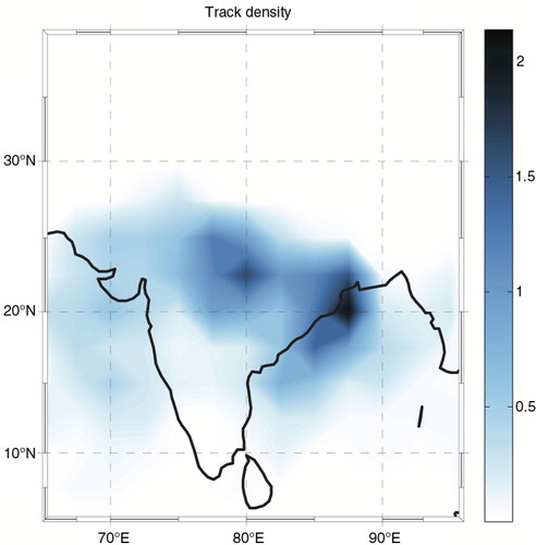
Table 1. All the different criteria used to detect the monsoon LPS in the ERA-interim re-analysis data set by using the automated tracking algorithm

Criteria
Vorticity intensity	The T42 relative vorticity at 850 hPa>0.5×10^−5 s^−1
Lifetime and displacement	Minimum 5° displacement during the lifetime. The minimum lifetime is 48 h (8 time steps)
A true MSLP minimum	A MSLP minimum (within a radius of 5° around the feature points) must exist for at least four consecutive time steps
Cold/warm core	The T63 850 hPa relative vorticity maximum needs to exceed a vorticity threshold of 1×10^−5 s^−1, and a vorticity maximum must exist at the levels 850, 600, 500, 400, 300 and 250 hPa within a 5° search radius. To test the thermal structure, the vorticity difference in the lower layer (850–500 hPa) is required to be positive, which indicate a cold core. The vorticity difference between the upper layers (500–250 hPa) must be negative, indicating a warm core. This must be true for one time step
Topography	All the trajectories that developed above 700 m are removed, which may be a result of extrapolated values in the re-analysis
Direction of movement	Northwestward direction
Season	The monsoon season (JJAS)
Area of study	Latitude 10–30°N and longitude 65–100°E

To evaluate the results from the automated tracking method and tune the different criteria, we compared our trajectories with trajectories in the Sikka data set (Sikka, 2006). The Sikka data set consists of statistics of the position and time duration of monsoon LPS that developed over India and the adjoining oceans from 1984 to 2003, and is constructed by analysing synoptic weather charts of the MSLP and the surface wind speed. Based on these two parameters, the monsoon LPS has been classified into a low, depression, deep depression, cyclonic storm or severe storm. There are several challenges with applying an automated tracking algorithm to detect the monsoon LPS in a re-analysis data set. Initially, we thought by introducing more and more constraints, we would remove the tracking errors and the small-scale disturbances, and eventually be left with the strongest systems, i.e. the depressions. The average number of trajectories detected in each season is 4.2, which is lower than the long-term average number of depressions of seven per season (Godbole, 1976; Sikka, 2006), but in the same order as found in Hurley and Boos (2014) (four depressions per season) and around two depressions more than found by Sikka (2006) for the time period 1984–2003. In the Sikka (2006) data set, there are in total 274 LPS (on average 13.7 LPS each season), where 45 are categorised as depressions or deep depressions (2.25 each season). The coincidence of the trajectories found by our method and with the observed trajectories found in Sikka (2006) is very good; however, we realised we were left with not only depressions but also weaker systems known as monsoon Lows. Hence, we cannot state that this method is capable of detecting the climatology of the depressions, but it leave us with a data set of monsoon LPS that have developed during similar meteorological conditions, since they have the same thermal structure. The difficulty of removing the tracking errors to reproduce the climatology is something that should be further tested. Hurley and Boos (2014) developed a climatology of monsoon LPS by using the same tracking algorithm as used here, but with different constraints. Even though their seasonal average numbers was not far from the seasonal average numbers of monsoon LPS found in Sikka (2006), they found very little correlation between the interannual variations in the two data sets. Thus, to compare a climatology constructed with different methods from two different data sets is perhaps not trivial. For instance, when we introduced the cold/warm core criteria, the number of trajectories detected became very sensitive to this criterion. The method used in Sikka (2006) to pick out the LPS is based on an inspection of a synoptic pressure chart, where they identify the lows in a MSLP chart. It is not necessarily the case that all the LPSs found by Sikka (2006) have the cold/warm core structure, and this may explain why we have a much lower number of monsoon LPS than found by Sikka (2006). In spite of this, we wanted to include the cold/warm core criteria, since it is successful at removing the tracking errors and leave us with a sample of LPS cases we can with similar thermal structure that makes a composite analysis more sound.

2.2. Extreme precipitation

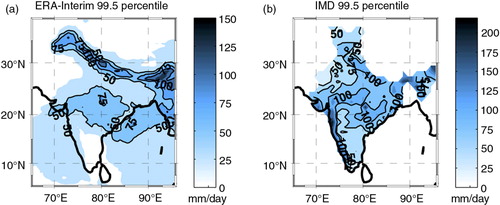
The next step is to investigate if there is extreme precipitation associated with the LPS. An extreme precipitation event is defined as an event that exceeds the 99.5th percentile, where the percentile is calculated at each grid point. Using precipitation from the re-analysis ensure that the trajectories and precipitation are physically consistent. The ERA-Interim precipitation is a prognostic variable, and it is therefore thought to have a poor skill, especially in the tropics where convective precipitation is dominated. However, a study by Lin et al. (2014) found that the ERA-Interim is the re-analysis data set that shows the highest skill in reproducing the climatology of the monsoon precipitation, and this increases our confidence in using the re-analysis precipitation. Despite this, there is still a large uncertainty in the precipitation, and we want to identify the precipitation events in the ERA-Interim that give us the most confidence. We, therefore, include another precipitation data sets, which is the observationally-based high-resolution daily gridded rainfall data from the IMD (Rajeevan et al., 2006). If we assume the IMD rainfall data to have the best performance when it comes to the precipitation over India, and use that data set as the ‘truth’, we can pick out the extreme rainfall events that are present in both ERA-Interim and the IMD rainfall data sets. By doing so, we are left with the events that we have most confidence in. The disadvantage of using IMD is that it only covers India; thus, we do not get any information about the skill of ERA-Interim over the ocean or the neighbouring countries of India, which also may be affected by these systems. Since IMD is thought to have the best skill when it comes to precipitation over India, and since we are mainly interested in how these extreme events may affect the people, the ocean is not the focus of this study. The procedure of finding the extreme events is as follows: First, we use the daily accumulated precipitation from IMD and ERA-Interim to find the common extreme rainfall (CER) events. The IMD (ERA-Interim) precipitation has a horizontal resolution of 1°×1° and is valid at 03 UTC (0.5°×0.5° and 12 UTC), respectively. The 99.5th percentile of the daily precipitation for the summer months (JJAS) for the time period 1979–2010 was calculated at each grid point for the two data sets and can be seen in Fig. 2. Note that the ERA-Interim underestimates the extreme values compared to the IMD. That ERA-Interim underestimates the extreme precipitation is also noted in previous studies (Pfahl and Wernli, 2012). For the 99.5th percentile, there are 20 events at each grid point during the 32 yr, and this makes on average 0.62 events each season. We first find the extreme events in the IMD precipitation. Then, the ERA-Interim 16 h before and 9 h after are compared. Because of the different horizontal resolution of the two data sets, the precipitation in the ±0.5 degree grid points in ERA-Interim is compared with the IMD rainfall. If one of the nine grid points exceeds the given percentile, the event is picked out. We call this a CER event. There are large spatial differences in how often there is agreement between the two data sets, where the coincidence is mainly around 15–20% (not shown). Thus, if the IMD data set represents the ‘truth’, ERA-Interim reproduces the timing and/or location of the extreme rainfall events poorly. One reason for this limited representation of the extremes in ERA-Interim may be due to the uncertainty regarding the convection parameterisations. However, there are also uncertainties in the representation of the extremes in observation-based gridded data, since extremes often are confined to be very local phenomena. Thus, the interpolation method, number of rain gauge data within the grid square and the horizontal resolution of the gridded data will all affect the quality of the precipitation data set. Therefore, it is likely that the intensity of extremes is not appropriately reproduced in the IMD data either.

Fig. 2 The 99.5 percentile of daily precipitation calculated for (a) ERA-Interim re-analysis and (b) IMD daily rainfall for the time period 1979–2010. The 50, 75 and 100 mm/d contours are shown in black. Note the different colour bars.

2.3. Connecting the common extreme rainfall events with a LPS

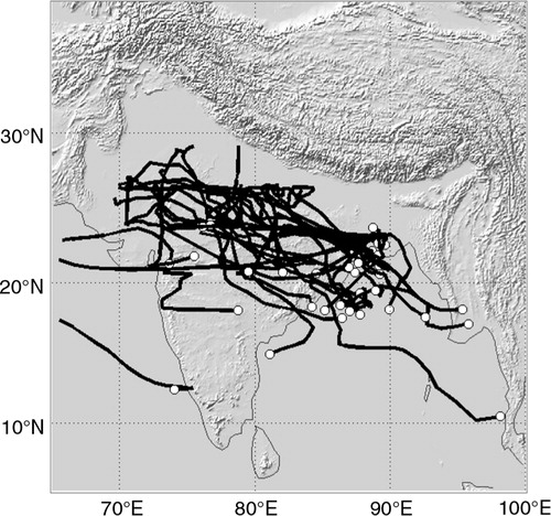
The next step is to find out if the CER is related to the passage of the LPS. The trajectories are interpolated to a 1 h time step, and an influence area of 5° around the centre of the low for each time step of the LPS is selected. Since the daily IMD rainfall is accumulated over the last 24 h, we only check if the CER lies within the influence area of the LPS during the last 24 h. If that is the case, we say that the extreme rainfall event is connected to the LPS. This results in 39 LPS trajectories, and the path of the trajectories can be seen in Fig. 3. We use as a criterion that there has to be an extreme rainfall event in the IMD data set and, therefore, the LPSs are confined to the Indian subcontinent.

Fig. 3 The LPS trajectories that are related to an extreme rainfall event for the time period 1979–2010, with regard to the different criteria. The white circles indicate the start position of the LPS. The grey shading indicates the topography. See text for a further explanation.

3. Results

Our data set consists of trajectories of 39 LPS that develop during 1979–2010 over the Bay of Bengal and the area nearby India, and are connected with an extreme rainfall event (defined by the 99.5th percentile) over the Indian subcontinent. To investigate the structure of these systems, a composite analysis is performed on different parameters that are of interest, with data from the ERA-Interim re-analysis data set for every 6 h. The composite methodology uses a radial coordinate system centred on the low-pressure centre (calculated from the vorticity maximum at 850 hPa), and rotated in the direction of propagation of the low-pressure system for each time step. The same method has been used in previous studies (i.e. Bengtsson et al., 2007b; Azad and Sorteberg, 2014). The composite is divided into two: when the LPSs are located over land and when the LPSs are located over ocean. This gives us the advantage of investigating different stages of development, where the ocean composite can be interpret as the formation stage, and the land composite is the mature/dissipation stage. In addition, for each LPS, the time step when the precipitation exceeds the 99.5th percentile is also picked out, and a composite of when there is extreme precipitation (P_max) is constructed (if there are more than one event for each LPS that exceeds the 99.5th percentile, the time step with the largest precipitation magnitude and that is closest to the cyclone centre is selected). With data every 6 h, there are 1019 samples when all the time steps from the 39 LPS are summarised, 793 samples when the LPS are located over land, 226 samples when the LPS are located over ocean and 39 samples for the extreme precipitation. The 1019 samples every 6 h gives an average lifetime of 6.5 d for each LPS.

In addition to the composite analysis, different statistical analyses are performed. Correlations are calculated by correlating the 6-hourly spatial averages within a radius of 5° around the low-pressure centre with the different parameters in ERA-Interim. Since we have selected the LPS that generate extreme rainfall events over land, the statistic is most representative for the LPS that results in high amounts of rainfall over land. The statistical significance of the correlation coefficients is computed by using a two-tailed t-test, and the level of significance is 99%.

3.1. Cyclone composite

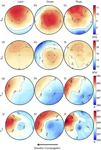
The cyclone composite shows the general features of the low-pressure systems and is, therefore, a good way to investigate different meteorological parameters. We choose the following meteorological parameters: MSLP, omega at 750 hPa (ω₇₅₀), 6-hourly accumulated precipitation, temperature at 750 hPa (T₇₅₀) and 950 hPa (T₉₅₀), and the specific humidity at 750 hPa (q₇₅₀) and 950 hPa (q₉₅₀). The composite with a 10° radius around the low-pressure centre is shown in Figs. 4 and 5, and we show the composite for the land, ocean and P_max composite. The deep surface low pressure is clearly seen in the centre of the MSLP composite, with no large differences between when the system is over land (Fig. 4a) and when the system is over ocean (Fig. 4b). The magnitude of the surface low is 3–4 hPa lower for the time step when the maximum precipitation occurs (Fig. 4c) than for the composite over land and ocean. The vertical velocity, ω₇₅₀ (ω is negative for upward motions), is mainly upward over the whole domain, with very strong upward motion ahead of the surface low. This area of strong upward motion is larger over ocean (Fig. 4e) than over land (Fig. 4d). For the time step with maximum precipitation, there is very strong upward motion slightly to the north, northwest and northeast of the low-pressure centre, but the total area of upward motion is decreased (Fig. 4f).

Fig. 4 Composite results of LPS-related MSLP (upper row; a–c), ω ₇₅₀ (middle row; d–f) and 6 h accumulated precipitation (bottom row; g–i) for the period 1979–2010. The column to the left shows the composite over land, the middle column shows the composite over ocean and the right column shows the composite for the time of maximum precipitation. The direction of movement is from east to west. Note that negative (positive) ω is upward (downward) motions.

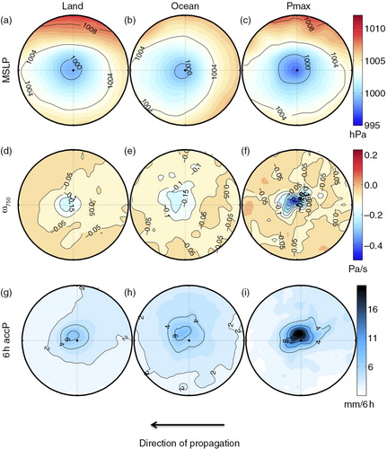
Fig. 5 Same as Fig. 4, but for the parameters q ₇₅₀ (a–c), q ₉₅₀ (d–f), T ₇₅₀ (g–i) and T ₉₅₀ (j–l).

The 6 h accumulation of precipitation shows a clear maximum ahead and to the northwest of the centre of the low, and the precipitation maximum is located close to the location of the maximum vertical velocity, corresponding to previous results (e.g. Godbole, 1977; Tyagi et al., 2012). The area where there is precipitation is also larger when the LPSs are over ocean (Fig. 4h) than over land (Fig. 4g), as is also seen for ω₇₅₀. These findings coincide well with the results of Romatschke and Houze (2011). They did a study with the TRMM Precipitation Radar (PR), where they divide the total precipitation into precipitation system size and find that the larger convective systems release more precipitation over the Bay of Bengal and Arabian Sea, while the smaller and medium-sized systems release more precipitation over land. For the time steps when the maximum precipitation occurs, there is a great increase in the amount of the 6-hourly precipitation compared to the other time steps (Fig. 4i).

The composites of the specific humidity at 750 and 950 hPa clearly show a decrease in the humidity with increasing altitude. Even though an accumulation of humidity at 750 hPa around the low-pressure centre is evident, composites over land (Fig. 5a), over ocean (Fig. 5b) or for the composites of the maximum precipitation (Fig. 5c) have different structures. Over land (Fig. 5a) and for P_max (which is predominantly over land, Fig. 5c), there is a maximum in the specific humidity mainly to the north of the low-pressure centre, while over ocean the maximum humidity is more symmetric around the centre of the low (Fig. 5b). The same features can be seen for the specific humidity at 950 hPa (Fig. 5d–e), but then the gradient in the humidity across the low-pressure centre is weaker, with the exception of the composite over ocean, where there is a strong decrease in the humidity to the northeast of the centre of the low.

From the temperature composites (Fig. 5g–l), we can see that there is a zone with warm air ahead of the low, and a colder region behind the low centre, and this structure is seen from lower levels up to 750 hPa. The temperature gradient across the cyclone centre is larger at 950 hPa than at 750 hPa, where at lower levels the difference between the warm zone and the cold zone is up to 5–6 K, while only 3–4 K aloft. The temperature at 750 hPa for the different composites looks very similar, except for the temperature at the time step for maximum precipitation. The temperature ahead of the cyclone centre for this composite is 1–2 K larger than for the other composites. Since there is much precipitation at this time, the higher temperature can be explained by the release of latent heat due to condensation.

The cold core at lower levels and warm core aloft is also clearly seen. The cold core over ocean is more defined than over land, where both the cold and warm air section covers a larger area. This gives a stronger temperature gradient across the cyclone centre in the composite over ocean than in the land composite. The cold core associated with the monsoon LPS is well documented in previous studies (e.g. Godbole, 1977; Sikka, 2006). In the P_max composites of the temperature in 950 hPa, the cold core is more pronounced than for the other composites. To see if the cold core can be a result of evaporative cooling of the precipitation, a simple estimate is calculated. The evaporative cooling is given as in the following:$C_p{\rho }_{a}H\frac{dT}{dt}=\epsilon PL,$

where c _p is the specific heat at constant pressure (c _p =1004 Jkg⁻¹ K⁻¹), ρ _a is the density of air (ρ _a =1.25 kg m⁻³), H is the thickness of the layer where the cooling is occurring, L is the latent heat of vaporisation (assumed as a constant L=2.4×10⁶ Jkg⁻¹), P is the precipitation rate, ɛ is the fraction of the precipitation that evaporates and dT/dt is the change in temperature with time. We use the average values of the temperature at 950 and 750 hPa (as is seen in Fig. 5) to obtain the thickness of the layer (calculated from the hypsometric equation by using the virtual temperature). In addition, the precipitation rate is the average 6-hourly precipitation seen in Fig. 4. If 10% of the falling precipitation is evaporating (ɛ=0.1), we calculate a cooling of 0.6 K/6 h. From Fig. 5, we see that there is a temperature difference between the cold core and the warmer air surrounding it in the range of 0.5–2 K each 6 h. Hence, if there is 10–30% evaporation of falling rain, a large fraction of the cold core at the lower level can be explained by evaporative cooling.

The strong temperature gradients at lower levels are distinct in the different composite results; hence, it seems likely that the warm air advection is playing an important role for the cyclone development. Saha and Chang (1983) investigated two monsoon depressions and showed that to the west of the depression there is strong upward motion and warm air advection, while to the east of the depression there is downward motion and cold air advection. This baroclinic advection induces a secondary circulation, with convergence (divergence) at lower levels and divergence (convergence) aloft to the west (east) of the low. From the composites, we see that there is a warm zone ahead of the low-pressure and a cold air zone behind the low-pressure centre, which correspond to the baroclinic advection described in Saha and Chang (1983). The strong upward motion is also seen in the composites from the ERA-Interim re-analysis data. However, we do not see the corresponding downward motion to the east of the low-pressure centre. Thus, these results suggest that it is not the baroclinic advection that is the main reason for the upward motion. Since the precipitation maximum and the strong vertical upward motions are collocated, the latent heat release due to condensation is most likely intensifying the strong upward motion, following the CISK mechanism. Shukla (1978) suggested this cooperation of the low-level synoptic convergence with cumulus convection to be the main driving mechanism for the growth of a monsoon depression. The east–west circulation across the low-pressure centre shown by Saha and Chang (1983) was further investigated by Chen et al. (2005), where they proposed the latent heat release to maintain the upward branch of the circulation. Since the temperature gradients are stronger in the ocean composite than in the land composite, this can be interpreted as stronger temperature advection in the early phase of the low, than in the later phase of the lows lifetime. Based on this, we suggest the barotropic–baroclinic instability to be important in the early phase, where temperature advection may play a role in initiating the upward velocity ahead of the low-pressure centre. The CISK mechanism becomes more important in the later phase of the low, where the release of the latent heat becomes important to maintain the upward motion, shown by the colocation of the maximum precipitation and strong upward velocity. However, we want to emphasise that this should be studied in more detail by analysing the physical processes that develop and drive the LPS.

3.2. Comparing ERA-Interim precipitation with TRMM precipitation

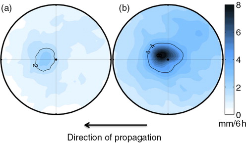
According to the literature, the precipitation from the monsoon low-pressure systems is located to the west–southwest of the surface low (Saha and Saha, 1988; Sikka, 2006). The precipitation from ERA-Interim is placed more to the west–northwest of the surface low. To see if this structure in precipitation is seen in different data sets, we calculate a composite of the precipitation from TRMM for the low-pressure systems that developed from 2000 to 2010 (14 cases and 307 sample time steps in total), and the composite is not divided into land/ocean composites, but all the time steps are considered. The comparison between the composite of TRMM and ERA-Interim is seen in Fig. 6. The magnitude of the precipitation is lower for TRMM than ERA-Interim, but it is clear that the precipitation from the satellite-based estimates is placed more to the west–southwest of the low-pressure centre, which coincides better with what is seen in previous studies. Moreover, both precipitation data sets have a precipitation tail that expands to the northeast of the cyclone centre. The spatial correlation of the mean precipitation in a 5° radius around the low-pressure centre between TRMM and ERA-Interim is 0.61. From Fig. 2, we see that ERA-Interim underestimates the extreme values compared to observations, yet ERA-Interim produces too much precipitation compared to TRMM, which suggests that ERA-Interim is overestimating the total amount of precipitation within the LPS. However, the low precipitation rate in TRMM compared to ERA-Interim could also be a result of the fact that the path of the low coincides better with the precipitation from ERA-Interim than the TRMM precipitation.

Fig. 6 Comparison of the 6 h accumulated precipitation from TRMM (a) and ERA-Interim (b) for the composite from all time steps.

3.3. A physically motivated statistical model linking LPS precipitation to other meteorological parameters

We want to identify different meteorological parameters we can use to explain the precipitation variability associated with the LPS. The choice of parameters is based on a simple description of precipitation intensity neglecting microphysical delay (i.e. condensate falls out immediately). The evaporation of the falling rain depends on the change in the condensate with time and the vertical extent of the atmosphere where the condensation occurs. This may be approximated to be the thickness of the clouds that produce the condensate. A simple estimate for the bottom of the cloud is taken as being at the lifting condensation level. Hence, the precipitation can be approximated as$P\approx \{-\underset{P_{LCL}}{\overset{P_{top}}{\int }}\frac{d{q}_s}{dt}dp=\underset{P_{LCL}}{\overset{P_{top}}{\int }}\left(\frac{d{q}_s}{dT}\frac{dT}{dp}\frac{dp}{dt}\right)dp,\hspace{1em}\hspace{1em}\frac{d{q}_s}{dt}<0\hspace{1em}\hspace{1em}\hspace{1em}\hspace{1em}\hspace{1em}\hspace{1em}\hspace{1em}\hspace{1em}\hspace{1em}\hspace{1em}\hspace{1em}\hspace{1em}\hspace{1em}\hspace{1em}\hspace{1em}\hspace{1em}\hspace{1em}\hspace{1em}\frac{d{q}_s}{dt}\ge 0$

where q _s is the specific humidity at saturation, T is the temperature and p is the pressure. We see that the precipitation will depend on temperature (through Clausius–Clapeyron equation; dq _s/dT), the stability (dT/dp), the vertical velocity in pressure coordinate (dp/dt) and the relative humidity (RH) (through the level of the LCL).

The above simple reasoning suggests that to find statistical connections between precipitation and other meteorological parameters, we should start with investigating relations to temperature, stability, vertical velocity and RH. RH is given as the ratio between the specific humidity (q) and the saturated specific humidity (q _s), where q _s is directly related with the temperature. A better choice may be to use specific humidity (q) instead of RH, to avoid the meteorological parameters used in the statistical analysis being too interconnected. Thus, our starting point is that precipitation variability is linked to variability in vertical velocity, temperature, specific humidity and static stability:$P=P\left(\omega ,T,q,\frac{dT}{dP}\right)$

We select parameters in the lower and middle atmosphere as a proxy for the whole lower tropospheric column. Our initial estimate of the parameters is, therefore, the vertical velocity in pressure coordinates (omega) at 750 hPa, temperature and specific humidity at 950 and 750 hPa, and a simplified estimate of the stability by taking the temperature difference between 750 and 950 hPa (dT/dp). Hence, the statistical analysis is performed between the 6-hourly accumulated precipitations and the parameters ω ₇₅₀, T ₇₅₀, T ₉₅₀, q ₇₅₀, q ₉₅₀ and dT/dp. We focus on the composites land, ocean and P_max.

3.3.1. Correlation between different parameters.

We start by investigating the correlation between the different meteorological parameters identified above, as the correlations between the different parameters will be important for our interpretation of the statistical results. Table 2 lists the correlations between the parameters ω ₇₅₀, T ₇₅₀, T ₉₅₀, q ₇₅₀, q ₉₅₀ and dT/dp, for the three different composites. The strongest correlation is between the specific humidity at 750 and 950 hPa, where the correlation ranges from 0.77 (land) to 0.90 (ocean). Hence, to have more humidity aloft, it is necessary to have a large amount of humidity at lower levels. The vertical velocity at 750 hPa (ω ₇₅₀) is statistically significantly related to specific humidity (both in 750 and 950 hPa). Thus, strong upward motion leads to more humidity at both 950 hPa and 750 hPa. Since the upward vertical velocity is associated with low-level convergence, we see that to achieve high values of specific humidity at lower levels and aloft, low-level convergence is necessary. There is also a strong negative correlation between the temperature at 950 hPa and the lower troposphere static stability (dT/dp), ranging from −0.68 (land) to −0.84 (P_max), but the correlation between temperature in 750 hPa and the lower troposphere static stability is weak. This indicates that it is the temperature at lower levels rather that the temperature aloft controls the temperature difference parameter. The temperature at 750 hPa is, as expected, not only most correlated with T ₉₅₀, but also has a weak correlation with the specific humidity at 950 and 750 hPa, except for the time step when the maximum precipitation is occurring. Then, the correlation is not significant. From Table 2, we see that there is a good consistency between the different parameters from the ERA-Interim re-analysis data set, and that the correlations between the parameters correspond well to the expected physical behaviour of the different parameters.

Table 2. Correlations between the different ERA-Interim parameters (ω ₇₅₀, T ₇₅₀, T ₉₅₀, q ₇₅₀, q ₉₅₀, dT/dP) for the different composites: over land, over ocean and P_max.

		ω 750	T 750	T 950	q 750	q 950	dT/dp
ω 750	Land Ocean Pmax	1
T 750	Land Ocean Pmax	−0.09 0.12 0.07	1
T 950	Land Ocean Pmax	0.00 0.13 0.13	0.62 0.44 0.75	1
q 750	Land Ocean Pmax	−0.35 −0.55 −0.58	0.13 0.22 0.21	−0.07 0.04 0.02	1
q 950	Land Ocean Pmax	−0.30 −0.53 −0.59	0.14 0.35 0.32	−0.04 0.07 0.09	0.77 0.77 0.90 0.81	1
dT/dp	Land Ocean Pmax	−0.09 −0.04 −0.14	0.05 0.35 −0.27	−0.75 −0.68 −0.84	0.20 0.14 0.14	0.17 0.21 0.12	1

The composites are defined in Section 3. The values in bold are correlated at the 99% confidence level.

Table 3 lists all the correlations for the different composites with the ERA-Interim precipitation. They are all statistically significant at a 99% significance level, except for the correlation between precipitation and temperature at 750 hPa for all three composites (land, ocean and P_max) and for the correlation between precipitation and lower troposphere static stability (dT/dp) over ocean. The precipitation has the strongest correlation with omega in 750 hPa, ranging from −0.75 over the ocean to −0.60 over land; hence, when there is more precipitation, there are also strong uprising motions. The specific humidity is also important for the precipitation, and the moisture at 750 hPa has a higher correlation than the moisture at lower levels, where the correlation spans from 0.65 (0.57) for the extreme cases to 0.44 (0.38) for the composites over land for q ₇₅₀ (q ₉₅₀). The temperature difference has no significant correlation with the precipitation over ocean but is more important for the precipitation over land. There is no correlation between the temperature at 750 hPa and the precipitation close to the cyclone centre. During precipitation events, substantial amount of latent heat is released in the middle of the atmosphere, where the amount of the condensed water (and latent heat release) is proportional to the amount of precipitation (e.g. O'Gorman and Schneider, 2009). The latent heat release would lead to an increase in the temperature in the layer where there is condensation, and we would expect to see a correlation between the precipitation and the temperature in the middle of the atmospheric. However, cooling due to adiabatic ascent is also occurring, and through analysing of the thermal budget of a monsoon depression Saha and Saha (1988) showed that the adiabatic cooling offsets the latent heat release. This balance can explain the lack of correlation between the LPS precipitation and the temperature in 750 hPa. The temperature at lower levels is more important and has a weak negative correlation with the precipitation, spanning from −0.27 for the extreme cases (P_max) to −0.17 over land. Colder temperature at lower levels is related to more precipitation. This is tangibly a result of evaporative cooling of the air from the precipitation at lower levels that leads to cooling of the surface, as shown in Section 3.1.

Table 3. Correlations between the ERA-Interim precipitation for the different composites (land, ocean and P_max) with the different meteorological parameters (ω ₇₅₀, T ₇₅₀, T ₉₅₀, q ₇₅₀, q ₉₅₀, dT/dP), as well as the predicted precipitation from the multivariable linear regression model.

ERA-Interim precipitation	Over land	Over ocean	Pmax
ω 750	−0.60	−0.78	−0.75
T 750	0.03	−0.08	−0.05
T 950	−0.17	−0.20	−0.27
q 750	0.44	0.59	0.64
q 950	0.38	0.55	0.57
dT/dp	0.24	0.15	0.36
Predicted P	0.66	0.80	0.83

The composites are defined in Section 3. The values in bold are correlated at the 99% confidence level.

3.3.2. Multiple linear regression.

We have seen that the precipitation associated with the monsoon LPS is correlated with the parameters chosen based on a simple approximation of the precipitation. As seen in Table 3, the strength of the correlation varies, and the parameters ω ₇₅₀ and q ₇₅₀ are more strongly correlated with the precipitation than T ₉₅₀ and dT/dP, for instance, while there is no correlation between the temperature at 750 hPa and precipitation. Based on the correlations between the different parameters, we suggest the precipitation associated with the LPS to be a function of 750 hPa vertical velocity, 750 hPa specific humidity and the atmospheric stability (dT/dp), i.e. P=P (ω _750, q ₇₅₀, and dT/dp). If we approximate the function as the Taylor series, and remove all the non-linear terms, we are left with a first-order expansion of the Taylor series. This is the same as a multivariable linear model where the dependent variable is the precipitation and the predictors are ω ₇₅₀, q ₇₅₀, and dT/dp, given as the following:$P=\frac{\partial P}{\partial {\omega }_{750}}\mid {\omega }_{750}+\frac{\partial P}{\partial q_{750}}\mid q_{750}+\frac{\partial P}{\partial \frac{dT}{dP}}\mid \frac{dT}{dP}+b.$

The precipitation is the 6-hourly accumulated mean ERA-Interim precipitation within a 5° radius around the LPS at each time step. The predictors (ω ₇₅₀, q ₇₅₀, and dT/dp) are also taken as the mean within a 5° radius of the LPS, b is the intercept, and the local derivatives are the slopes of each predictor. There is one caveat by performing this statistical analysis; the predictors are not independent, as seen in Table 2. The correlation is strongest between the vertical velocity and the specific humidity at 750 hPa. The atmospheric stability shows no relation to the two other predictors.

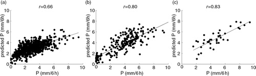
We perform the multivariable linear regression where we divide the parameters into the composites land, ocean and P_max. Scatterplots of the linear precipitation estimated and the re-analysis 6-hourly precipitation for the three composites are shown in Fig. 7. The correlation between the re-analysis precipitation and the predicted precipitation is 0.66 for over land, 0.80 for over ocean and 0.83 for the time step with maximum precipitation, and they are all statistically significant at a 99% confidence level (Table 3). The linear model reproduces 43–69% of the precipitation variability with only three variables from two different atmospheric levels. Thus, to get a good estimate of the LPS precipitation, variables from only a few levels in the atmosphere is required.

Fig. 7 Scatterplots with the best-fit regression line (solid line) between the ERA-Interim precipitation (x-axis) and predicted precipitation calculated with the multivariable linear regression model (y-axis). The composite (a) over land, (b) over ocean and (c) the P_max. The correlations are given in each sub-figure.

3.3.3. Importance of the different predictors in the statistical model.

With the statistical model, we can investigate the importance of the different predictors, and see how much the precipitation is altered if one of the predictors is changed. This must be done with caution, as we have already noted that the predictors are not independent. Table 4 summarises the sensitivities of precipitation to the different predictors from the linear regression model. For ω ₇₅₀ and q ₇₅₀, the precipitation sensitivities are given in%/10% (% change in precipitation per 10% change in ω ₇₅₀ or q ₇₅₀), while for the atmospheric stability the precipitation sensitivities are given in%/K (% change in precipitation per 1 K). The results from the sensitivities are only slightly different whether it is for the composite over land, over ocean or the time step with the maximum precipitation. A 10% change in ω ₇₅₀ gives a 4.3–5.0% change in the precipitation, while a 10% increase (decrease) in q ₇₅₀ gives an 8.3–10.8% increase (decrease) in the precipitation. Moreover, a 1 K change in dT/dp leads to 5.9–14.1% change in the precipitation. For comparison, a one standard deviation (σ) change in ω ₇₅₀ gives a change in the precipitation in the range of 27–54%, while one σ change in q ₇₅₀ gives a 13–19% change in the precipitation, where the ocean composite has the largest standard deviation for both ω ₇₅₀ and q ₇₅₀. One standard deviation of dT/dp is approximately equal to 1 K; thus, a precipitation change with one σ increase/decrease is approximately equal to a 1 K change. From the above, we see that it is the variability in vertical velocity that is influencing the precipitation the most.

Table 4. Sensitivity tests of the statistical model.

Sensitivity	Over land	Over ocean	Pmax
dP/dω 750 (%/10%)	4.3	4.5	5.0
dP/dq 750 (%/10%)	9.3	10.8	8.3
dP/(dT/dp) (%/K)	9.4	5.9	14.1

The change in precipitation (dP) if one of the predictors is changed [dω ₇₅₀ , dq ₇₅₀ , d(dT/dP)], for the different composites (land, ocean and P_max). The composites are defined in Section 3. See Section 3.3.3 for details.

3.4. The fit of the statistical model with TRMM precipitation

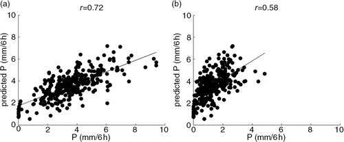
The statistical model presented can reproduce the ERA-Interim precipitation with a strong correlation. However, to see how the linear model fits with the TRMM precipitation, we compare the precipitation variability from the multivariable linear regression model with the TRMM precipitation by using the same time period and same LPS cases as described in Section 3.2 are used. Figure 8 shows the regression of the predicted precipitation by using the linear model, on the ERA-Interim (Fig. 8a) and TRMM (Fig. 8b) 6-hourly precipitation. The correlation between ERA-Interim (TRMM) and the predicted precipitation for this time period is 0.72 (0.58), and they are both statistically significant at a 99% significance level. Thus, the statistical model is capable of describing 34% of the precipitation variability in another precipitation data set with three parameters from only two levels in the atmosphere.

Fig. 8 The predicted precipitation calculated with the predictors from the regression model (y-axis), correlated with ERA-interim precipitation (a) and TRMM precipitation (b) (x-axis). The time period used is 2000–2010.

4. Summary and discussions

This study investigates the dynamical and thermodynamical structure of monsoon LPS that developed during the time period 1979–2010. By using a tracking algorithm (Hodges, 1994, 1995, 1999), the LPS are identified and tracked in the ERA-Interim re-analysis data set. The LPS that have an extreme rainfall event within an influence radius of 5° of the centre of the low are selected and analysed. An event is defined as extreme when the precipitation exceeds the 99.5th percentile in both the ERA-Interim re-analysis data set and the IMD daily rainfall. In total, 39 LPS cases fulfilled all the criteria. The main findings of the analysis of the LPS cases are discussed in the following.

Cyclone composites give a good visual picture of the structure of a low-pressure system. Godbole (1977) constructed composites of five different monsoon depressions of different meteorological parameters, and our results concur with his findings, where the general characteristics of the monsoon LPS is clearly seen in the composites. The deep surface low is distinct (Fig. 4a–c), and the thermal structure with a cold core at lower levels and warm core aloft is evident (Fig. 5g–l). The composites show a well-defined warm air sector ahead of the low, and a cold air region behind the low-pressure centre, and the temperature gradients across the lows are stronger in the early phase of the low than compared to the later phase. Strong upward velocity ahead of the surface low is seen in the composite, which is collocated with the maximum precipitation. The maximum precipitation and strongest updraft is covering a larger region over ocean than over land, and that precipitation systems have a larger horizontal extent over ocean than over land is confirmed by Romatschke and Houze (2011).

The structure and mechanism for the development and intensification of monsoon LPS have been studied in detail in previous studies (e.g. Shukla, 1978; Saha and Saha 1979; Saha and Chang 1983; Chen et al., 2005). The discussion leaves no doubt that the LPS are dependent on both baroclinic processes and the CISK mechanism; however, it is not clear which mechanism is the dominant one. Monsoon LPS are synoptic-scale systems, with organised deep convection around the centre of the low, which are characterised by mesoscale features. During the various stages of the low, different processes can be dominating for the LPS dynamics. In this study, we have not addressed the contribution from different processes; however, through visual inspections of the composites we propose the baroclinic instability to be important to initiate the upward velocity in the early phase of the low, and the CISK mechanism to be more dominant in in the later phase of the low, where the release of latent heat is maintaining the upward velocity. This argument is built on the findings of the stronger baroclinic zone seen in the low-level temperature composite in the early phase of the low (ocean composite), than compared to the later phase (land composite). Thus, we cannot see the secondary circulation induced by a baroclinic zone strengthens our suggestions. We only see the upward motion west of the low, but not the corresponding downward motion to the east. A pre-excising low-level convergence ahead of the low will be intensified through latent heat release due to condensation, which will support the stronger vertical velocities that again will lead to more condensation. This feedback loop will continue until there is a cut-off in the moisture supply or the upward motion is being suppressed. When the LPS makes landfall, the moisture source is tangibly going to be the limiting factor; therefore, the LPS will dissipate as it progress inland. This CISK mechanism seems to play an important role in intensification of the low, where the maximum precipitation and the strong upward vertical motion is co-located, particularly visible in the P_max composite (Fig. 4). A lower surface pressure is seen at the centre of the low for the P_max composite compared to the land and ocean composite. This is accompanied by a stronger pressure gradient and low-level convergence. Based on these arguments, the extreme rainfall events seem to be triggered by the synoptic LPS dynamics, which is primarily driven by the CISK mechanism at this stage.

We have investigated the relationships between the precipitation associated with the LPS and different meteorological parameters, and the correlations found correspond well to the expected physical behaviour. It is necessary to have low-level convergence that generates the upward motion so the air parcel rises adiabatically, the temperature cools and the parcel reaches saturation. In addition, there has to be significant amounts of moisture present. The LPS precipitation has the strongest correlation with the vertical velocity at 750 hPa, ranging from −0.6 (for the composite over land) to −0.78 (over ocean). However, the humidity at 750 hPa is also important, where the correlation ranges from 0.44 (over land) to 0.64 (P_max). The temperature at 750 hPa is not significantly correlated with the precipitation. The correlation between the precipitation and the simultaneous temperature should not necessarily be strong, since before the precipitation is initiated, the air parcel has to be lifted, experiencing adiabatic cooling before the condensation can occur, which would again lead to a warming of the layer. These two processes are shown to balance each other (e.g. Saha and Saha, 1988). The temperature at 950 hPa is significantly negatively correlated with the LPS precipitation, and this is explained by that the lower levels are cooled by the evaporation of the precipitation. We made a rough estimate of the evaporative cooling and found a cooling in the lower tropospheric column to be in the range of 0.5–2 K/6 h, corresponding to the cold core seen in the different composites. Thus, our results are in line with Shukla (1978) that suggested the cold core to be a result of evaporative cooling.

It has been shown that the precipitation in the west–southwest sector of monsoon depressions is maintained by convergence of moisture flux, i.e. $P~-\nabla ∆Q$ (Chen et al., 2005; Yoon and Chen, 2005). The divergence of moisture flux can be approximated as $\nabla ∆Q\approx \overrightarrow{\mathbf{V}}∆\nabla q+q\nabla ∆\overrightarrow{\mathbf{V}}$, and by assuming the horizontal gradient of the specific humidity (∇q) to be small compared to the wind divergence ($\nabla ∆\overrightarrow{\mathbf{V}}$), the moisture flux can be approximated as $\nabla ∆Q\approx \overrightarrow{\mathbf{V}}∆\nabla q+q\nabla ∆\overrightarrow{\mathbf{V}}$, where the continuity equation is integrated from the surface to some reference height Δz Based on this simple reasoning of the divergence of moisture flux, a relationship between the precipitation and the moisture flux convergence (given by the thickness of a layer, the vertical velocity and the specific humidity) is expected. Figure 4 shows a colocation of the strongest upward vertical velocity and the maximum precipitation, and in Fig. 5 it is shown that the specific humidity distribution is more uniform over a larger area, especially at lower levels. The moisture transport divergence should be calculated at all pressure levels to obtain an accurate estimate; however, from the visual inspection of Figs. 4 and 5, and from the correlations between the precipitation, vertical velocity and specific humidity, it is plausible to assume that the LPS precipitation is supported by the convergence of the moisture flux, as shown by Chen et al. (2005).

We found the atmospheric stability (taken as the temperature difference between 750 and 950 hPa; dT/dP), vertical velocity and specific humidity at 750 hPa to be the parameters that are most important for the precipitation variability. A multiple linear regression is, therefore, performed where the 6-hourly accumulated mean ERA-Interim precipitation is the dependent variable, and the predictors are the mean ω ₇₅₀, q ₇₅₀, and dT/dp. We developed a statistical model that diagnoses the precipitation associated with a LPS with fairly strong correlations ranging from 0.66 (precipitation over land) to 0.83 (P_max; Fig. 7 and Table 3). Since the statistical model assumes the predictors are independent, the results should be interpreted with care (Table 2 summarises how the different variables are correlated with each other). The statistical model shows that by choosing a small set of meteorological variables, we achieve a fairly good description of the precipitation associated with the LPS. Furthermore, with the statistical model we can make crude calculations of how sensitive the precipitation is to changes in the predictors. The model shows that if we increase the upward (downward) vertical velocity by 10%, 4.3–5% more (less) precipitation is produced. A 10% change in the specific humidity will lead to an almost equal percentage change in the precipitation. If we increase the temperature difference with 1 K (i.e. increasing the stability), the precipitation will increase in the range of 5.9% (ocean composite) to 14.1% (P_max composite). The sensitivity of the temperature stability is somehow misleading, since initially we would expect a reduction in the precipitation with an increase in the atmospheric stability. However, the temperature difference is mainly controlled by the lower atmospheric temperature, which is influenced by the evaporative cooling from the precipitation. This is evident from the sensitivities of the different predictors, where the P_max composite shows the largest increase in the precipitation with a change in the atmospheric stability. Thus, the large amount of the precipitation is the reason for the increase in the atmospheric stability due to the cooling at lower levels. This just emphasises that the interpretation of statistical models should be done with care, since the causation is not given by the correlations.

O'Gorman and Schneider (2009) derived a physical interpreted method to scale the precipitation extremes in idealised climate simulations. If the moisture is conserved, vertical moisture advection $\left(\omega ,·\frac{\partial \mathrm{qs}}{\partial p}\right)$ is balanced by the precipitation. From this scaling, we see that a change in the vertical velocity will change the amount of condensed water, and therefore the precipitation. The saturated specific humidity is only dependent on the atmospheric temperature; thus, this scaling will break down for analyses of case studies as we have performed here. The cold temperature anomaly generated by the precipitation will influence the scaling; thus, the results from the scaling will be opposite to what is the reality on the timescales of our analysis. The scaling derived by O'Gorman and Schneider (2009) is only meant for long-term climate studies where the temperature is representative of the climate and not influenced by temperature anomalies produced by single weather events.

In this study, we use data from the ERA-Interim re-analysis, and the results show that there is a good physical consistency between the different parameters. Even though it is shown by Lin et al. (2014) that the ERA-Interim precipitation has the highest skill in reproducing the monsoon climatology, we find that there is some shortage in the ERA-Interim performance when it comes to the rainfall associated with the monsoon LPS. When comparing the ERA-Interim precipitation with the TRMM precipitation (Fig. 6), we find that ERA-Interim produces too much precipitation during each time step and also the precipitation associated with the LPS is placed differently compared to the TRMM precipitation. Moreover, when comparing the extreme rainfall events with the extreme rainfall events in the observationally-based IMD data set, we see that ERA-Interim underestimates the extremes (Fig. 2), and often the extremes either develop in the wrong place or/and at the wrong time. Analysis of extreme weather events is best performed by using station data and not gridded data, since the number of stations in the grid box and the interpolation method will affect the extreme values. Thus, one should be cautious in interpreting the IMD gridded data as reality. However, in this study we use the data available to perform analyses in which we have the most confidence.

Acknowledgements

The authors are grateful to the National Climate Centre in Pune for sharing the IMD daily gridded rainfall data set; to Dr. Kevin Hodges, who provided and helped with the tracking algorithm; to Dr. Roohollah Azad and Dr. Ellen Viste for sharing programming codes and for informative discussions. The work was partly funded by Centre for Climate Dynamics at the Bjerknes Centre for Climate Research, University of Bergen and the Norwegian Research Council projects NorIndia and SnowHim.

References

- Anderson D. , Hodges K. I. , Hoskins B. J . Sensitivity of feature-based analysis methods of storm tracks to the form of background field removal. Mon. Weather Rev. 2003; 131: 565–573.
- Ajayamohan R. S. , Merryfield W. J. , Kharin V. V . Increasing trend of synoptic activity and its relationship with extreme rain events over central India. J. Clim. 2010; 23: 1004–1013.
- Azad R. , Sorteberg A . The vorticity budgets of North Atlantic winter extratropical cyclone life cycles in MERRA reanalysis. Part I: development phase. J. Atmos. Sci. 2014; 71: 3109–3128.
- Bengtsson L. , Hodges K. I. , Esch M . Tropical cyclones in a T159 resolution global climate model: comparison with observations and re-analyses. Tellus A. 2007a; 59: 396–416.
- Bengtsson L. , Hodges K. I. , Esch M. , Keenlyside N. , Kornblueh L. , co-authors . How may tropical cyclones change in a warmer climate?. Tellus A. 2007b; 59: 539–561.
- Charney J. G. , Eliassen A . On the growth of the hurricane depression. J. Atmos. Sci. 1964; 21: 68–75.
- Chen T. C. , Yoon J. H. , Wang S. Y . Westward propagation of the Indian monsoon depression. Tellus A. 2005; 57: 758–769.
- Dee D. P. , Uppala S. M. , Simmons A. J. , Berrisford P. , Poli P. , co-authors . The ERA-Interim reanalysis: configuration and performance of the data assimilation system. Q. J. Roy. Meteorol. Soc. 2011; 137: 553–597.
- Godbole R. V . The composite structure of the monsoon depression. Tellus A. 1977; 29: 25–40.
- Goswami B. N. , Ajayamohan R. S. , Xavier P. K. , Sengupta D . Clustering of synoptic activity by Indian summer monsoon intraseasonal oscillations. Geophys. Res. Lett. 2003; 30(8): 1431.
- Goswami B. N. , Venugopal V. , Sengupta D. , Madhusoodanan M. S. , Xavier P. K . Increasing trend of extreme rain events over India in a warming environment. Science. 2006; 314: 1442–1445.
- Hodges K. I . A general-method for tracking analysis and its application to meteorological data. Mon. Weather Rev. 1994; 122: 2573–2586.
- Hodges K. I . Feature tracking on the unit-sphere. Mon. Weather Rev. 1995; 123: 3458–3465.
- Hodges K. I . Adaptive constraints for feature tracking. Mon. Weather Rev. 1999; 127: 1362–1373.
- Hoskins B. J. , Hodges K. I . New perspectives on the Northern Hemisphere winter storm tracks. J. Atmos. Sci. 2002; 59: 1041–1061.
- Huffman G. J. , Adler R. F. , Bolvin D. T. , Gu G. J. , Nelkin E. J. , co-authors . The TRMM multisatellite precipitation analysis (TMPA): quasi-global, multiyear, combined-sensor precipitation estimates at fine scales. J. Hydrometeorol. 2007; 8: 38–55.
- Hurley J. V. , Boos W. R . A global climatology of monsoon low-pressure systems. Q. J. Roy. Meteorol. Soc. 2014; 141: 1049–1064.
- Jadhav S. K. , Munot A. A . Warming SST of Bay of Bengal and decrease in formation of cyclonic disturbances over the Indian region during southwest monsoon season. Theor. Appl. Climatol. 2009; 96: 327–336.
- Krishnamurthy C. K. B. , Lall U. , Kwon H. H . Changing frequency and intensity of rainfall extremes over India from 1951 to 2003. J. Clim. 2009; 22: 4737–4746.
- Krishnamurthy V. , Ajayamohan R. S . Composite structure of monsoon low pressure systems and its relation to Indian rainfall. J. Clim. 2010; 23: 4285–4305.
- Krishnamurthy V. , Shukla J . Intraseasonal and seasonally persisting patterns of Indian monsoon rainfall. J. Clim. 2007; 20: 3–20.
- Kristiansen J. , Sorland S. L. , Iversen T. , Bjorge D. , Koltzow M. O . High-resolution ensemble prediction of a polar low development. Tellus A. 2011; 63: 585–604.
- Lin R. P. , Zhou T. J. , Qian Y . Evaluation of global monsoon precipitation changes based on five reanalysis datasets. J. Clim. 2014; 27: 1271–1289.
- Mooley D. A . Some aspects of Indian monsoon depressions and associated rainfall. Mon. Weather Rev. 1973; 101: 271–280.
- O'gorman P. A. , Schneider T . Scaling of precipitation extremes over a wide range of climates simulated with an idealized GCM. J. Clim. 2009; 22: 5676–5685.
- Pattanaik D. R. , Rajeevan M . Variability of extreme rainfall events over India during southwest monsoon season. Meteorol. Appl. 2010; 17: 88–104.
- Pfahl S. , Wernli H . Quantifying the relevance of atmospheric blocking for co-located temperature extremes in the Northern Hemisphere on (sub-)daily time scales. Geophys. Res. Lett. 2012; 39: L12807.
- Rajeevan M. , Bhate J. , Jaswal A. K . Analysis of variability and trends of extreme rainfall events over India using 104 years of gridded daily rainfall data. Geophys. Res. Lett. 2008; 35: L18707.
- Rajeevan M. , Bhate J. , Kale J. A. , Lal B . High resolution daily gridded rainfall data for the Indian region: analysis of break and active monsoon spells. Curr Sci. 2006; 91: 296–306.
- Romatschke U. , Houze R. A . Characteristics of precipitating convective systems in the premonsoon season of South Asia. J. Hydrometeorol. 2011; 12: 157–180.
- Rudeva I. , Gulev S. K . Composite analysis of North Atlantic extratropical cyclones in NCEP-NCAR reanalysis data. Mon. Weather Rev. 2011; 139: 1419–1446.
- Saha K. , Chang C. P . The baroclinic process of monsoon depressions. Mon. Weather Rev. 1983; 111: 1506–1514.
- Saha K. , Saha S . Thermal budget of a monsoon depression in the Bay of Bengal during Fgge-Monex. 1979. Mon. Weather Rev. 1988; 116: 242–254.
- Saha K. R. , Sanders F. , Shukla J . Westward propagating predecessors of monsoon depressions. Mon. Weather Rev. 1981; 109: 330–343.
- Sanders F . Quasi-geostrophic diagnosis of the monsoon depression of 5–8 July 1979. J. Atmos. Sci. 1984; 41: 538–552.
- Sen Roy S. , Balling R. C . Trends in extreme daily precipitation indices in India. Int. J. Climatol. 2004; 24: 457–466.
- Shukla J . CISK barotropic–baroclinic instability and growth of monsoon depressions. J. Atmos. Sci. 1978; 35: 495–508.
- Sikka D. R . A study on the monsoon low pressure systems over the Indian region and their relationship with drought and excess monsoon seasonal rainfall. COLA Tech. Rep. 2006; 217: 61.
- Stowasser M. , Annamalai H. , Hafner J . Response of the South Asian summer monsoon to global warming: mean and synoptic systems. J. Clim. 2009; 22: 1014–1036.
- Tyagi A. , Asnani P. G. , De U. S. , Hatwar H. R. , Mazumdar A. B . The Monsoon Monograph, Vols. 1 and 2. 2012; Indian Meteorological Department. Online at: http://www.imd.gov.in/section/nhac/dynamic/MM1.pdf .
- Webster P. J. , Fasullo J . Holton J. , Curry J. A . Monsoon: Dynamical Theory. Encyclopedia of Atmospheric Sciences. 2003; Academic Press, San Diego. 1370–1385.
- Yoon J. H. , Chen T. C . Water vapor budget of the Indian monsoon depression. Tellus A. 2005; 57: 770–782.