The Niño3.4 region predictability beyond the persistence barrier

Abstract

The predictability of the Niño3.4 region, especially the skill loss for lead times longer than two seasons, is the target of this study. We use an equatorial version of a seasonal statistical model to identify a seasonal predictability barrier, the skill loss of the predictions which target the summer or autumn Niño3.4 Index value, relative to those which target the winter or spring values. The variables of the basic model include an index for the subsurface anomalous state and another for the atmospheric variability. We develop different versions of the model, substituting some of its variables with others that contain tropical or extratropical information, produce a number of hindcasts with these models using two different prediction schemes, and crossvalidate them. The analysis shows that in winter and spring some skill improvements can be gained with the introduction of a particular variable or the other. However, these improvements are similar to the ones obtained using a forecast scheme that incorporates the complete solution of the stochastic model. Moreover, useful summer and autumn hindcast skill values are scored only with the model versions that include a representation of the extratropical feedbacks among its variables. Higher scores correspond to models that incorporate an index built from atmospheric temperature anomalies integrated from the surface up to the mid-troposphere, south of 20°S.

• Niño3.4
• predictability
• barrier
• predictors
• tropical
• extratropical
• seasonal
• stochastic
• models

1. Introduction

The El Niño-Southern Oscillation (ENSO) phenomenon is the main source of predictability skill in many regions of the world, at seasonal and interannual timescales. Improving ENSO understanding and forecast skill is still one of the main goals of the international seasonal forecast programmes (Kirtman et al., 2013).

Recently Wu et al. (2009) analysed the ENSO prediction skill in the United States National Center for Environmental Prediction (NCEP) Climate Forecast System (CFS), one state-of-the-art prediction scheme that uses coupled GCM. The forecasts were issued for each month of the recent period 1981–2004, for lead times up to 9 months. Wu et al. (2009) found an important spring predictability barrier in the CFS forecast skill. The skill predictability barrier is defined as the skill drop for forecast across the spring. This barrier has been related to the ‘spring persistence barrier’, the drop in the autocorrelation function of both, the Niño3.4 Index and the Southern Oscillation Index (SOI) in spring (Clarke and Van Gorder, 2003; hereinafter CG2003). As all the hindcasts for the summer conditions go across the spring, the skill of the summer hindcast must be the lowest. This is a feature that can be observed in Fig. 5 of CG2003 or in Fig. 5 of Barnston et al. (2012).

The spring predictability barrier has received considerable attention. Some studies (Blumenthal, 1991; Van den Dool and Toth, 1991; Moore and Kleeman, 1996) indicate that it is intrinsic. This is a consequence of the noise, the high-frequency natural variability, being the same at all seasons while the signal, and therefore the signal-to-noise ratio, is lowest in spring. However, other studies (Chen et al., 1997; Kirtman, 1997; Jin and Kinter, 2009) suggest that the spring predictability barrier is not intrinsic to the real climate system and that it may be related to the systematic errors of the forecasting scheme. For instance, Johnson et al. (2000) achieved some improvement by using a seasonal approach and including subsurface information among the variables of an empirical Linear Markov Model (LIM), (Penland and Magorian, 1993), one of the statistical models that issues forecasts for the Climate Diagnostic Bulletin (CDB). Additionally, McPhaden et al. (2006) improved the skill of a simple regression model with the inclusion of a variable representing the IntraSeasonal Variability (ISV).

Several successful statistical models used for ENSO forecasts are consistent with the picture of ENSO as a coupled ocean–atmosphere instability in the Tropical Pacific, as summarised by simple conceptual models (Suarez and Schopf, 1988; Jin, 1997; Burgers et al., 2005). The forecast skill produced by the CG2003 model, that includes some Indian and Western Ocean wind stress precursors among its variables, can be thought as representative of those statistical models. Two recent studies (Izumo et al., 2010; Luo et al., 2010) analyse the control that the Indian Ocean Dipole (IOD) exerts on the Walker Circulation and point to its importance as a longer lead predictor. The tropical Atlantic is also known to have an influence on the equatorial Pacific, through the modification that anomalies produce there on the equatorial Walker circulation. Ham et al. (2013) considered the part that Sea Surface Temperature (SST) in the North Tropical Atlantic might have as a trigger for an ENSO event, while Rodriguez-Fonseca et al. (2009) and Keenlyside et al. (2013) highlighted the effects that the Gulf of Guinea warm events have in forcing the Pacific warm/cold events. In fact, Jansen et al. (2009) proposed a conceptual model of ENSO variability that includes feedbacks from variables representing the Indian or alternatively the Atlantic Ocean SST anomalies. They found that the inclusion of the former had little influence on the conceptual model retroactive skill for the Niño3 Index skill but the latter contributed slightly to improve it.

Recent research points to the extratropics as a source of skill for the longer lead forecast. Vimont et al. (2003) find an influence of the winter North Pacific (NP) variability on the following winter ENSO conditions in some GCM simulations and validate it with surface observations. According to them, the winter atmospheric anomalies in the NP region leave a ‘footprint’ in the SST that persists through the spring, leading to summer trade wind fluctuations. These in turn would produce evaporation anomalies that feedback onto the SST (Wind-Evaporation-SST, WES feedback). Anderson (2004) finds the strongest precursor signal of the ‘seasonal footprint’ mechanism (SFM) at upper levels in the NP (winds and convergence) and Vimont et al. (2009) show that this mechanism is sensitive to the atmosphere–ocean coupling. Wang et al. (2013) detect an extratropical forcing of the ENSO cycle by the Okhotsk-Japan atmospheric wavetrain. However, other studies highlight the importance of the Southern Oceans variability as an ENSO precursor. For instance, Venegas et al. (2001) and White et al. (2002) detect an influence of the Antarctic Circumpolar Current (ACC) on El Niño and its decadal changes. Ballester et al. (2011) show that the extremes of the Ross–Bellinghausen (RB) dipole in the Southern Pacific Ocean are followed by ENSO events three seasons later. Stepanov (2009) models ENSO variability as a simple classical damped oscillator, externally forced by the joint effect of the atmospheric variability on the ACC bottom current and topography, and also by the variability of the western winds in the tropics. Terray (2011) considers the triggering effects that the variability in the Indian and Atlantic sectors of the ACC may have on ENSO.

In a companion paper (Tasambay-Salazar et al., 2015), we have developed a procedure to compare objectively the potential that some climate indexes that represent the tropical or extratropical variability might have for predicting the ENSO state, charaterised by the three Niño indexes: Niño3.4, Niño1+2 or Niño4. Moreover, we have tested the robustness of those potential predictors through the comparison of the predictive potential obtained from two different time periods, 1950–1979 and 1980–2012, respectively previous and posterior to the 1976–1977 climate shifts in the Pacific Ocean (Miller et al., 1994). Horii et al. (2012) point to a breakdown of ENSO predictors in the 2000s. However, we found an increase in the predictive potential of many indexes in the later period with respect to the former.

In this paper, we aim to:

• characterise the dependence of the Niño3.4 Index predictive skill on the target season using the equatorial version of a seasonal statistical model that responds to the recharge oscillator concept (Burgers et al., 2005)

• apply an objective procedure to select those among the different tropical and extratropical precursors suggested in the previous works that can be incorporated as variables into the seasonal statistical model

• perform a number of seasonal hindcasts of the Niño3.4 Index with different model versions obtained by replacing some of the variables of the basic model with the new ones previously selected

• identify those variables whose introduction in the model contributes to remove the predictability barrier, raising the predictability skill at the less predictable seasons.

Details of the data sets used and the procedures followed for the variables’ identification are given in Section 2. Details of the model are explained in Section 3. The results of our study are presented and discussed in Section 4 and we end with some concluding remarks.

2. Data

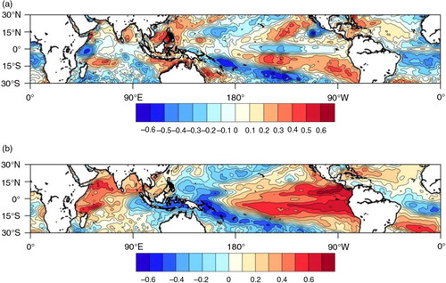
In this work, ENSO state is represented by the Niño3.4 Index, obtained by averaging monthly SST anomalies in the region (5°N–5°S, 120°–170°W) represented in Fig. 1. Our analysis is focused on the data of the satellite era (1980–2012). According to Trenberth's criterion (Trenberth, 1997) nine warm and nine cold events took place in the chosen period. The other basic variable used here is the Warm Water Volume (WWV) Index, obtained by averaging the integrated water volume above the 20°C isotherm along the equator. In the basic model, the atmospheric part of the variability is represented by the SOI. In some other models, the SOI is replaced by the ISV Index, a variable that represents the low-frequency component in the high-frequency surface wind forcing of the equatorial Pacific (see definition in Table 1). In other version, we include instead the Pacific Meridional Mode (PMM) index, obtained from the covariability of the 10 m wind field and the SST in the tropical region between 74°W and 15°E. According to Chiang and Vimont (2004), this pattern plays an important part in the SFM.

Fig. 1 The boxes enclose some regions that are important for the definition of the indexes used in this work. The Niño3.4 Index was produced by averaging the SST in the Niño3.4 region. The South Tropical Zonal Gradient (STZG) and the North Tropical Zonal Gradient (NTZG) Indexes are defined as averages of SST anomalies in the region 6 (region 7) minus those in the region 5 (region 8), respectively.

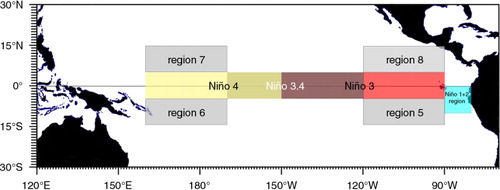
Table 1. Acronyms and specifications of some tropical Climate Indexes and some of the Climate Fields used

Acronym	Index	Definition
SOI	Southern Oscillation Index	Standardised surface level pressure differences between Tahiti and Darwin (Trenberth, 1984).
Niño3.4	Niño3.4	Average anomalies of sea surface temperature in the Niño3.4 region (170°W–120°W, 5°S–5°N, Trenberth, 1997).
WWV-west	Warm Water Volume-west	The integrated warm water volume (WWV) above the 20°C isotherm between 5°N and 5°S, 120°E to 155°W (Meinen and McPhaden, 2000) obtained from Australian Bureau of Meteorology Research Center (BMRC) reanalysis.
WWV-east	Warm Water Volume-east	The integrated warm water volume (WWV) above the 20°C isotherm between 5°N–5°S, 155°W and 80°W (Meinen and McPhaden, 2000) obtained from Australian Bureau of Meteorology Research Center (BMRC) reanalysis.
TSA	Tropical Southern Atlantic	Anomaly of the average of the monthly SST between (0°S–20°S, 10°E–30°W). HadI SST and NOAA OI 1°×1° data sets are used to create this index (Enfield et al., 1999).
PMM	Pacific Meridional Mode SST	The Pacific Meridional Mode is defined via applying maximum co-variance analysis (MCA) to sea surface temperature (SST) and the zonal and meridional components of the 10 m wind field over the time period 1950–2005, from the NCEP/NCAR reanalysis. To define the spatial pattern, data are defined over the region (21°S–32°N, 74°W–15°E), and spatially smoothed (three longitude by two latitude points, (Chiang and Vimont, 2004)).
IOD	Indian Ocean Dipole Mode	The Indian Ocean Dipole is defined as the SST anomaly difference between the western equatorial Indian Ocean (10°S–10°N, 50°E–70°E) and the south eastern equatorial Indian Ocean (10°S–0°, 90°E–110°E), sometimes referred to as Dipole Mode Index (DMI), Saji et al. (1999).
SST	Sea Surface Temperature	Sea Surface Temperature from the ERA-Interim reanalysis (Dee et al., 2011). 0.75°×0.75° resolution (www.ecmwf.int/en/forecast/datasets).
MTT	Middle Tropospheric Temperature	Middle Tropospheric Temperature data from NOAA's TIROS-N polar orbiting satellites and adjusted for time-dependent biases by the Global Hydrology and Climate Center at the University of Alabama in Huntsville (UAH). 2.5°×2.5° resolution (www.ncdc.noaa.gov/temp-and-precip/msu/index.php).
NTZG	North Tropical Zonal Gradient	SST anomaly differences between (5°–15°N, 160°E–170°W) and (5°–15°N, 120°W–90°W) regions.
STZG	South Tropical Zonal Gradient	SST anomaly differences between (5°–15°S, 160°E–170°W) and (5°–15°S, 120°W–90°W) regions.
ISV	IntraSeasonal Variability	Index of high-frequency surface wind forcing in the western equatorial Pacific bandpass filtered at periods of 30–95 d (5°S–5°N, 120°E–180°E, McPhaden et al., 2006).

Recent studies have highlighted the importance of the tropical zonal SST gradients in the linkage with the extratropics (Yu and Kim, 2013) and in the response to the anthropogenic forcing (Karnauskas et al., 2009). Therefore, we will consider also in our study two other indexes that take into account the zonal SST gradient. The NTZG Index, obtained as the difference between the averaged SST anomalies in region 7 and those in region 8 of Fig. 1, represents the North Tropical Zonal Gradient. The STZG Index, computed as the difference between the averaged SST anomalies in region 6 minus those in region 5 of the same figure, represents the South Tropical Zonal Gradient. Alternatively, we consider the effects that the Gulf of Guinea warm events might have on the tropical Walker circulation and introduce the Tropical South Atlantic (TSA) Index as the third variable. In some cases, the indexes were taken from the US National Oceanic and Atmospheric Administration (NOAA) webpage. In other words, we obtained them from the corresponding data fields, according to the procedures described in Table 1.

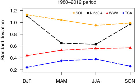
In every case, the variables used in this study are seasonal anomalies. That is, seasonal averages of each variable are built, and from this the seasonal mean was estimated. The seasonal values are obtained as an average of the December, January and February values for boreal winter, of March, April and May for boreal spring, of June, July and August (JJA) for boreal summer and of September, October and November for boreal autumn. Seasonal anomalies were obtained by removing the seasonal mean from the seasonal averages. In Fig. 2, we have represented the seasonal dependence of the standard deviation of some of the indexes.

Fig. 2 Seasonal standard deviation values of the Niño3.4 Index (black squares), the SOI (orange circles), the WWV Index (red triangles) and the TSA Index (blue diamonds).

In the second part of this work, we sought to remove the persistence barrier in summer and autumn and look for fields that include known extratropical precursors of the Niño3.4 Index. An obvious choice was the global SST field obtained from ERA-INTERIM reanalysis (Dee et al., 2011) on a spatial grid of 0.75°×0.75°. In the election of the variables that characterise the atmospheric precursors, we considered the results of previous researches that highlight the part that the atmospheric variability from the surface up to mid-troposphere plays in the SFM. After some preliminary studies, we have selected the global Middle Tropospheric Temperature (MTT) field (Mears and Wentz, 2009), at a resolution of 2.5°×2.5°. From this last field, we have obtained some regional variables to represent the state of the atmosphere in different domains, such as the NP, the Southern Pacific or RB region and the Global Southern Extratropics (GSE) domain. Each of these fields has been expanded in terms of its Empirical Orthogonal Functions (EOF).

3. Models

3.1. The seasonal approach

We examine the behaviour of the 20 first Principal Components (PC) considering: (1) the percent of variance explained, (2) the significance of the lag correlation coefficients between each PC and the Niño3.4 Index at a lead near to those forecast, and (3) if there are signs of a feedback relationship in that lag correlation coefficient. This last condition is important and establishes a difference between this study and other predictability studies mentioned above. As an example, in Fig. 3 the statistically significant negative (positive) correlation coefficient between the Niño3.4 Index and the third PC of the MTT field in the GSE domain at negative (positive) lags supports the existence of a feedback between the variabilities represented by those indexes. For the sake of comparison, we have also represented in the same figure the correlation between the Niño3.4 Index and the WWV Index.

Fig. 3 The lead–lag correlation coefficients between the Niño3.4 Index and the WWV Index (long dashed line), and between the former index and the third PC (short dashed line) of the MTT anomalies in the GSE region are depicted in (a) (summer) and (b) (autumn). In the background, we have represented the autocorrelation functions of the Niño3.4 Index (black solid line). The red dashed lines represent the statistical significance threshold at 95% confidence level.

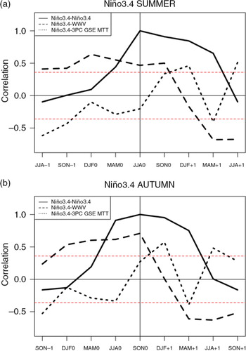
In Fig. 3, we can appreciate the dependence of the lead–lag correlation coefficients on the target season of the Niño3.4 Index. This seasonal dependence can be captured by introducing the seasonal dependence into the parameters of the stochastic model.

3.2. The feedback model

Sometimes we find physical systems, whose variables can be described either as slow or as fast, because they evolve according to two well-separated characteristic time scales. Let the state of the system at a given season s be characterised by a small number of n ‘slow’ variables, including the Niño3.4 Index, that we collect into a (n×1) vector y ^s . If there is a considerable number m of observations of y ^s at different times that can be collected in a Y ^s (n×m) matrix, the time evolution of y ^s can be described by the set of equations (Hasselmann, 1988)1 $\frac{\mathrm{d}{\mathbf{y}}^{\mathbf{s}}}{\mathrm{d}t}={\mathbf{A}}^{\mathbf{s}}{\mathbf{y}}^{\mathbf{s}}+{\mathbf{n}}^{\mathbf{s}}\left(\text{t}\right)$1

where A ^s is a (n×n) dynamical or feedback matrix that represents the effects that the state of the variables at time t has on the future state at time t+Δt (where Δt is the forecast lead) and the n ^s are the residuals of the model identification (ideally white). The A ^s matrix is commonly identified from the data covariance matrices at lag Δt, C ^{1 s} and at lag 0, C ^{0 s} : A ^s =( C ^{1 s} − C ^{0 s} )*( C ^{0 s} )⁻¹. Its eigenvectors yield a new spatial basis U ^s whose time evolution is an exponential function of the eigenvalues ${\lambda }_i^s$ 2 ${\mathbf{A}}^{\mathbf{s}}{\mathbf{U}}^{\mathbf{s}}={\mathbf{\wedge }}^{\mathbf{s}}{\mathbf{U}}^{\mathbf{s}}$2

As the A matrix is in general non-symmetric, its eigenvalues can be complex. The complex eigenvalues represent an oscillatory mode. On this ground, the new basis vectors W ^s are usually called the Principal Oscillation Patterns (POP) of the system (Hasselmann, 1988).

If $\mathbf{U}=\left\{{\mathbf{u}}_{\mathbf{i}},i=\mathrm{1...}n\right\}$ 3 $\text{Im}\left({\lambda }_{\text{is}}^{}\right)=0;{\mathbf{w}}_{\text{is}}^{}={\mathbf{u}}_{\text{is}}^{}$3 4 $\text{Im}\left({\lambda }_{\text{i}}^s\right)\ne 0,{\mathbf{w}}_{\text{i}}^s=\text{Re}al\left({\mathbf{u}}_{\text{i}}^s\right);{\mathbf{w}}_{\text{i}+\text{1}}^s=\text{Im}\left({\mathbf{u}}_{\text{i}}^s\right)$4

More details about the seasonal version of the POP analysis used here can be found in the Appendix of OrtízBeviá et al. (2012). Let us collect the n w ^s vectors into a (n×n) matrix W ^s . The temporal evolution of the W ^s vectors, T ^s , is obtained by projecting the Y ^s matrix, onto the W ^s vectors of the new basis.5 ${\mathbf{T}}^{\mathbf{s}}={\left({\mathbf{w}}^s\right)}^{-1}{\mathbf{Y}}^{\mathbf{s}}$5

At this point, two different predictive schemes can be used. In one of these, for each pair of POP, the agreement between the relative evolution of the time coefficients of the i pair of POP, t _i and t _{i +1} , and the one expected from theoretical considerations is tested (von Storch et al., 1995). If there is such an agreement, the POP is considered useful. The predicted value y ^s _p is then modelled as the combination of all the useful pairs of POP that minimise the expression6 $\epsilon ={\Vert y^{\mathbf{s}}\left(t\right)-{\sum }_{\text{i}}{\mathbf{T}}_i^s(t){\mathbf{w}}_i^s\Vert }^2$6

Here this predictive scheme will be labelled as OS, for Optimised Signal.

In the second approach (Penland and Matrosova, 1998), the modelled y ^s is obtained from the solution of the whole inhomogeneous equation (1). If G ^s (τ) is the Green function, given by7 ${\mathbf{G}}^s\left(\tau \right)=\sum _{k=1}^n{e}^{{\mu }_k^s\Delta \tau }{\left({\mathbf{W}}^s\right)}^{-1}$7

Moreover, if Q ^s is the noise covariance matrix at a season s given by8 $Q^s=<{\text{n}}^{{\text{s}}^{\prime }}{\text{n}}^{\text{s}}>$8

We can express the noise as a function of its eigenvalues ${\pi }_j^s$ and its eingenvectors ${\psi }_j^s$ 9 ${\mathbf{n}}^s\left(t\right)=\sum _{j=1}^n{\mathbf{\psi }}_j^s{\mathbf{\pi }}_j^s{\mathbf{R}}_j^s$9

while the ${\mathbf{R}}_j^s\left(t\right)$ coefficients must satisfy the white noise requirements10 $<R_j^s\left(t\right)R_j^s\left(t^{\prime }\right)>\delta \left(t-t^{\prime }\right)$10

and the solution of the inhomogenous equation is given by11 ${\mathbf{y}}^s\left(t+\Delta t\right)={\mathbf{G}}^{\text{s}}\left(\Delta t\right)y^s\left(t\right)+{\mathbf{G}}^s\left(t+\Delta t\right){\int }_t^{t+\Delta t}{\mathbf{G}}^{s-1}\left(\tau \right)\left(\sum _{j=1}^n{\psi }_j^s{\pi }_j^s{\mathbf{R}}_j^s\left(\tau \right)d\tau \right)$11

In this way, some characteristics of the noise are introduced into the hindcast. This predictive scheme will be referred to here as FSM for Full Stochastic Mode.

As we can see in the complete solution of eq. (1), the part of the noise is crucial in maintaining the oscillation, the solution of the homogeneous equation having the form of a damped oscillation. Some insight into the nature of the noise that is contributing to maintain the oscillations can be gained through the ‘maximum growth structure’ as defined in Penland and Sardeshmukh (1995). This can be identified from an S matrix defined as12 $\mathbf{S}={\left(y^s\left(0\right)\right)}^{\prime }{\left({\mathbf{G}}^s\left(\tau \right)\right)}^{\prime }{\mathbf{G}}^s\left(\tau \right){\mathbf{y}}^s\left(0\right)$12

The S matrix is symmetric: its eingenvalues and eigenvectors are real. The ‘maximum growth structure’, the forcing that is exciting the optimal structure, is basically the S matrix eigenvector corresponding to the largest eigenvalue.

We measure the performance of this predictive scheme by the correlation skill, that is the correlation coefficient between the observed seasonal Nino3.4 Index and the Index simulated with the POP time coefficient.13 $r=\frac{y_0^s*y_m^s}{\left[{\sigma }^s\left(y_0^s\right){\sigma }^s\left(y_m^s\right)\right]}$13

where ${\mathbf{y}}_0^s$ is the (1×m) centred vector of the observations of the Niño3.4 Index, and ${\mathbf{y}}_m^s$ is the transposed of the (1×m) vector of the Niño3.4 Index predicted by the model. ${\sigma }^s\left({\mathbf{y}}_0^s\right)$ and are the respective standard deviations. The correlation coefficients are tested for statistical significance assuming that the variables have a Gaussian distribution (Fisher, 1921). The chosen significance level is the usual 95% confidence level. By analogy with the synoptic forecasts case, skill values exceeding the r _u =0.60 threshold value are considered useful (Hollingsworth et al., 1980).

The predictive performance is measured also by the Root Mean Square Error (RMSE), defined as:14 $RMSE={\left(\mid y_o^s\mid -{\mid y_m^s\mid }^{\prime }\mid y_o^s\mid -{\mid y_m^s\mid }^{\prime }\right)}^{1/2}$14

The RMSE values are compared with the statistical significance threshold computed by assuming the variables’ Gaussianity (Wilks, 1962). They are also tested against an useful threshold derived by using an ${\mathbf{y}}_m^s=r_u{\mathbf{y}}_o^s$, where r _u is the useful threshold according to Hollingsworth et al. (1980). Both parameters were validated by a series of cross-validation experiments. The usual procedure is to leave out from the predictors used in each experiment the observations corresponding to 1 yr at each time. However, here we have found it convenient to omit two consecutive years in each experiment. In this way, the skill values of the hindcasts that have initial and target conditions at the same year and those where initial and target season belong to a different year are directly comparable (the hindcasts contain the same number of years).

3.3. The model setup

We are interested in the simplest model that could represent the anomalous variability in the equatorial Pacific in a way that is both skilful and significant. The recharge–discharge paradigm (Jin, 1997) represents the anomalous state in the region in terms of four variables: the western Pacific thermocline depth anomaly, the eastern Pacific thermocline depth anomaly, the central Pacific zonal wind stress and the eastern Pacific SST anomaly. The CG2003 version reduces the number of variables to three. Finally, Burgers et al. (2005), by relating the central Pacific wind stress and the eastern Pacific thermocline depth anomaly to the eastern Pacific SST anomaly, reduce by two the number of variables of the model. Here we decide the dimensionality of the model according to a parsimony procedure. We will start by hindcasting with a basic model of two variables that represent the anomalous surface and subsurface state of the ocean. We will then hindcast with a model that includes an additional variable that represents the anomalous atmospheric state. We will then compare the hindcasts skill and RMSE, along with the POP performance and physical interpretation. By adding a new variable, we will then proceed to perform a hindcast with a four-variable model, proceed to the same comparison and so on.

4. Analysis

The Niño3.4 Index is the common target of all the predictive schemes developed here. Its seasonal dependence plays an important part in this study. In Fig. 2, we have represented the seasonal dependence of the standard deviation of this index and also of some other indexes used as variables. Note how for the period under study (1980–2012), the spring and summer amount of variability in the Niño3.4 Index are similar.

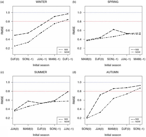
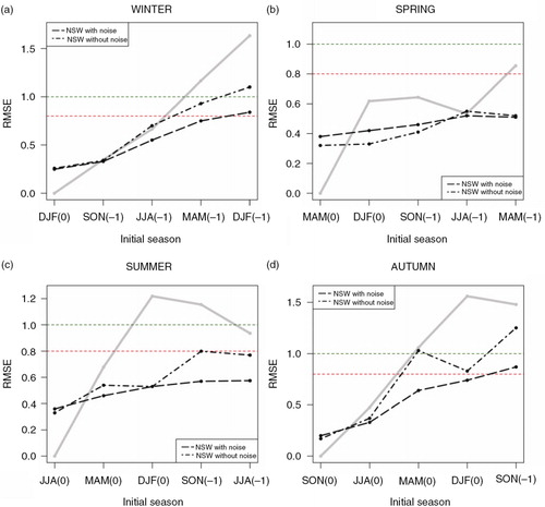
As stated in the methodology, we perform first a series of experiments aimed at determining the minimum dimension that captures the essential evolution of the system. We start with a basic model whose variables are the Niño3.4 Index and the WWV Index (the NW model). From the observations, we identify one dynamical matrix per lag and season, which yields 16 dynamical matrices. We analyse them in terms of their POP, determine the characteristics of its time evolution (frequency and empirical time coefficients) and the corresponding G(τ) operator. We analyse the residuals of the identification of the model in terms of its EOF. We then build two sets of hindcasts for the 1980–2012 period, using both the OS and the FSM predictive schemes and estimate the cross-correlation and the RMSE of those hindcasts. Next we build a basic three-variable model (the NSW model) by adding the SO index to the previous variables and proceed similarly as in the two-variable case. Finally, we test a number of four-variable models built by adding to the NSW model one variable at a time chosen among the indexes that have been pointed out as ENSO precursors, as for instance the ISV Index, the IOD Index or the TSA Index. The relative performance of the two-, three- and four-variable models is compared on the basis of the hindcast cross-correlation and RMSE values and on the consistency of the POP analysis with the POP evolution scheme. The results show that although the NSW model produces cross-correlation skills only slightly over that of the NW model (not shown), lowers the RMSE at most seasons, and considerably for winter and autumn, as shown in Fig. 4. This improvement is not to be found when the cross-correlation and RMSE values produced with the four-variable models are compared with those obtained with the basic NSW model. Additionally, the results of the POP analysis of the three-variable dynamical matrices are always consistent with the POP theoretical scheme, that is, there is always a complex pair and one real eigenvalue. On the contrary, in the case of the two- and four-variable models, for some seasons and lags, the POP analysis exhibits traits that are not consistent with the POP evolution scheme (for instance, all the POP eigenvalues are real). Based on those results, we decided to select the three-variable models as the basic tool of the present predictability studies.

Fig. 4 The RMSE of the NW model hindcast of the Niño3.4 Index (dashed line) and the RMSE of the NSW model hindcast (dot–dashed line) against the hindcast lead, for (a) winter, (b) spring, (c) summer and (d) autumn. The blue straight dashed line represents the statistical significance threshold at 95% confidence level. The red dashed straight line represents an arbitrary threshold for useful forecast as derived by Hollingsworth et al. (1980).

The model used here as a benchmark includes only equatorial variables: the Niño3.4, the SOI and the WWV Indexes (NSW model). The seasonal correlation coefficient values obtained with this model and the OS predictive scheme and those produced when the model is used with the FSM scheme are represented in Fig. 5. We can appreciate in this figure that the skill values produced with the OS scheme (without noise) decay smoothly in winter and spring, remaining useful for lead times up to three seasons or 1 yr, respectively. However, the summer values remain useful only up to two seasons lead, while in the autumn case the skill is below the threshold at two seasons lead, recovers at three seasons and drops again. Using the more sophisticated FSM prediction scheme (including noise) produces useful winter coefficient values at all leads and useful autumn values at leads up to three seasons, but has not the same success in the summer case. The measure of the forecast skill given by the RMSE (represented in Fig. 6) is better, as expected in a model that is designed to minimise this quantity. The RMSE values obtained with the NSW model and the OS scheme are useful at almost all leads and all seasons with two exceptions. These results can be only partly explained by the correlation and RMSE values produced on the basis of assuming the persistence of the Niño3.4 values, which are represented with a continuous grey line in Figs. 5 and 6, respectively.

Fig. 5 Seasonal cross-correlation of the Niño3.4 Index hindcasts with the NSW model in (a) winter, (b) spring, (c) summer and (d) autumn. The values connected with a dot–dashed line were obtained with the OS predictive scheme and those connected with a dashed line with the FSM scheme. On the background we have depicted the cross-correlation of the hindcast produced assuming the Niño3.4 Index persistence with solid grey line. The blue straight dashed line represents the statistical significance threshold at 95% confidence level. The red dashed straight line represents and arbitrary threshold for useful forecast as proposed by Hollingsworth et al. (1980).

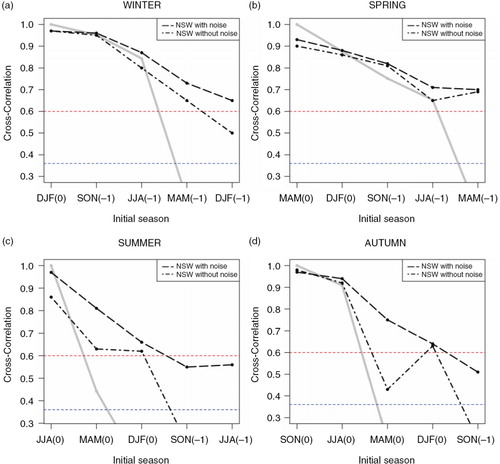
Fig. 6 Seasonal cross-RMSE of the Niño3.4 Index hindcasted with the NSW model in (a) winter, (b) spring, (c) summer and (d) autumn. The values connected with a dot–dashed line were obtained with the OS predictive scheme and those connected with a dashed line with the FSM scheme. On the background we have depicted the cross-RMSE of the hindcast produced assuming the Niño3.4 Index persistence with a solid grey line. The blue and red straight dashed lines represent the same thresholds as in Fig. 4.

We also use other models here that include as third variable, instead of the SOI, either the PMM Index or one of the two zonal indexes (either the NTZG Index or the STZG Index). These models are labelled with NWNTZG or NWSTZG. Another model considers the effect that the SST anomalies in the Tropical Atlantic region might have on the tropical Walker circulation and includes as variable the TSA Index (NWTSA model). In Table 2, we give a description of the tropical models used here with the corresponding acronyms. The most successful of these is the NWTSA whose correlation coefficient and RMSE values are represented in Figs. 7 and 8, respectively. If we compare the correlation coefficients and RMSE values produced by this model with those produced by the NSW model, both used with the OS scheme (represented in Fig. 5), we can appreciate that the NWTSA model brings some improvement of the cross-correlation in winter, and deterioration of the correlation values in summer. However, the correlation values and RMSE produced using the FSM scheme are quite similar. For the sake of completeness (and perhaps to spare other researchers some pain), we have also represented the skill measures of the hindcasts produced by some other three-variable models, when these values scored better than the one produced with the NWTSA run in FSM. The differences in this case are found irrelevant.

Fig. 7 Seasonal cross-correlation of the Niño3.4 Index hindcasted with the NWTSA model in (a) winter, (b) spring, (c) summer and (d) autumn. The values (squares) connected with a dot–dashed line were obtained with the OS predictive scheme and those (filled square) connected with a dashed line with the FSM scheme. As in Fig. 5 the solid grey line represents the cross-correlation obtained assuming persistence. The blue and red straight dashed lines represent the same thresholds as in Fig. 5. Individual symbols (filled circle, triangle, diamond and star) represent the cross-correlation of those models (NWISV, NWPMM, NWNTZG and NWSTZG) that at a given lead score better than the ones obtained at that lead with the NWTSA model.

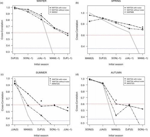
Fig. 8 Seasonal cross-RMSE of the Niño3.4 Index hindcasted with the NWTSA model in (a) winter, (b) spring, (c) summer and (d) autumn. The values (square) connected with a dot–dashed line were obtained with the OS predictive scheme and those (filled square) connected with a dashed line with the FSM scheme. On the background we have depicted with solid grey line, the cross-RMSE of the persistence hindcast. The blue and red straight dashed lines represent the same thresholds as in Fig. 4. Individual symbols (filled circle, triangle, diamond and star) represent the cross-RMSE of those models (NWISV, NWPMM, NWNTZG and NWSTZG) that at a given lead score better than the ones obtained at that lead with the NWTSA model.

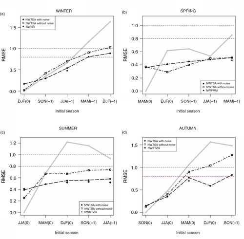
Table 3. Acronyms and specifications of the regions used to build the extratropical predictors

Acronym	Region	Latitude	Longitude
NP	North Pacific	20°N–90°N	140°E–120°W
SP	Southern Pacific	20°S–90°S	160°E–80°W
GSE	Global South Extratropic	20°S–90°S	0°–360°
RB	Ross–Bellingshausen	60°S–90°S	160°E–60°W
SPA	Southern Pacific Antarctic	50°S–90°S	160°E–80°W
SAIA	Southern Atlantic and Indian Antarctic	50°S–90°S	60°W–150°E
SAI	Southern Atlantic and Indian	20°S–90°S	60°W–150°E

Table 2. Acronyms and variables of some tropical models used in this study

Acronym	Model
NW	NIÑO3.4 and WWV Index
NSW	NIÑO3.4, SOI and WWV Index
NWTSA	NIÑO3.4, WWV and TSA Index
NWISV	NIÑO3.4, WWV and ISV Index
NWPMM	NIÑO3.4, WWV and PMM Index
NWNTZG	NIÑO3.4, WWV and NTZG Index
NWSTZG	NIÑO3.4, WWV and STZG Index

There are other cases where the skill differences produced by using one or the other predictive schemes seem important. For instance, such is the case of the summer Niño3.4 hindcasts with the NSW model initialised at the previous spring, as shown in Fig. 5. In this case, we seek to gain some insight into the nature of the noise through the determination of the ‘maximum growth structure’. Among these cases, the quickest growth corresponds to the summer Niño3.4 hindcasts from spring, as already mentioned (the growth exponent is roughly 0). Its ‘maximum growth pattern’ is represented in Fig. 9a. A remarkable trait in this figure is the important anomalies in the South Pacific Convergence Zone region. Another of these cases is the autumn Niño3.4 hindcast from spring initial conditions; its maximum growth pattern, represented in Fig. 9b, has the characteristics of an eastern Pacific warm event and its growth exponent (−0.25) indicates damping.

Fig. 9 (a) The optimal growth structure obtained with NSW model for the summer Niño3.4 Index hindcast initialised from the preceding spring. (b) As in (a) but for the autumn Niño3.4 Index also initialised from spring.

Finally, we will focus on the summer and autumn Niño3.4 Index hindcasts at longer lead times performed with models that include the extratropical variability among their variables. In one case, these were identified from the PCs of the NP region of the global MTT anomalous field, after the inspection of the respective cross-correlation function with the seasonal Niño3.4 Index. The variable selected was the 11th PC of the winter NP MTT field, explaining barely 1% of the variance of the field. In the other case, the variable was obtained with the same procedure, but performed this time from the PCs of the GSE region (see definition in Table 3) of the global MTT anomalous field. Here the third PC (accounting for 13% of the variance of that field) was found optimal. We proceed then to build two new models along the lines of the previous one, the NWNP and the NWGSE. Considering the discussions in the literature relative to the predictive potential of some specific sectors of the Southern Oceans, we have also conducted hindcast experiments with variables extracted from these sectors as the Southern Indian or the Southern Atlantic and Indian (SAI) or the RB Sea or a combination of these (as detailed in Table 3).

The results of these Niño3.4 hindcasts are shown in the Taylor diagrams depicted in Fig. 10. In the summer value hindcasts (Fig. 10a), the modelled standard deviations estimate well the observed one. The skill correlation coefficients of the models whose variables were obtained from the GSE or the Southern Atlantic and Indian Antarctic (SAIA) or SAI regions are above the useful threshold. The RMSE values in turn are well below the corresponding useful threshold. In the case of the autumn hindcasts (Fig. 10b), the models underestimate the observed variability and only the correlation coefficient of that model including the atmospheric variable from the whole GSE domain is above the useful threshold.

Fig. 10 (a) Taylor diagram displaying a statistical comparison (cross-correlation, cross-RMSE and standard deviation) of the hindcasts for the summer Niño3.4 Index, performed with different models initialised in summer. The model variables are the Niño3.4 Index, the WWV Index and another index identified from different extratropical regions: GSE (red), NP (black), SPA (blue), RB (light blue), SAI (green) and SP (brown). (b) As in (a) but for the autumn Niño3.4 Index hindcasts with the models initialised in autumn.

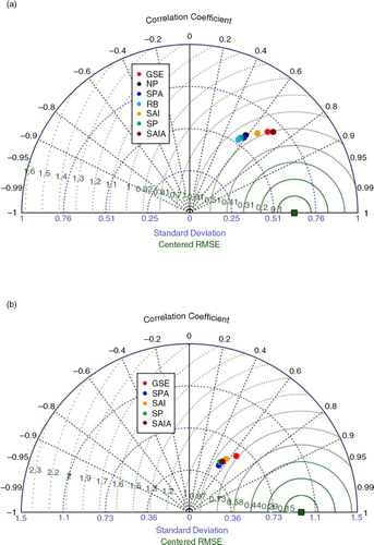
Then, the best hindcast skill produced with the feedback models that incorporate one extratropical predictor improve those produced by the best tropical models by nearly 15%. However, we found that the values obtained by the latter lie inside the confidence intervals of the former, determined at the customary 95% significance level. Therefore, we must acknowledge here that the differences between the skill produced by the model with the extratropical predictor and those of the models that include only tropical variables are not statistically significant.

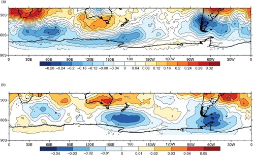
In search of predictability sources, we examine the relevant traits associated with the third PC of MTT, the one included in the NWGSE configuration that scores higher skill at 1-yr lead. Its summer pattern is represented in Fig. 11a and its autumn pattern in Fig. 11b. A relevant feature in Fig. 11a is the wavelike anomalies in the ACC region, more intense in the southern part of South America, and the Southern Indian Ocean. The extension of the MTT anomalies from the South India and South Atlantic Oceans might be explained by a similar WES feedback as suggested by Terray (2011). Furthermore, the pattern here illustrates strong anomalies over the central part of South America that can impact the eastern subtropical South Pacific and from there extend to the equator via a similar feedback (Zhang et al., 2014). In fact, this PC is related to the WAVE3 Mode in the Southern Hemisphere (Yuan and Li, 2008). This is a quasi-stationary pattern (Van Loon and Jenne, 1972) in the southern midlatitudes, a predominant mode in the SLP and v-wind field. A similar mode called the WAVE3N mode is by analogy defined in the Northern Hemisphere. The correlation of the summer or autumn 3rd MTT PC with the corresponding WAVE3 Index is statistically significant, while in summer the correlation with the WAVE3N Index is also significant.

Fig. 11 The figure shows the spatial pattern (EOF) associated with the third PC GSE of the MTT field: (a) for the summer and (b) for the autumn.

5. Concluding remarks

One of the innovative aspects of this study is the use of some linear seasonal statistical model as a tool for the investigation of the Niño3.4 Index longer lead predictability barrier and the solution of the problem. The generality of its formulation made it possible for the model to include variables representing the interactions between the Niño3.4 region and others. This cannot be said of other models, such as CG2003. Here, we use a basic model version to characterise the Niño3.4 ‘predictability barrier’. Moreover, we show that the FSM scheme using this configuration is able to produce hindcast correlations and RMSE similar to the ones scored with the CG2003.

Once the problem is focused on the predictions that target the summer and autumn Niño3.4 conditions, we focus on the analysis of the skill sensitivity to different choices of the variables in the tropical region. Some of these variables such as the TSA and the PMM Indexes are not usually included in a predictive scheme and others such as the STZG or the NTZG Indexes have been defined for the purposes of this study. Finally, we take advantage of the methodology to perform a comparative analysis of the predictive skill gained by including in the model, a particular variable that represent processes and regions identified as longer lead ENSO precursors by previous studies. Among these are the NP region, the ACC region, the RB or the Southern Atlantic and Indian Oceans.

Although some previous work has identified, analysed and even hindcasted with one of these extratropical predictors (Dominiak and Terray, 2005; Boschat et al., 2013) they never went into a comparison of the predictive capabilities of those precursors. Only one very recent study (Dayan et al., 2014) followed a systematic scheme similar to the one used in this one. However, while the focus here is the seasonal predictability barrier, there it is the identification of the best longer lead precursors, and they did not consider feedbacks. The predictive scheme followed is also different: data are severely filtered there while here the seasonal averaging is the only filter applied.

We have found that for the hindcast that target the winter and spring Niño3.4 conditions, it suffices with the equatorial variables to obtain useful skill values. Moreover, including one of the other atmospheric variables has a sizeable impact on the correlation coefficients or RMSE only if the simpler predictive scheme (the OS) is used. That is, when the full stochastic mode (the FSM scheme) is used, the hindcast skill is insensitive to the choice of one or the other atmospheric index as atmospheric variable. Of course, these results are model dependent. However, the comparison with the CG2003 or Barnston et al. (2012) skills supports the validity of our conclusions in the case of the predictions that target the summer months.

The analysis of a great number of sensitivity experiments shows that the higher skill scores correspond to configurations that include variables representing regional MTT anomalies. Predictions from summer initial conditions are the most sensitive to the introduction of extratropical variables. Here again the skill scores obtained by models with atmospheric variables limited to the SAI sector are not very different to those scores of the configurations that include the whole GSE area. This feature is not surprising, because in the spatial pattern of the MTT variable used by these last configurations (third MTT EOF) the main centre of anomalies lies outside of the RB region. This would imply that the SAI region contains most of the skill sources when the target is the summer Niño3.4 condition. However, when the predictand or the predictors are in autumn, the inclusion of the atmospheric anomalous variability in the RB region seems relevant to achieve useful potential skill values, in good agreement with Ballester et al. (2011) analysis. We think that the results here could be of interest not only for predictability studies, but also for coupled model's initialisation.

The results obtained in the last part of this paper show that, when the target are the summer Niño3.4 values and for the longer lead, the introduction of extratropical information leads to skill improvements of more than 15% with respect to the skill obtained with the basic model, which incidentally are not statistically significant. We will address this lack of significance in future research.

Acknowledgements

The authors thank the anonymous reviewers for helpful comments, which improved the presentation of this study significantly. The ERA-Interim SST data used in this paper are available from the European Centre for Medium-Range Weather Forecasts (www.ecmwf.int). Some climate indexes, the NCEP/NCAR Reanalysis datasets were obtained from NOAA (www.cpc.noaa.gov). Some of the figures were produced using the NCAR Command Language (NCL) software package (version 6.1.2). Finally, Miguel Tasambay-Salazar acknowledges the financial support by the SENESCYT (Ecuador).

References

- Anderson B. T . Investigation of a large-scale mode of Ocean–Atmosphere variability and its relationship to Tropical Pacific sea surface temperature anomalies. J. Clim. 2004; 17: 4080–4098. DOI: http://dx.doi.org/10.1175/1520-0442(2004)017 .
- Ballester J , Rodriguez-Arias M. A , Rodo X . A new extratropical tracer describing the role of the Western Pacific in the onset of El Niño: implications for ENSO understanding and forecasting. J. Clim. 2011; 24: 1425–1437. DOI: http://dx.doi.org/10.1175/2010JCLI3619.1 .
- Barnston A. G , Tippett M. K , L'Heureux M. L , Li S , DeWitt D . Skill of real-time seasonal ENSO model predictions during 2002–11: is our capability increasing?. Bull. Am. Meteorol. Soc. 2012; 93: 631–651. DOI: http://dx.doi.org/10.1175/BAMS-D-11-00111.1 .
- Blumenthal M . Predictability of a coupled ocean–atmosphere model. J. Clim. 1991; 4: 766–784. DOI: http://dx.doi.org/10.1175/1520-0442(1991)004 .
- Boschat G , Terray P , Masson S . Extratropical forcing of ENSO. Geophys. Res. Lett. 2013; 40: 1605–1611. DOI: http://dx.doi.org/10.1002/grl.50229 .
- Burgers G , Jin F , Oldenborgh G . The simplest ENSO recharge oscillator. Geophys. Res. Lett. 2005; 32: L13706. DOI: http://dx.doi.org/10.1029/2005GL022951 .
- Chen D. K , Zebiak S. D , Cane M. A , Busalacchi A. J . Initialization and predictability of a coupled ENSO forecast model. Mon. Weather Rev. 1997; 125: 733–788. DOI: http://dx.doi.org/10.1175/1520-0493(1997)125 .
- Chiang J , Vimont D . Analogous Pacific and Atlantic meridional modes of tropical-atmosphere–ocean variability. J. Clim. 2004; 17: 4143–4158. DOI: http://dx.doi.org/10.1175/JCLI4953.1 .
- Clarke A. J , Van Gorder S . Improving El Niño prediction using a spacetime integration of Indo-Pacific winds and equatorial Pacific upper ocean heat content. Geophys. Res. Lett. 2003; 30(7): 1399. DOI: http://dx.doi.org/10.1029/2002GL016673 .
- Dayan H , Vialard J , Izumo T , Lengaigne M . Does sea surface temperature outside the tropical Pacific contribute to enhanced ENSO predictability?. Clim. Dynam. 2014; 43: 1311–1325. DOI: http://dx.doi.org/10.1007/s00382-013-1946-y .
- Dee D. P , Uppala S. M , Simmons A. J , Berrisford P , Poli P , co-authors . The ERA-Interim reanalysis configuration and performance of the data assimilation system. Q. J. Roy. Meteorol. Soc. 2011; 137: 553–597. DOI: http://dx.doi.org/10.1002/qj.828 .
- Dominiak S , Terray P . Improvement of ENSO predictions using a linear regression model with a Southern Indian Ocean sea surface temperature predictor. Geophys. Res. Lett. 2005; 32: L18702. DOI: http://dx.doi.org/10.102972005GL023153 .
- Enfield D. B , Mestas A , Mayer D. S , Cid Serrano L . How ubiquitous is the dipole relationship in tropical Atlantic sea surface temperatures?. J. Geophys. Res. 1999; 104: 7841–7848. DOI: http://dx.doi.org/10.1029/199JC900036 .
- Fisher R. A . On the “Probable Error” of a coefficient of correlation deduced from a small sample. Metron. 1921; 1: 1–32.
- Ham Y. G , Kug J. S , Park J. Y , Jin F. F . Sea surface temperature in the North Tropical Atlantic as a trigger for El Niño-Southern Oscillation events. Nat. Geosci. Lett. 2013; 6: 112–114. DOI: http://dx.doi.org/10.1038/ngeo1686 .
- Hasselmann K . PIPs and POPs: the reduction of complex dynamical systems using Principal Interaction and Oscillation Patterns. J. Geophys. Res. 1988; 93: 11015–11021. DOI: http://dx.doi.org/10.1029/JD093iD09p11015 .
- Hollingsworth A , Arpe K , Tiedke M , Capaldo M , Savijaervi H . The performance of a medium range forecast model in winter: impact of physical parameterization. Mon. Weather Rev. 1980; 108: 1736–1773. DOI: http://dx.doi.org/10.1175/1520-0493(1980)108 .
- Horii T , Ueki I , Hanawa K . Breakdown of ENSO predictors in the 2000s: decadal changes of recharge/discharge-SST phase relation and atmospheric intraseasonal forcing. Geophys. Res. Lett. 2012; 39: L10707. DOI: http://dx.doi.org/10.1029/2012Gl051740 .
- Izumo T , Vialard J , Lengaigne M , Montegut C. B , Behera S. K , co-authors . Influence of the state of the Indian Ocean Dipole on the following year's El Niño. Nat. Geosci. 2010; 3: 168–172. DOI: http://dx.doi.org/10.1038/ngeo760 .
- Jansen M. F , Dommenget D , Keenlyside N . Tropical atmosphere–ocean interactions in a conceptual framework. J. Clim. 2009; 22: 550–567. DOI: http://dx.doi.org/10.1175/2008JCLI.2243.1 .
- Jin E. K , Kinter J. L . Characteristics of tropical Pacific SST predictability in coupled GCM forecast using the NCEP CFS. Clim. Dynam. 2009; 82: 675–691. DOI: http://dx.doi.org/10.1007/s00382-008-0418-2 .
- Jin F. F . An equatorial ocean recharge paradigm for ENSO. Part I: conceptual model. J. Atmos. Sci. 1997; 54(7): 811–829. DOI: http://dx.doi.org/10.1175/1520-0469(1997)054 .
- Johnson S , Batisti D , Sarachick E . Empirically derived Markov Models and prediction of Tropical Pacific sea surface temperature anomalies. J. Clim. 2000; 13: 3–17. DOI: http://dx.doi.org/10.1175/1520-0442(2000)013<3327:SIAEDM>2.0.CO;2 .
- Karnauskas K. B , Seager R , Kaplan A , Kushnir Y , Cane M. A . Observed strengthening of the zonal sea surface temperature gradient across the Equatorial Pacific Ocean. J. Clim. 2009; 22: 4316–4321. DOI: http://dx.doi.org/10.1175/2009JCLI2936.1 .
- Keenlyside N. S , Ding H , Latif M . Potential of equatorial atlantic variability to enhance El Niño Predictions. Geophys. Res. Lett. 2013; 40: 2278–2289. DOI: http://dx.doi.org/10.1002/grl.50362 .
- Kirtman B , Anderson A , Kang I.-S , Scaife A , Smith D , Asnar G. R , Hurrell J. W . Prediction from weeks to decades. Climate Science for serving Society. 2013; Berlin: Springer. 205–235.
- Kirtman B. P . Oceanic Rossby wave dynamics and the ENSO period in a coupled model. J. Clim. 1997; 10: 1690–1705. DOI: http://dx.doi.org/10.1175/1520-0442(1997)010 .
- Luo J. J , Zhang R , Swadhin K , Behera Y , Masumoto F. F , co-authors . Interaction between El Niño and extreme Indian Ocean Dipole. J. Clim. 2010; 23: 726–742. DOI: http://dx.doi.org/10.1175/2009JCLI3104.1 .
- McPhaden M. J , Zhang X , Hendon H. H , Wheeler M. C . Large scale dynamics and MJO forcing of ENSO variability. Geophys. Res. Lett. 2006; 13: L16702. DOI: http://dx.doi.org/10.1029/2006GL026786 .
- Mears C. A , Wentz F. J . Construction of the remote sensing systems v3.2 atmospheric temperature records from the MSV and AMSV microwave sounders. J. Atmos. Ocean. Technol. 2009; 26: 1040–1056. DOI: http://dx.doi.org/10.1175/2008JTECHA1176.1 .
- Meinen C. S , McPhaden M. J . Observations of Warm Water Volume changes in the Equatorial Pacific and their relationship to EL Niño and la Niña. J. Clim. 2000; 13: 3551–3559. DOI: http://dx.doi.org/10.1175/1520-0442(2000)013<3551:OOWWVC>2.0.CO;2 .
- Miller A. J , Cayan D , Barnett T. P , Graham N. E , Oberhuber J. M . The 1976–1977 climate shift of the Pacific ocean. Oceanography. 1994; 7: 21–26. DOI: http://dx.doi.org/10.5670/oceanog.1994.11 .
- Moore A. M , Kleeman R . The dynamics of error growth and predictability in a coupled model of ENSO. Q. J. Roy. Meteorol. Soc. 1996; 122: 1405–1446. DOI: http://dx.doi.org/10.1002/qj.49712253409 .
- OrtízBeviá M. J , Alvarez-García F. J , Ruiz de Elvira A. M , Liguori G . The western Mediterranean summer variability and its feedbacks. Clim. Dynam. 2012; 39: 3103–3120. DOI: http://dx.doi.org/10.1007/s00382-012-1400-s .
- Penland C , Magorian M . Prediction of Niño3 sea surface temperature anomalies using linear inverse modeling. J. Clim. 1993; 6: 1067–1176. DOI: http://dx.doi.org/10.1175/1520-0442(1993)006 .
- Penland C , Matrosova L . Prediction of tropical Atlantic sea surface temperatures using linear inverse modeling. J. Clim. 1998; 11: 483–496. DOI: http://dx.doi.org/10.1175/1520-0442(1998)011 .
- Penland C , Sardeshmukh P. D . The optimal growth of tropical sea surface anomalies. J. Clim. 1995; 8: 1999–2024. DOI: http://dx.doi.org/10.1175/1520-0442(1995)018 .
- Rodriguez-Fonseca B , Polo I , García-Serrano J , Losada T , Mohino E , co-authors . Are Atlantic Niños enhancing Pacific ENSO events in recent decades?. Geophys. Res. Lett. 2009; 36: L20705. DOI: http://dx.doi.org/10.1029/20099GL040098 .
- Saji N. H , Goswami B. N , Vinachandran P. N , Yamagata T . A dipole mode in the tropical Indian Ocean. Nature. 1999; 401: 360–363.
- Stepanov V. N . Modeling of El Niño events using a simple model. Oceanology. 2009; 3: 310–319. DOI: http://dx.doi.org/10.1134/S0001437009030023 .
- Suarez M. J , Schopf P. S . A delayed action oscillator for ENSO. J. Atmos. Sci. 1988; 45: 3283–3287. DOI: http://dx.doi.org/10.117571520-0469(1988)045 .
- Tasambay-Salazar M , OrtizBeviá M. J , Alvarez-García F , RuizdeElvira A . An estimation of ENSO predictability from its seasonal teleconnections. Theor. Appl. Climatol. 2015. DOI: http://dx.doi.org/10.1007/s00704-0.15-1546-3 .
- Terray P . Southern Hemisphere extra-tropical forcing: a new paradigm for El Niño -Southern Oscillation. Clim. Dynam. 2011; 36: 2171–2199. DOI: http://dx.doi.org/10.1007/500382-GL0-6825-Z .
- Trenberth K. E . Signal versus noise in the Southern Oscillation. Mon. Weather. Rev. 1984; 112: 326, 332. DOI: http://dx.doi.org/10.1175/1520-0493(1984)112 .
- Trenberth K. E . The definition of El Niño. Bull. Am. Meteorol. Soc. 1997; 78: 2771–2777. DOI: http://dx.doi.org/10.1175/1520-0477 .
- Van den Dool H. M , Toth Z . Why do forecasts for ‘near normal’ often fail?. Weather. Forecast. 1991; 6: 76–85. DOI: http://dx.doi.org/10.1175/1520-0434(1991)006 .
- Van Loon H , Jenne D . Zonal harmonic standing waves in the Southern Hemisphere. J. Geophys. Res. 1972; 77: 992–1103. DOI: http://dx.doi.org/10.1029/JC077i006p00992 .
- Venegas S. A , Drinkwater M , Shaffer G . Coupled oscillations in Antarctic sea ice and atmosphere in the South Pacific sector. Geophys. Res. Lett. 2001; 28: 3301–3304. DOI: http://dx.doi.org/10.1029/2001GL12991 .
- Vimont D. J , Alexander M , Fontaine A . Midlatitude excitation of tropical variability in the Pacific: the role of thermodynamic coupling and seasonality. J. Clim. 2009; 22: 518–534. DOI: http://dx.doi.org/10.1175/2008JCLI2220.1 .
- Vimont D. J , Wallace J. M , Battisti D. S . The seasonal footprinting mechanism in the Pacific: implications for ENSO. J. Clim. 2003; 16: 2668–2675. DOI: http://dx.doi.org/10.1175/1520-0442(2003)016 .
- Von Storch H , Burger G , Schnur R , von Storch J.-S . Principal Oscillation Patterns: a review. J. Clim. 1995; 8: 377–400. DOI: http://dx.doi.org/10.1175/1520-0442(1995)008 .
- Wang Y , Lupo A. R , Qin J . A response in the ENSO cycle to an extratropical forcing mechanism during El Niño to La Niña transition. Tellus A. 2013; 65: 22431. DOI: http://dx.doi.org/10.3402/tellusa.V65i0.22431 .
- White W. S , Chen S. C , Allan R. J , Stone R. C . Positive feedback between the Antarctic Circumpolar Wave and the global El Nino- Southern Oscillation wave. J. Geophys. Res. 2002; 107: 29–1–29-17. DOI: http://dx.doi.org/10.1029/200JC00581 .
- Wilks S. S . Mathematical Statistics. 1962; New York: Wiley.
- Wu R , Kirtman B. P , Van Den Dool H . An analysis of ENSO prediction skill in CFS retrospective forecast. J. Clim. 2009; 22: 1801–1817. DOI: http://dx.doi.org/10.1175/2008JCLI2565.1 .
- Yu J. Y , Kim S. T . Identifying the types of major El Niño Events since 1870. Int. J. Climatol. 2013; 33: 2105–2112. DOI: http://dx.doi.org/10.1002/joc.3575 .
- Yuan X , Li C . Climate modes in southern high latitudes and their impacts on Antarctic sea ice. J. Geophys. Res. 2008; 113: C06S91. DOI: http://dx.doi.org/10.1029/2006JC004067 .
- Zhang H , Clement A , Dinezio P . The South Pacific meridional mode: a mechanism for ENSO-like variability. J. Clim. 2014; 27: 769–783. DOI: http://dx.doi.org/10.1175/JCLI-D-13-00082.1 .