Assessing the tangent linear behaviour of common tracer transport schemes and their use in a linearised atmospheric general circulation model

Abstract

The linearity of a selection of common advection schemes is tested and examined with a view to their use in the tangent linear and adjoint versions of an atmospheric general circulation model. The schemes are tested within a simple offline one-dimensional periodic domain as well as using a simplified and complete configuration of the linearised version of NASA's Goddard Earth Observing System version 5 (GEOS-5). All schemes which prevent the development of negative values and preserve the shape of the solution are confirmed to have non-linear behaviour. The piecewise parabolic method (PPM) with certain flux limiters, including that used by default in GEOS-5, is found to support linear growth near the shocks. This property can cause the rapid development of unrealistically large perturbations within the tangent linear and adjoint models. It is shown that these schemes with flux limiters should not be used within the linearised version of a transport scheme. The results from tests using GEOS-5 show that the current default scheme (a version of PPM) is not suitable for the tangent linear and adjoint model, and that using a linear third-order scheme for the linearised model produces better behaviour. Using the third-order scheme for the linearised model improves the correlations between the linear and non-linear perturbation trajectories for cloud liquid water and cloud liquid ice in GEOS-5.

• Meteorology
• dynamics
• adjoint
• data assimilation
• tangent linear model
• advection
• transport

1. Introduction

A number of numerical weather centres develop and maintain a linearised version of their atmospheric general circulation model (AGCM). The linearisation consists of the tangent linear and adjoint models (Errico, 1997), used to describe the forward evolution of perturbations and backward evolution of sensitivities, respectively. The linearised models play a crucial role in four-dimensional variational data assimilation (4DVAR) as well as other data assimilation and modelling applications. The adjoint model can be used to calculate observation impacts (Gelaro et al., 2010) and to estimate the sensitivity to initial conditions (e.g. Doyle et al., 2014).

For the linear (or linearised) model to provide an accurate description of the integration of perturbations, it requires a certain amount of linearity in the underlying model equations. Mechanisms such as cloud formation, turbulence and radiation are inherently non-linear. Normally these kinds of processes are modelled using parameterisations that make inherent use of discontinuous equations. As a result, modelling perturbations of variables affected by these processes using the linearised model requires much care (e.g. Holdaway et al., 2014). The part of the model that represents the resolved scale processes of the atmosphere is known as the dynamical core. The equations used in this part of the model are non-linear, yet the linearisation generally performs well if relatively simple numerical schemes are used (Errico et al., 1993).

Modern numerical methods used to solve the governing equations in a dynamical core are seldom linear. This is particularly evident in advection schemes. Advection (or transport) is a process that often has a linear underlying behaviour and is exactly linear under constant wind forcing. Linear numerical schemes are available for solving advection problems, such as simple upwind and centred finite difference schemes. However, invariably these kinds of schemes have undesirable behaviour in the context of weather and climate prediction. Depending on the choice of scheme it may be overly diffusive, produce phase errors or develop oscillations and negative values. Positivity and monotonicity are important properties for accurate advection of tracers, such as clouds and aerosols. However, Godunov's theorem (Godunov, 1959) states that a linear, monotonic advection scheme cannot be greater than first order accurate. Over the decades since the advent of numerical weather prediction significant effort has gone into developing many types of high-order, shape preserving, non-oscillatory, positive definite advection schemes. Although these schemes are excellent in terms of transporting the atmospheric variables in the full dynamical model, they introduce a degree of non-linearity through the use of non-linear limiters. In fact, Thuburn and Haine (2001) showed that achieving these desirable properties without introducing non-linearity is impossible.

The National Aeronautical and Space Administration (NASA) has recently developed a linearised version of the Goddard Earth Observing System version 5 (GEOS-5) cubed sphere finite volume dynamical core and physics. The full ‘non-linear’ version of GEOS-5 uses non-linear finite volume methods in the horizontal direction, and floating Lagrangian levels, which are periodically remapped back to a reference height, in the vertical direction. During the development of a linearised prognostic cloud scheme, large perturbation growth was identified around the linearisation of the dynamical advection of cloud perturbations. The advection of tracers in GEOS-5 is modelled using the piecewise parabolic method (PPM), which is built upon the second-order van Leer scheme (van Leer, 1977; Colella and Woodward, 1984), with the relaxed monotonicity constraint of Lin (2004) and positive definite constraint of Lin and Rood (1996). In this work, this limiter is referred to as the CWL limiter. Although a degree of non-linearity was expected in this PPM with CWL limiter scheme, large growth of the perturbations was not.

The findings of running the linearised version of GEOS-5 with clouds motivate a more in depth examination of the suitability of this scheme for use in a linearised model. In addition to this, various other schemes are examined to determine if some alternative will be more suitable. For the study, only the tangent linear model is tested. The adjoint and tangent linear models are inherently related, and the coding of a correct adjoint is just confirmed using a dot product test.

The use of non-linear advection schemes for data assimilation has been considered by a number of authors (e.g. Vukicevic et al., 2001; Akella and Navon, 2006). However, these studies did not consider the performance within a full AGCM and did not explicitly examine linearity using the tangent linear model.

The linearity of the transport scheme in GEOS-5 is analysed in three ways. First, a simple off-line one-dimensional (1D) problem in a periodic domain is considered. This allows a comparison of PPM with several other well-known schemes, both linear and non-linear, and simple testing of different kinds of perturbations and resolutions. This also allows for the Jacobian of the scheme to be easily obtained and a linear stability analysis to be performed. This work is discussed in Section 2. The second way in which the schemes are tested is using the linearised version of GEOS-5. It is helpful to test the schemes in a full model that is linear. This is achieved by constructing a passive cloud tracer experiment. In this configuration, clouds are not altered by physics, do not alter the other fields, for example through radiation, and are not subject to remapping of Lagrangian levels. When non-tracer perturbations are set to zero and a linear advection scheme is used, this produces a linear model and useful baseline for testing the non-linear schemes. This is presented in Section 3. The final testing, presented in Section 4, allows perturbations of other variables to be non-zero so the full dynamical core of the linearised version of GEOS-5 is employed. Section 5 offers some concluding remarks.

2. One dimensional model

In this section, the advection equation is linearised in the context of a 1D model. This provides a setting for considering a number of different advection schemes with different underlying functions and perturbations.

For this 1D testing, in addition to the PPM with CWL limiter scheme, the PPM method is tested with a number of other options: the ‘original’ limiter developed by Colella and Woodward (1984) (referred to as the CW limiter), the Colella and Sekora (2008) limiter (referred to as the CS limiter), and a linear version with no limiter. Also tested are first, second and third-order finite-difference schemes, which are linear. The first-order scheme is an upwind scheme, the second-order scheme is Lax-Wendroff (Lax and Wendroff, 1960) and the third-order scheme is an upwind scheme based on a higher-order version of the Lax-Wendroff scheme (Tremback et al., 1987). The third-order scheme can be made non-linear when used with a flux limiter and the universal limiter (Leonard, 1988, 1991) is tested (referred to here as the UL limiter). In addition, a conservative semi-Lagrangian scheme, the Semi-Lagrangian Inherently Conserving and Efficient (SLICE) scheme of Zerroukat et al. (2002), is tested. The version of SLICE employed here uses the parabolic spline method of Zerroukat et al. (2006). The SLICE scheme is tested with and without the Bermejo and Staniforth (1992) limiter (referred to as the BES limiter).

2.1. Model description

The 1D advection equation is given by,1 $\frac{\partial q}{\partial t}+u\frac{\partial q}{\partial x}=0,$1 where q(x,t) is the constituent (or tracer mixing ratio) being advected, u is the wind, or forcing, t is the time and x is the horizontal direction.

Model variables are linearised by splitting into their reference and perturbation parts, for example, q=q ^(r)+q′, where superscript (r) denotes the reference part and superscript ′ denotes the perturbation part. For constant forcing (u′=0), eq. (1) is linear and the linearisation is exact,2 $\frac{\partial q\prime }{\partial t}+u^{(r)}\frac{\partial q\prime }{\partial x}=0.$2 If perturbations u′ were considered then two additional terms, $u\prime \partial q^{(r)}/\partial t$ and $u\prime \partial q\prime /\partial t$ would be present on the right-hand-side. In practice, higher-order products of perturbations would be neglected in the linearisation, making it non-exact. For the work in this section of the article, u′=0 is used. Any non-linearity can only come from the advection scheme.

A semi-discretised version of eq. (2) can be written in vector form,3 $\frac{\partial \mathbf{q}\prime }{\partial t}=\mathbf{M}q\prime ,$3 where M is the operator of the tangent linear model and contains u ^(r) and the derivative operator. The matrix M is often referred to as the Jacobian. The vectors q′ contain q′ at all the discrete locations. In the more complex case, where u′ is considered, the vector on the right-hand-side would also contain u′ terms and M would be non-square.

To solve eq. (1) discretely some form of numerical method must be chosen. If solved with a simple first-order upwind finite difference scheme (for u a positive constant) the solution would be obtained as,4 $q_j^{n+1}=q_j^n-C\left(q_j^n-q_{j-1}^n\right),$4 where superscript n denotes the time step, subscript j denotes the spatial grid point and C=uΔt/Δx is the Courant number. For this simple first-order approximation, M is a diagonal matrix with 1−C on the diagonal and C to the left of the diagonal.

Equation (4) is linear and an identical form would be used to solve eq. (2), replacing, for example, $q_j^{n+1}$ with $\left(q_j^{n+1}\right)\prime$. If this scheme was used to solve advection in an AGCM then the tangent linear model would perform perfectly for that part of the system.

The central issue is that using eq. (4) to solve advection in the non-linear model results in excessive diffusion. Even using higher-order linear schemes can produce unacceptable problems, such as oscillations near discontinuities and negative values. As a result more complex schemes that prevent these issues have been developed, yet all of these approaches invariably and unavoidably introduce non-linearity into the numerical solution through the derivative operator. In this section, the extent of the non-linearity is examined.

2.2. Numerical setup

In this testing, the horizontal domain is periodic on x∈(0,1) and units are dimensionless. The number of grid points is N=64 (the number of grid points is always chosen to be even), and the grid spacing is Δx=1/N. The velocity is constant and set to u=1, and the Courant number is chosen as 0.1 to ensure stability, giving a time step of Δt= 1/640. The model integrates to time 1, that is, for 640 time steps, so that the initial profile returns to its starting point. For this simple case, the exact solution to the equation is equal to the initial conditions.

Three initial profiles are chosen, which can later be perturbed. These are a step function, a sine wave function and a point function. The step function is given by, for grid index j,5 $q_j=\{\begin{array}{cc}1,& \text{if}0.25<x_j<0.75\\ 0,& \text{otherwise}\end{array}.$5 This is discontinuous and will therefore force the use of non-linear limiters in the relevant schemes. The sine wave is chosen as a smooth case that should require limited use of the non-linear components of a scheme and is given by6 $q_j=0.5(1+sin(2\pi x_j)).$6 The point function is a discontinuous function designed to resemble a single small cloud and will also force the use of non-linear limiters in the relevant schemes. The profile is given by7 $q_j=\{\begin{array}{cc}1,& \text{if}j=N/2\\ 0,& \text{otherwise}\end{array}.$7

Three separate runs are required to test each numerical scheme for a given perturbation. First, an integration of the full (possibly non-linear) advection scheme to obtain m(q); second, an integration where the perturbations are added to the inputs, to obtain m(q+δ q), where δ q=q′; third, an integration of the tangent linear model to obtain M δ q. The difference m(q+δ q)−m(q) is referred to as the non-linear perturbation trajectory; for clarity, this expression is used even when the schemes in use are linear. The M δ q term is the linear perturbation trajectory, or tangent linear result. Here, lower case m is the non-linear model, and δ q is some perturbation.

The tangent linear versions of each non-linear scheme can be quickly obtained using the Tapenade auto differentiation tool (Hascoët and Pascual, 2013). The tool effectively takes Fortran subroutines and linearises the algorithm in a line-by-line sense. A new subroutine is produced that evolves the perturbations whilst also updating the model trajectory where required. The tool can also be used to provide adjoint versions of the algorithms.

The performance of each scheme is determined by three metrics. First, by comparing the tangent linear result with the true solution using the root mean squared, or ${}^2$, error. In this simple environment, the true solution is equivalent to the initial conditions. Second, the performance of the tangent linear model can be straightforwardly measured by computing what is referred to here as the gradient test,8 $\underset{\delta q_j\to 0}{lim}\frac{y_j^p-y_j^f}{y_j^{tl}}=1,$8 where $y_j^p$, $y_j^f$ and $y_j^{tl}$ indicate vectors m(q+δ q), m(q) and M δ q evaluated at the grid point with index j. Note: the field can be perturbed at multiple grid points simultaneously or at single grid points. The equation states that for a small enough perturbation, the tangent linear model will accurately approximate the change that the perturbation would undergo in the non-linear model. In practice, correlations between the non-linear and linear perturbation trajectories are computed. This avoids the need to account for grid points where perturbations are zero. When a linear scheme is used to solve the linear advection problem, eq. (8) reduces to being exactly one and for all perturbation sizes. For linear schemes, the non-linear and linear perturbation trajectories will be identical, to the numerical precision of the calculation.

The final metric is the normalised ${}^2$ error of the gradient test. For each scheme, the non-linear perturbation trajectory, m(q+δ q)−m(q), is compared with the result from the tangent linear model, M δ q at each grid point. For a linear scheme, the difference between them is zero (to machine precision).

The use of limiters in the non-linear schemes is controlled by the underlying advected field, q. The ability of a given non-linear scheme to model the advection of a perturbation will depend on the structure of the perturbation δ q, the smoothness of the underlying advected field and the interaction between any discontinuities in the perturbation and discontinuities in the underlying field.

2.3. Results

Before analysing the behaviour of the tangent linear versions of the schemes, the behaviour of the full schemes is examined. Any scheme used for the linearised model must be chosen in the context of how it performs in general. The schemes being considered are summarised in Table 1.

Table 1. List of schemes used in 1D case study

Scheme type	Non-linear limiter	Limiter acronym
First-order FD	None
Second-order Lax-Wendroff	None
Third-order FD	None
PPM	None
PPM	Colella and Woodward (1984)	CW
PPM	Colella and Sekora (2008)	CS
PPM	Colella and Woodward (1984) + Lin (2004)	CWL
Third-order FD	Leonard (1991) (universal)	UL
SLICE	None
SLICE	Bermejo and Staniforth (1992)	BES

From left to right the columns show the type of scheme, the limiter used (if any) and the acronym used for the limiter.

Figure 1 shows the advection, once around the domain, for the step function (top row), the sine function (middle row) and the point function (bottom row). The figure shows the advection of the full field q with a selection of schemes: the first-order finite-difference scheme, the third-order finite-difference scheme, PPM with no limiter and PPM with the CWL limiter.

Fig. 1 Advection, once around the domain, of the step function (top row), the sine function (middle row) and the point function (bottom row). The first-order finite difference scheme is shown in panels (a, e and i). The third-order finite difference scheme is shown in panels (b, f and j). The unlimited PPM scheme is shown in (c, g and k). The PPM with CWL limiter is shown in (d, h and l). The grey curve shows the exact solution (equal to the initial conditions for this simple case). The black curves show the result when using the different schemes.

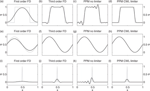
The step function demonstrates how the schemes perform for discontinuous data. It is clear that the scheme that preserves the shape of the profile most accurately is the PPM scheme with CWL limiter. The other three schemes all suffer from some degree of issue. The first-order finite difference scheme is overly diffusive, although remains positive. The third-order scheme and unlimited PPM scheme are not diffusive enough, and both develop oscillations around the discontinuities, resulting in regions with negative values. Comparing with the third-order finite difference scheme, the unlimited PPM scheme has a smaller root mean squared error (RMSE) but larger mean error and maximum error when compared to the true solution.

All of the other schemes were examined for these initial profiles. For the step function, all of the other limited schemes behave very similarly to the PPM with CWL limiter (not shown). The SLICE scheme without the BES limiter behaves similarly to the unlimited PPM scheme. The SLICE scheme that does use the BES limiter performs similarly to the PPM schemes with limiters. However, the SLICE scheme tends to have phase error slightly upwind of the peak.

The sine function tests the schemes ability to advect smooth data. Again, the first-order scheme is overly diffusive. The higher-order linear schemes perform well for the smooth data. The non-linear schemes produce results similar to the linear schemes, except that the peak and trough of the sine wave has been slightly damped. This is due to the non-linear limiters switching on at the peaks.

All of the schemes tested damp the amplitude of the point function as it is advected. Again, the first-order scheme is highly diffusive, reducing the maximum of the point significantly. The unlimited PPM scheme and the second-order finite difference scheme (not shown) have large oscillations just upwind of the discontinuity. The third-order scheme appears similar to the PPM with CWL limiter, except that the third-order scheme has produced oscillations and negative values.

There are an unlimited number of ways to perturb the three initial conditions considered here. Each potential choice of perturbation can result in different behaviour, depending on the scheme and the structure of the initial conditions. To highlight a range of behaviour, a point perturbation is considered. The perturbation field has the same structure as the point function, with an infinitesimally small amplitude. To avoid negative values, a positive perturbation is chosen.9 $q_j\prime =\{\begin{array}{cc}1\times {10}^{-4},& \text{if}j=N/2\\ 0,& \text{otherwise}\end{array}.$9  By testing the three initial conditions with the point perturbation, three specific situations arise: one where discontinuities in the actual field are inconsistent with discontinuities in the perturbation (step function); one where there are no discontinuities in the actual field (sine wave); and one where discontinuities in the perturbation are consistent with discontinuities in the actual field (point function).

2.3.1. Finite difference schemes.

The first, second and third-order finite difference schemes that have no limiter are all linear. For these schemes, since they are linear, the evolution of perturbations performs identically to the evolution of an equivalently shaped field. The result of the gradient test is 1 everywhere, the RMSE is 0, and the normalised ${}^2$ gradient error is 0 (to within numerical precision). These results hold for all perturbation structures and magnitudes.

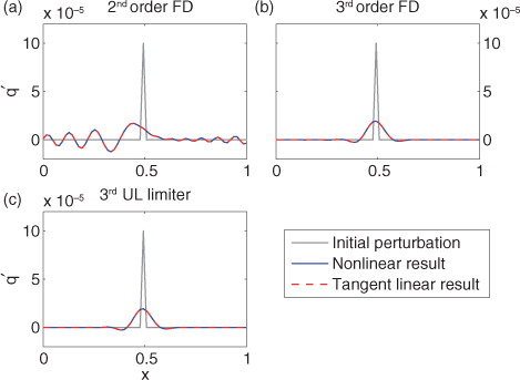
Figure 2 shows the result of advecting the infinitesimal point perturbation when it is applied to the step function initial profile. In this Figure, as well as subsequent figures, the grey curve shows the initial perturbation δ q, the blue curve shows the non-linear perturbation trajectory m(q+δ q)−m(q) and the dashed red curve shows the tangent linear result M δ q. When the scheme is linear, the blue and dashed red curves are equivalent.

Fig. 2 Comparison of the initial perturbation (also the truth solution), the non-linear perturbation trajectory (blue) and the linear perturbation trajectory (red dash) when perturbing the step function initial conditions with a point perturbation.

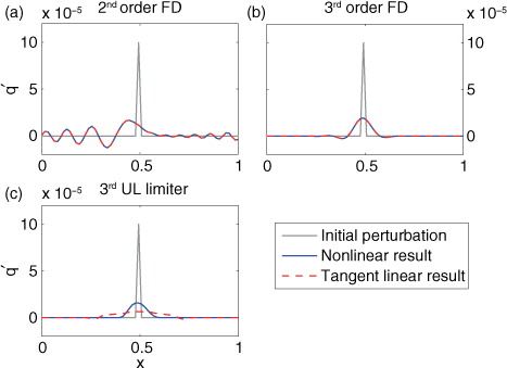
Figure 2a and b shows the result of using the second-order and third-order linear schemes. It is clear that the tangent linear versions behave as expected. However, the issues that affect these kinds of schemes are evident, particularly the second-order scheme which produces significant negative values and oscillations.

Figure 2c shows the result when using the third-order scheme with the UL limiter. Here the blue and dashed red curves differ, showing non-linearity is present. For the step function profile, the non-linear parts of the limited schemes are highly active at the discontinuities. The perturbation field will also be subject to these active parts of the scheme, despite having no structure in these locations. When using the UL limiter the solution is highly diffused and develops negative values. The overall result is worse than if just using the linear third-order scheme.

Figure 3 is similar to Fig. 2 but shows the result when perturbing the sine wave initial conditions. In this situation, the limiters in the non-linear schemes are rarely active since there are no steep gradients or discontinuities to control. There is no change to the behaviour of the linear schemes for the perturbation, plot (a) and (b), compared to the step function since they do not depend on the structure of the underlying profile. From Fig. 3c, it is clear that when the limiter is not often used for the underlying profile the third-order schemes with UL limiter behaves almost exactly as the linear third-order scheme behaves.

Fig. 3 As for Fig. 2 but when perturbing the sine wave initial condition with the point perturbation.

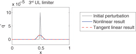
Figure 4 shows the result when perturbing the point function profile with the point function perturbation and using the third-order scheme with UL limiter. In this situation, the non-linear components of the scheme are perfectly aligned to prevent oscillations and negative values that would otherwise occur in the perturbation field. Despite the non-linear components of the schemes being highly active, the result is linear. It is also interesting to note that the limiters work well despite the difference in amplitude between the underlying field and the perturbation. The results for the linear schemes (not shown) are the same as in Figs. 2 and 3.

Fig. 4 As for Fig. 2c but when perturbing the point function initial conditions with the point perturbation.

Table 2 provides the RMSE between the tangent linear perturbation and the exact perturbation, the correlation between the tangent linear perturbation and the non-linear perturbation and the normalised RMSE of non-linear perturbation and the tangent linear perturbation. The linear schemes give a RMSE of zero (to machine precision), and correlations of one. The results are shown for the point perturbation, for each of the three initial conditions. Despite the non-linearity, the third-order scheme with UL limiter performs quite well and has a reasonable correlation for the point perturbation on the step function profile.

Table 2. The root mean square error between the tangent linear perturbation and the exact perturbation (linear schemes are zero), the correlations between the tangent linear perturbation and the non-linear perturbation (linear schemes are one) and the normalised root mean square error of non-linear perturbation and the tangent linear perturbation (linear schemes are zero)

RMSE (${}^2$)	Step function	Sine function	Point function
Third-order UL	1.20×10^−5	1.10×10^−5	1.12×10^−5
PPM CW	3.38×10^−5	1.10×10^−5	1.11×10^−5
PPM CS	1.44×10^−5	1.10×10^−5	1.14×10^−5
PPM CWL	3.20×10^−3	1.10×10^−5	1.12×10^−5
SLICE BES	1.25×10^−3	1.10×10^−5	1.12×10^−5
Correlations	Step function	Sine function	Point function
Third-order UL	0.76	1.00	1.00
PPM CW	0.19	0.99	1.00
PPM CS	0.53	0.93	1.00
PPM CWL	1.41×10^−3	1.00	1.00
SLICE BES	3.64×10^−8	1.00	1.00
${}^2$ Grad test	Step function	Sine function	Point function
Third-order UL	1.0	–	–
PPM CW	1.0	1.10×10^−2	–
PPM CS	0.85	0.40	–
PPM CWL	1.0	5.5×10^−5	–
SLICE BES	12.3	–	–

A dash indicates machine precision.

2.3.2. PPM schemes.

Figure 5 presents the same case shown in Fig. 2 but for the PPM schemes. Figure 5a shows the unlimited PPM scheme which is linear and behaves as expected – the non-linear perturbation trajectory equals the linear perturbation trajectory. Figure 5b shows the PPM with CW limiter scheme. Here the linear and non-linear perturbation trajectories are very different, and the tangent linear version of the scheme produces perturbation values that are twice as large in magnitude as the initial perturbation. Large perturbations occur throughout the region where the step function is non-zero. That the perturbation grows during the integration is due to unstable modes, discussed below.

Fig. 5 As for Fig. 2 but for the PPM type schemes.

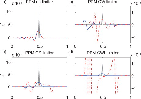
Figure 5c shows the PPM with CS limiter. This scheme is slightly better behaved than the CW limiter in the sense that perturbations do not get as large. At the end time, the maximum magnitude of the perturbation is smaller than at the initial time. However, there is still a large divergence between the non-linear and linear perturbation trajectories, and the largest perturbation structure is seen in locations where it should be zero.

Examining Figure 5d, it is clear that the PPM with CWL limiter has poor tangent linear behaviour. There is very large growth around the location of the discontinuities in the underlying step function. The largest magnitude is around 200 times larger than the initial conditions. The axis on this figure is chosen to show the initial perturbation and non-linear perturbation trajectory. Note that the non-linear perturbation structure does not contain large values away from the perturbation, as seen for some of the other non-linear schemes. This reliable behaviour further supports the case for using this kind of scheme for the non-linear model, even if its tangent linear behaviour is poor. The large growth seen when using the tangent linear version of this scheme is discussed below.

The RMSE and perturbation correlations for the non-linear PPM schemes are included in Table 2. The RMSEs are similar to that seen for the third-order scheme except for the CWL limiter with the step function, which supports large perturbation growth. The low correlations seen for the step function are due to all the limited schemes supporting growing modes in this configuration. It also results from the growth of the non-linear perturbation due to discontinuities in the underlying function. The normalised ${}^2$ of the gradient test highlights how non-linear the PPM schemes with limiters can be. For example, for the point perturbation with the step function, the non-linear perturbation trajectory and the linear perturbation trajectory have an error of the order of 100%. Errors of this magnitude and larger are found for the other non-linear schemes.

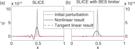
2.3.3. SLICE schemes.

The results for the SLICE scheme with BES limiter are also given in Table 2. Figure 6 shows the result of using the SLICE scheme and the SLICE with BES limiter scheme with the point perturbation applied to the step function. The SLICE scheme is linear and the tangent linear version exactly captures the non-linear perturbation trajectory. The tangent linear version of the SLICE with BES limiter scheme significantly damps the perturbation and any structure that is present is where the left discontinuity of the step function is located. The difference between the two non-linear integrations is reasonable and located where the perturbation structure is expected.

Fig. 6 As for Fig. 2 but for the SLICE schemes.

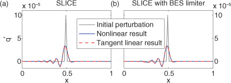
Figure 7 shows the behaviour of the SLICE schemes when the underlying function is the sine wave. For this smooth underlying feature the SLICE scheme does not exceed the bounds of the initial conditions, hence the BES limiter is inactive. The damping does not occur, and oscillations occur in the perturbation field for both schemes.

Fig. 7 As for Fig. 6 but perturbing the sine wave initial conditions.

Examining the tangent linear operator helps to see why the BES limiter causes so much damping. Figure 8 shows the Jacobian for the SLICE scheme and SLICE with BES limiter scheme. From examining the scheme in this way, it is immediately clear that the BES limiter works by masking the scheme away from the discontinuities. The non-zero elements in the SLICE with BES limiter Jacobian are identical to the corresponding elements in the SLICE scheme Jacobian. The limiter prevents negative or too large values occurring, and therefore oscillations, by simply multiplying the input where that value would occur by zero. As the advection continues and the gradient of the discontinuity decreases, more elements will be present. For example at the first time step, when the discontinuity of the step function remains steep, only two rows of the Jacobian contain non-zero values.

Fig. 8 Jacobian of the SLICE scheme and SLICE with BES limiter scheme at time step 292.

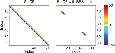
Examining the SLICE schemes in this way demonstrates how the Jacobian can be a useful tool in gaining a physical understanding of how even a non-linear numerical scheme behaves.

2.4. Growing modes

To further understand the observed perturbation growth for certain schemes one can examine individual solutions of the linear system given in eq. (3). Solutions of the equation are sought in the form $\mathbf{q}\prime ~exp\left(\lambda t\right)$, giving $\lambda \mathbf{q}\prime =\mathbf{M}q\prime$. Following standard linear stability theory, the eigenvectors of M give the spatial structure of the solutions (modes) q′ and the eigenvalues give the temporal structure λ. The real part of the eigenvalue gives the growth rate of the corresponding solution, and the imaginary part gives the frequency. If there exist any eigenvalues with real part greater than zero the equation is said to be linearly unstable. For each time step there are N solutions, and they often exist as conjugate pairs.

To compute eigenvalues, the matrix M must first be obtained. Elements M _j,k of the matrix, where j is row and k is column, are obtained by setting inputs qⁿ to either 1 or 0. Consider the expansion of the matrix multiplication that gives perturbations at the new time step,10 $q_j^{n+1}=\sum _{k=1}^N{M}_{j,k}{q}_k^n,\text{for}j=1,\mathrm{...},N.$10 Setting $q_k^n=0$ for all but one k reduces the sum to one term. The equation can then be rearranged to give $M_{j,k}=q_j^{n+1}/q_k^n$. In practice, q is set to 1 at one grid point and zero everywhere else so $M_{j,k}=q_j^{n+1}$. The output of the model is therefore the k ^th column of M, where k is the index at which q is set to 1. The matrix M can be used to perform the advection as a numeric check. At each time step, the eigenvalues are computed and the eigenvalue with the largest real part is recorded.

Table 3 shows a list of all of the non-linear schemes. The middle column shows the average of the eigenvalue with largest real part across all 640 time steps. The column furthest to the right shows the percentage of time steps for which there occurs an eigenvalue with real part greater than zero. To varying degrees of severity all of the non-linear schemes being examined, except the SLICE scheme with BES limiter, are linearly unstable.

Table 3. List of non-linear schemes with the average, over all time steps, of the eigenvalue with largest real part and the percentage of time steps for which an eigenvalue with a positive real part occurs

Scheme	Average max $\Re \left\{\lambda \right\}$	Steps $\Re \left\{\lambda \right\}>0$ (%)
Third-order UL limiter	8.10	61.09
PPM with CW limiter	7.71	100
PPM with CS limiter	48.71	100
PPM with CWL limiter	60.70	100
SLICE BES limiter	0.00	0.00

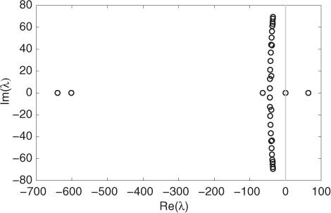
Figure 9 shows the complex plane eigenvalue scatter plot for the third-order scheme with UL limiter at time step 292. Eigenvalues to the left of the grey line correspond to stable modes, those to the right correspond to unstable modes. This figure is representative of other time steps where an eigenvalue with positive real part occurs. It is clear that the majority of the solutions are stable. However, for this time step two solutions are unstable, one significantly so.

Fig. 9 Complex plane scatter plot showing the eigenvalues for the third-order scheme with UL limiter. The eigenvalues are computed for time step 292.

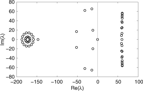
Figure 10 shows the eigenvalues for the PPM scheme with CWL limiter. Here there are a large number of eigenvalues that have very large real part. That perturbations grow when using this scheme is due to the continuous presence of many solutions with large growth rates. Although the limited third-order scheme has unstable solutions they are relatively infrequent and the structures seldom overlap. The other PPM schemes also have unstable solutions at every time. The CW limiter results in smaller growth than the CWL limiter because eigenvalues are generally smaller and fewer unstable solutions exist at each time step. The CS-limited scheme has smaller growth because generally only one or two solutions are unstable at each time step. The eigenvalue spectrum for the PPM scheme with CS limiter is very similar to the third-order scheme with UL limiter.

Fig. 10 As for Fig. 9 but for the PPM scheme with CWL limiter.

2.5. Other perturbations

So far this study has only considered a point perturbation. This was chosen as it highlights a number of different scenarios and is generally the kind of structure that advection schemes struggle with. The same experiments were repeated with a step perturbation and a smooth perturbation.

The step perturbation is a step function narrower than that given in (5).11 $q_j\prime =\{\begin{array}{cc}1\times {10}^{-4},& \text{if}0.35<x_j<0.65\\ 0,& \text{otherwise}\end{array}.$11 For the step perturbation, the results are very similar to those of the point perturbation (not shown). All of the non-linear schemes struggle to capture the perturbation structure and most cause perturbation structure to develop where it should not be present. Unstable modes are a problem whenever the underlying function contains discontinuities. The normalised ${}^2$ norms of the gradient test are of O(1) for the non-linear schemes, when the step perturbation is used with the underlying step and point functions.

A smooth perturbation was obtained by shifting the sine wave profile by a small number of grid points and reducing it to a maximum magnitude of 10⁻⁴. Applying this smooth perturbation to the step and point function profiles resulted in behaviour similar to that of the other perturbations. Even applying the smooth perturbation to the smooth sine wave function resulted in issues, as it could cause steeper gradients to occur in the perturbed non-linear run. The tangent linear versions of the non-linear schemes all perform well but differences between the two non-linear integrations, as seen above, can be large, especially for the PPM with CS limiter scheme. The PPM with CWL scheme gave the smallest RMSE for this case.

The experiments were also repeated for a high resolution case, N=128 grid points. The results were very similar, with problems occurring for the non-linear schemes for the discontinuous underlying profiles (not shown). For the schemes with growing modes perturbations could grow even larger than seen for the lower resolution case.

A further set of experimentation considered different perturbation magnitudes (not shown). No perturbations, smaller or larger than used above, mitigated the issues seen for the non-linear schemes.

2.6. Summary

From examining the simplified 1D case study, it is clear that linearisations of all of the non-linear schemes struggle to represent the tangent linear advection of a perturbation. The schemes only perform well if the underlying profile does not contain any discontinuity or the structure of the perturbation is perfectly orientated with the structure of the underlying field. Both of these situations are somewhat unrealistic, especially for fields like clouds. Furthermore, when the perturbation is not aligned with the underlying structure and discontinuities occur in the underlying field the schemes can behave very poorly. The perturbation structure is seldom captured accurately and most of the linearised schemes support unstable growing modes, which can cause rapid perturbation growth.

This 1D testing helps explain why issues were seen when developing the linearised prognostic cloud scheme in GEOS-5 and motivates the use of a different scheme in the linearised version of GEOS-5. Of the linear schemes examined the third-order finite difference scheme appears to have the best properties. Its use results in minimal negative values, and oscillations are small when compared with other schemes. In practical applications, perturbation fields generally consist of positive and negative values, so small oscillations around zero should not cause issue. The first-order finite difference scheme is far too diffusive. The second order, unlimited PPM scheme and the SLICE scheme all produce large oscillations and can have significant negative values.

3. Passive tracer GEOS-5 model

In this section a simplified version of GEOS-5 is configured, where tracer transport is made passive (i.e. there are no sources or sinks of the constituents). This provides an environment in which to measure the linearity of the advection schemes with realistic underlying fields within the model.

Horizontal advection in GEOS-5 is performed by finite volume methods. The Lin-Rood scheme (Lin and Rood, 1996) is employed to allow the use of 1D operators in solving the 2D problem. Therefore, the advection schemes used to calculate the fluxes in the 1D operators are also 1D (as in Section 2). In all, there are 13 types of advection scheme available in GEOS-5, two of which are in operational use. In the default model, tracers are advected using a limited PPM scheme. The limiter is the CWL limiter described above and used in Section 2. All of the other prognostic variables, including the winds, temperature and pressure, are also solved using a limited PPM scheme. The limiter here is the same as that used for the tracers, except the positive definite constraint is not applied. For testing in this section, the third-order finite difference scheme will also be considered. This scheme is linear, was used in Section 2, and is introduced here as a new option in GEOS-5. The discretisation of this scheme in GEOS-5 is given in the Appendix. The Lagrangian model levels are free to evolve with the flow and would normally be remapped to a Eulerian coordinate at the end of each time step. This remapping involves use of non-linear limiters so is turned off for the tracers. This is not found to result in values outside of the normal range. Note that the vertical remapping could be replaced by a linear method, however the current remapping is an integral part of the full GEOS-5 model (it remaps all prognostic variables, not just tracers), and the aim of this work is to test changes to the advection scheme in the linear model.

The passive cloud tracer with linear advection configuration is obtained by making the following changes. The physics components which either update the clouds or provide a dependency on clouds are adapted in both the non-linear and tangent linear models. The vertical diffusion of tracers and convection and cloud schemes are turned off, and the radiation and aerosols are simplified to assume no cloud cover. In this framework, changes to clouds do not affect other variables and, since vertical remapping of tracers is also disabled, the cloud fields are only altered through the advection.

The testing is constructed similarly to the 1D case study. There are two integrations of the non-linear model and one integration of the tangent linear model. The horizontal resolution of both non-linear and linear models is approximately 55 km. The forecast lengths are 24-hours, the maximum integration length currently used with the linearised version of GEOS-5. The window of the testing is from 0000 UTC on 1 February 2014 to 0000 UTC on 2 February 2014. The first non-linear forecast is obtained by integrating from a realistic set of initial conditions, used to provide operational weather forecasts with GEOS-5. For the second non-linear forecast only the cloud liquid water field q _l is perturbed. The perturbation is applied at the beginning of the window and also used as the initial conditions of the tangent linear model. Since only the cloud field is perturbed, and that perturbation cannot affect other variables, the perturbation is linear. In each non-linear integration the wind fields, temperature, pressure and specific humidity are identical. Their perturbations remain zero throughout the integration of the tangent linear model. As a result much of the linearised dynamical core is redundant and the linearisation becomes exact, provided a linear advection scheme is used.

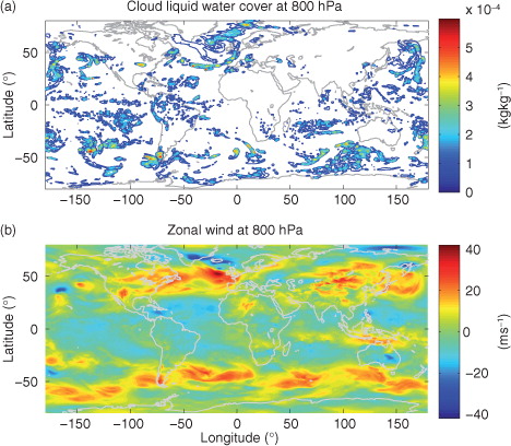
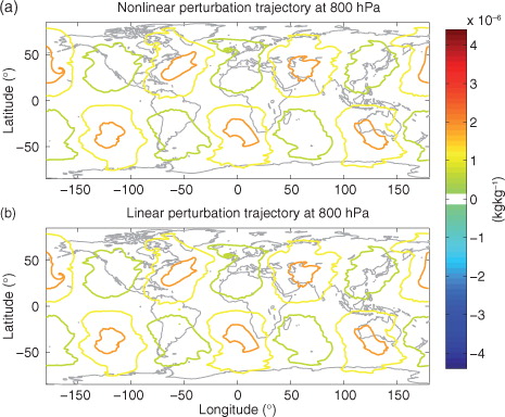
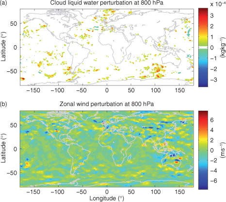
Figure 11 shows the cloud liquid water and zonal wind at the 800 hPa height and at the beginning of the integration window. From the figure it is clear that zonal wind is generally a smoother field than the cloud liquid water. There are many small scale features in the cloud field, and the horizontal gradients are generally larger. The non-linear limiters will play a more active role in the advection of the cloud compared with the advection of the wind.

Fig. 11 Upper panel shows the cloud liquid water field at the 800 hPa height. The lower panel shows the zonal component of wind at 800 hPa.

Several perturbation structures are considered in order to test the schemes. First, the whole cloud liquid water field is positively perturbed by a smooth infinitesimal perturbation, given by,12 $\delta q_l=h_0\left[1+\mid Y_l^m\mid \right].$12 The structure Y is the spherical harmonic function. Here the spherical harmonic of degree l=4 and order m=3 is used. The constant h ₀=10⁻⁷ ensures a perturbation generally much smaller than the cloud field values. All model levels are perturbed by the same quantity. This perturbation structure is chosen so as to smoothly perturb all grid boxes simultaneously, while avoiding having the same structure as the underlying field or creating any negative values. Any growing modes will quickly be identified during the tangent linear integration. A more realistic global perturbation could be obtained but initially the purpose is to perturb all grid boxes without introducing new discontinuities in the tracer field.

First, the CWL limiter is applied to the tracer in both the non-linear and tangent linear models. For the other variables the default option is used in the non-linear model. The choice of advection scheme for the other variables in the linearised model is inconsequential since values are zero. Figure 12 shows the non-linear and linear perturbation trajectories when using the smooth perturbation field and the CWL limiter for the cloud liquid water. The perturbation is shown at the 800 hPa height at the end of the 24-hour integration. On the lower panel, which shows the tangent linear perturbation, it is clear that large spurious perturbation growth is encountered. Many regions are plotted in dark red, showing that very large perturbation quantities are obtained, larger than within the plotting axis. Within the dark red regions are also large negative values of similar magnitude. The largest perturbation magnitude for this model level is 0.56, five orders of magnitude larger than the largest non-linear perturbation.

Fig. 12 Upper panel shows the non-linear perturbation trajectory when using the CWL limiter at the 800 hPa height. The lower panel shows the equivalent tangent linear perturbation. The contour interval is 6×10⁻⁷.

It is interesting to note that problems can occur where cloud cover is relatively low (seen in Fig. 11), for example over the Sahara desert, Eastern Europe, Russia and northern Canada. Problems are often severe where the wind speed is also relatively low. This is perhaps due to smaller changes to the Jacobian from one time step to the next in these regions. This would cause the structures of unstable modes to amalgamate. In many locations, the linearisation of the CWL limiter does produce reasonable results and good agreement with the non-linear perturbation trajectory. In these regions, the limiters are not causing an issue or are inactive.

The non-linear perturbation structure seen in the upper panel of Fig. 12 is not as smooth as one might expect given the results of the 1D case study. The largest perturbation magnitudes have approximately doubled compared with the initial perturbation field, and the field is rather noisy. This results from different use of the limiters in the non-linear forecasts. That such a difference is observed for such a small perturbation further highlights the degree of non-linearity in this scheme.

The use of the CWL limiter without the positive definite constraint in the linearisation results in similarly large linear perturbations when using this same smooth perturbation (not shown).

The linearity of this model configuration is confirmed by repeating the experiment but using a linear advection scheme in both the non-linear and linearised models. Figure 13 shows the perturbation fields at the end of the integration when using the third-order scheme in both non-linear and tangent linear models. The non-linear and linear perturbation trajectories are effectively identical. The smoother more linear behaviour means the structure of the initial conditions is still evident, although deformed by the wind. Perturbations are well behaved, no negative values develop and perturbation magnitudes are similar to the initial conditions. Repeating the experiments with the first-order upwind scheme also produced almost identical results between the non-linear and linear perturbation trajectories, but the perturbation was highly diffused compared to the initial perturbation (not shown).

Fig. 13 As for Fig. 12 but showing the result when using the third-order finite difference scheme in both the non-linear and tangent linear models.

Comparing Fig. 13a with Fig. 12a, it can be seen that the large scale structure of the non-linear perturbation trajectory produced by the third-order scheme is similar to that seen for the PPM with CWL limiter scheme. Where the non-linear model that uses the CWL limiter is well behaved the structures are very similar. Overall the solution using the third-order scheme is less noisy.

This experiment is repeated using the third-order scheme for the tangent linear model but using PPM with CWL limiter for the non-linear trajectories. Results are similar to those seen in Fig. 12b. Further testing with localised perturbations will provide insight into why problems occur for the limited PPM scheme and highlight differences between the limited PPM and third-order schemes in regions where problems do not occur.

A cosine bell and discontinuous cylinder function are used to perturb specific regions of the cloud liquid water. The cosine bell has the form given by Williamson et al. (1992),13 $\delta q_l=\{\begin{array}{cc}\left(h_0/2\right)\left[1+cos\left(\pi r/R\right)\right],& \text{if}r<R\\ 0,& \text{if}r\ge R\end{array}.$13 where14 $r=arccos[sin{\theta }_{c}sin\theta +cos{\theta }_{c}cos\theta cos\left(\lambda -{\lambda }_c\right)].$14

The radius R and centre location (λ _c ,θ _c ) are varied for different tests. A discontinuous cylinder function is similarly given by,15 $\delta q_l=\{\begin{array}{cc}{h}_0,& \text{if}r<R\\ 0,& \text{if}r\ge R\end{array}.$15

Regions in which to make localised perturbations are chosen so as to interact with areas in which the limiters appear to be both highly active and almost inactive. There is a region off the south west coast of Australia where numerous small scale clouds exist. For this perturbation $\left({\lambda }_c,{\theta }_c\right)=\left(124°,-45°\right)$ [converted to radians in eq. (14)]. A second location where steep horizontal gradients occur, but wind speed is smaller, is in the South Pacific, $\left({\lambda }_c,{\theta }_c\right)=\left(-138°,-44.5°\right)$. To see how a perturbation behaves in a region with no cloud cover but strong winds $\left({\lambda }_c,{\theta }_c\right)=\left(100°,50°\right)$ is chosen. To see how a perturbation behaves with no cloud cover and lighter winds $\left({\lambda }_c,{\theta }_c\right)=\left(-10°,20°\right)$ is chosen. All of these locations are far enough apart that all perturbations can be made simultaneously without interacting. Initially R=0.02 is chosen.

Figure 14 shows the non-linear and linear perturbation trajectories when perturbing the initial conditions using the cylinder functions. In this case, the linear third-order scheme is used only in the tangent linear model, and the trajectory and initial conditions come from the non-linear integrations that use the CWL limiter, that is, the third-order scheme is not used in the non-linear model. For the perturbation over the Sahara desert the use of the CWL limiter in the tangent linear model causes large growth to occur. This is a perturbation in a region of relatively low wind speeds. The perturbation over the southern Pacific is in a region of low wind but high cloud cover. One might expect this perturbation to be captured poorly by the tangent linear model with CWL limiter since the limiters are highly active in this region. However, the tangent linear model with CWL limiter, as well as with the third-order scheme, capture this perturbation well. The other two perturbations, are both captured well by both linearised models. For all of the perturbations the third-order scheme captures the overall structure well but by eye appears to be slightly more diffusive. The removal of the positive definite constraint from the CWL limiter makes little difference to the overall perturbation structure (not shown).

Fig. 14 The top panel shows the non-linear perturbation trajectory at the 800 hPa height when perturbing the cloud liquid water using the cylinder functions. The middle panel shows the linear perturbation trajectory when using the CWL limiter. The lowest panel shows the linear perturbation when using the third-order scheme in the tangent linear model. The black curves show the outline of the initial cylinder functions. The contour interval is 2×10⁻⁷.

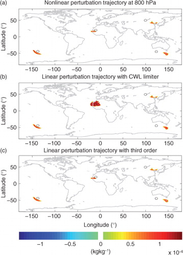
Table 4 shows the RMSEs for the four cylinder perturbations. The calculation assumes the non-linear perturbation trajectory to be the truth. When summing the only points considered are those close to the perturbation and where either the non-linear perturbation trajectory or one of the linear perturbation trajectories are non-zero. For three of the perturbations, the third-order scheme results in a smaller RMSE than when using the PPM with CWL limiter. For the Sahara perturbation the RMSE when using the third-order scheme is two orders of magnitude smaller. For the perturbation over Asia, the PPM scheme has a slightly smaller error but the values are very close. Errors are generally larger in locations where the initial perturbation is more spread out by the wind. In the 1D study, it was seen that the third-order scheme is slightly more diffusive at the peaks whereas the PPM scheme, when unlimited, produces small scale oscillations. That the PPM scheme does not beat the third-order scheme in terms of RMSE here is likely due to these oscillations, not visible on the horizontal plots.

Table 4. Root mean square errors for the cylinder perturbations when using the PPM scheme with CWL limiter and the third-order finite difference scheme

Location	PPM w/CWL	Third-order FD
(−138°, −44.5°)	1.783×10^−7	1.566×10^−7
(−10°, 20°)	1.169×10^−6	2.489×10^−8
(100°, 50°)	1.242×10^−7	1.269×10^−7
(124°, −45°)	8.420×10^−8	6.910×10^−7

The experiment is repeated increasing R to as large as 0.1. As R increases and more grid boxes are perturbed, additional spurious growth is encountered when using the CWL limiter. For example, with R=0.05 some upstream spurious perturbation growth is seen for the perturbation made near Australia (not shown).

All of these experiments are repeated for the smoother cosine bell functions. The results are very similar. Problems still occur when using PPM with CWL limiter in the tangent linear model to the same degree for the perturbation over the Sahara desert. These findings, as well as those of the smooth global perturbation suggest that problems occur due to the underlying wind and cloud field, rather than the shape of the perturbation. Again the third-order scheme captures the structure of the cosine bell functions well, although the peak is slightly diffused.

A higher than third-order scheme could be implemented that would be less diffusive. For example, a fifth-order linear finite difference scheme, or the quasi fifth-order scheme referred to as ORD=6 in Putman and Lin (2007) (which is one of the available options in GEOS-5). Increasing the order of the scheme would increase expense for potentially only localised positive improvement. Efficiency is paramount, especially for adjoint models. In addition to this, near to where the grid is divided between processors, currently there are insufficient halo grid points to support the stencil of schemes higher than third order. The quasi fifth-order scheme of Putman and Lin (2007) uses non-linear changes near the grid edges in GEOS-5. This non-linearity caused spurious perturbation growth when the scheme was tested in the tangent linear model (not shown). As model resolution increases and many processors are used, the benefit of a higher-order scheme would likely reduce.

4. Full GEOS-5 dynamics

In the passive tracer configuration only the cloud perturbations are non-zero. This results in much of the linearised dynamical core being redundant. This simplification is relaxed so that all variables of the tangent linear model are perturbed. These variables are zonal wind u′, meridional wind v′, temperature T′, pressure thickness Δp′, specific humidity q′, cloud liquid water $q_l^{\prime }$ and cloud liquid ice $q_i^{\prime }$. The vertical remapping is also turned on. The simplifications to the model physics remain the same since they introduce significant non-linearity. In addition to this, only realistic perturbations are considered. Focus remains on the newly introduced third-order scheme as the alternative to the default PPM scheme.

The initial conditions for the non-linear model are the same as used above. However, now the initial perturbations are obtained as the difference between a forecast initialised from a background field and a forecast initialised from an analysis field (i.e. the analysis increment). The difference is taken at the end of the 6 hours assimilation window to allow clouds to balance with specific humidity and temperature. All the fields are perturbed by this analysis increment. This provides the kinds of perturbations that the linearised model will encounter in realistic applications.

The initial perturbations for the cloud liquid water and zonal wind fields at 800 hPa are shown in Fig. 15. Comparing with Fig. 11, it is clear that cloud liquid water perturbations occur in regions where the cloud liquid water is located, and that perturbation magnitudes are of a similar order to the field itself. This will test the linearity of the advection schemes for a very realistic situation. For the zonal wind field, the perturbations are generally around an order of magnitude less than the field itself, due to there being less uncertainty than there is for clouds. The same is true for the meridional wind, temperature and pressure thickness.

Fig. 15 The initial cloud liquid water perturbation (top) and zonal wind perturbation (bottom), plotted with a contour interval of 5×10⁻⁵ and 0.7.

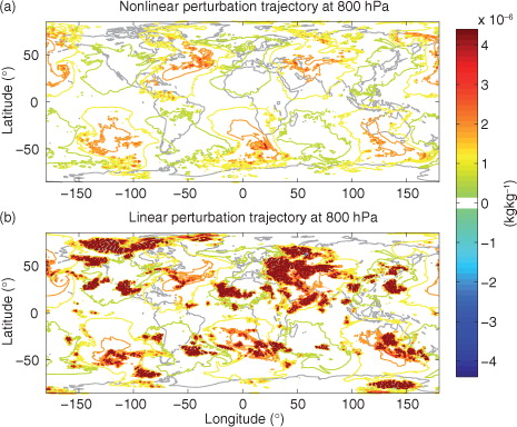
Figure 16a shows the cloud liquid water non-linear perturbation trajectory after 24 hours. Figure 16b shows the cloud liquid water perturbation produced when using the default-limited schemes for all the perturbation variables. Fig. 16c shows the result when the third-order scheme is used for all perturbation variables. Again it is clear that the use of the limiter results in large spurious perturbation growth in multiple locations, although not as severe as seen for the global perturbation. Growing modes are evident over northern Canada. Wind speeds here are relatively small, causing the operator to remain similar from one time step to the next. The third-order scheme results in some diffusion compared with the non-linear perturbation trajectory but generally captures the structures well and has no spurious growth.

Fig. 16 As for Fig. 14 but showing the cloud liquid water perturbation trajectories when using the analysis increment initial condition. The contour interval is 5×10⁻⁵.

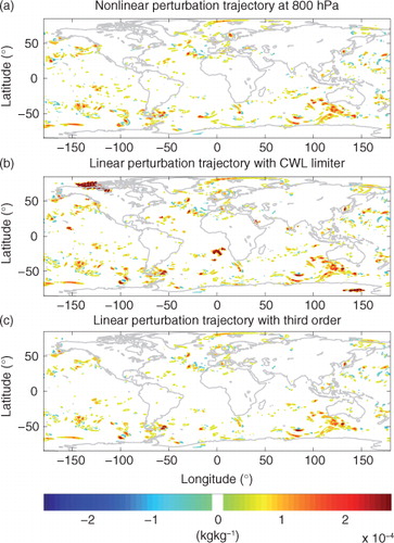
It should be noted that the non-linear scheme can perform well. Consider the region south west of Australia. Here there is a high degree of correlation between the linear and non-linear perturbation trajectories, although a little large in magnitude. The limiters are highly active in this region. This could be a result of the perturbation structure being similar to the underlying cloud structure and the presence of faster wind and so rapidly changing Jacobian.

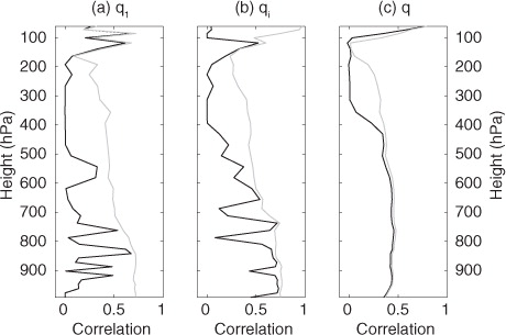
A more quantitative interpretation of the difference between the CWL-limited scheme and the third-order scheme is achieved by computing the correlation with the non-linear perturbation trajectory at each model level. Figure 17 shows the correlations for the cloud liquid water, cloud liquid ice and specific humidity for the 24-hour integration. When the PPM scheme with CWL limiter is used in the tangent linear model, correlations are lower and can even become negative for the clouds. This is as a result of the localised locations where spurious perturbation growth is encountered. When the third-order scheme is used the correlations for cloud liquid water are around 0.7 near the surface, where there is most extensive cloud cover. Cloud liquid ice exists predominantly between 500 and 200 hPa. Here the third-order scheme has much higher correlations than the limited scheme. The specific humidity correlations suggest a better behaviour in the CWL limiter for this field compared to the clouds. The specific humidity field and perturbations are generally quite a bit smoother. This results in fewer instances of the limiter being used and a greater degree of linearity.

Fig. 17 Global correlations between the linear and non-linear perturbation trajectories plotted as a function of pressure. The black curve shows the correlation for the CWL-limited scheme, and the grey curve shows the correlation when using the third-order scheme. The left panel shows the correlations for cloud liquid water, the middle panel for cloud liquid ice and the right panel for specific humidity.

Averaged over all levels where the variables are non-zero the correlations for u′ when using the CWL limiter is 0.718 and 0.719 when using the third-order finite difference scheme. For v′ the correlations are 0.705 and 0.706, for T′ the correlations are 0.695 and 0.696, for q′ the correlations are 0.524 and 0.571, for $q_l^{\prime }$ the correlations are 0.1897 and 0.5258, for $q_i^{\prime }$ the correlations are 0.36 and 0.60, and for Δp′ the correlations are 0.827 and 0.826. With the exception of the pressure, the third-order scheme results in marginally higher correlations for all variables except q _l and q _i , which are significantly larger. Similar results are seen for other days and differently scaled initial conditions (not shown).

For the winds, temperature and pressure the use of the limited PPM schemes is less likely to result in issues due to the relative smoothness of those fields. As can be said for all of these experiments, if the field is so smooth that issues do not occur in the linearised version then the limiter is likely not playing a particularly active role. The scheme being used for the perturbations is therefore just an unlimited PPM scheme, which was demonstrated to result in larger oscillations and negative values in the 1D idealised tests. This is especially true when discontinuities occur in the perturbation field. Even if the underlying field is smooth the perturbations may not be and accuracy could be lost by using the effectively unlimited PPM scheme. This explains why the third-order scheme measures as comparable or better than the non-linear PPM scheme across almost all metrics, except peak amplitude. The third-order scheme is faster, will never produce spurious perturbation growth and is arguably more accurate than an unlimited PPM scheme. As such it should be used for all variables in the linearised version of GEOS-5.

5. Conclusions

The use of several common advection schemes in a linearised version of a numerical weather prediction model has been assessed using a selection of test cases. This work was motivated by finding a suitable advection scheme to use in the linearised version of GEOS-5. Development of the linearised version of GEOS-5 had identified very poor behaviour when linearising the in-situ advection scheme.

A case study that reviewed the advection of a simple 1D profile around a periodic domain was first considered. A simple study such as this provides a straightforward framework for examining several different advection schemes and their linearity. Three different initial underlying profiles, ranging from smooth to highly discontinuous, were considered. To examine the linearity of the schemes, these profiles were perturbed with smooth and discontinuous structures and with structures that exhibited the same structure as the underlying function. Using a variety of metrics, it was shown that all the schemes that employ some degree of non-linearity, through the use of limiters, could have issues when linearised. The limiters are used to prevent oscillations and negative values from developing in the non-linear solution. The determining factors in the behaviour of the linearisation are the shape of the underlying profile and the shape of the perturbation. If any discontinuities occur in the underlying reference field then the limiters will be active. If the shape of the perturbation is identical to the underlying profile then the limiters are well placed to also benefit the advection of the perturbation. If the perturbation has a different shape to the underlying field then the limiters can cause spurious behaviour in the perturbation. When the limiters are inactive the perturbation is advected with the properties of the linear part of the scheme. For example, when the perturbation is a point function but the underlying function is a sine wave function the PPM schemes with limiters perform almost identically to the unlimited PPM scheme.

For the advection of a 1D profile, it is simple to obtain the Jacobian of the scheme and examine the various solutions. For all of the PPM non-linear advection schemes, as well as the third-order scheme with universal limiter, unstable growing modes were identified. The presence of these growing modes leads to the spurious perturbation growth seen for those schemes. The PPM scheme with the relaxed monotonicity constraint of Lin (2004) and positive definite constraint of Lin and Rood (1996) (CWL limiter) had the largest number of linearly unstable modes and the largest growth rates. The only non-linear scheme that is not linearly unstable is the SLICE scheme with Bermejo and Staniforth (1992) limiter (BES limiter). Examining the Jacobian reveals that the BES limiter avoids the development of oscillations and negative values by masking the profile away from any discontinuities. Although this means spurious perturbation growth is avoided, it does mean that when the limiter is active and the perturbation structure is different than the underlying field the scheme completely damps the perturbation.

The linear schemes examined for the 1D advection problem were the first-order, second-order and third-order finite difference schemes, as well as unlimited PPM and SLICE schemes. Of these linear schemes the third-order finite difference scheme had the best overall performance; it maintained most of the structure of the perturbation while developing only minor oscillations and negative values around discontinuities.

In the second half of the article, the use of a different (to the operational model) advection scheme in the linearised version of GEOS-5 was assessed. The performance of the linear third-order finite difference scheme is compared against using the PPM scheme with CWL limiter in the linearised version of GEOS-5. Two configurations of GEOS-5 are considered. First, a passive tracer case, where wind perturbations are equal to zero and small perturbations of the tracer are used. Second, a configuration where wind perturbations are considered and perturbations have realistic structure and magnitude. Throughout these experiments, it is shown that the use of the CWL limiter in the tangent linear model can result in large spurious perturbation growth from linear instability. However, it is also shown that at other points the non-linear scheme can produce good results. Using localised, global and realistic perturbations, it is shown that the non-linear scheme tends to perform poorly when the wind speed is quite small. This is likely a result of a relatively fixed Jacobian and therefore set of linear solutions. From one time step to the next growing solutions amalgamate.

The third-order scheme performs well for all the perturbation structures examined. Although slightly more diffusive than the full non-linear scheme, it results in reasonable structure and magnitudes globally. As a result of this reliable behaviour, the greater degree of efficiency and the demonstrated improvement over an unlimited PPM scheme the third-order scheme will become the scheme used for the advection of perturbations in the linearised version of GEOS-5.

Although it is beneficial to use the same transport scheme in the linear and non-linear models when performing data assimilation (Vukicevic et al., 2001), it is not always possible in practice. The use of non-linear limiters for weather and climate prediction models is considered paramount for obtaining accurate forecasts. Although these limiters work very well in the non-linear model, they are not well suited to being linearised. It is shown here that using a linear third-order scheme for the perturbation advection is an excellent compromise.

6. Acknowledgements

The authors thank John Thuburn, Marek Wlasak and Nigel Wook for providing the 1D SLICE scheme and details of the Met Office approach to linearised advection. The lead author thanks Ron Errico for many useful discussions.

7. Appendix

This appendix describes the discretisation of the third-order advection scheme as implemented in GEOS-5. As GEOS-5 makes use of the Lin-Rood scheme (Lin and Rood, 1996) and the cubed sphere grid, the only changes to the advection scheme are those made to the calculation of the 1D flux. For a tracer q flux-like terms are calculated in the x and y directions and denoted F and G, respectively. If i and j denote the grid indices in the x and y directions, then F, calculated at the boundary of a grid cell, can be discretised asA1 $F_{i-\frac{1}{2},j}=\frac{1}{6}\left(2q_{i,j}+5q_{i-1,j}-q_{i-2,j}\right)-\frac{C_{i-\frac{1}{2},j}}{2}\left(q_{i,j}-q_{i-1,j}\right)\mathrm{\hspace{0.17em} }+\frac{C_{i-\frac{1}{2},j}^2}{6}\left(q_{i,j}-2q_{i-1,j}+q_{i-2,j}\right).$A1

Here C is the Courant number in the x direction evaluated at the boundary of the grid cell. Note that for negative velocity, the flux-like term becomesA2 $F_{i-\frac{1}{2},j}=\frac{1}{6}\left(2q_{i-1,j}+5q_{i,j}-q_{i+1,j}\right)-\frac{C_{i-\frac{1}{2},j}}{2}\left(q_{i,j}-q_{i-1,j}\right)+\frac{C_{i-\frac{1}{2},j}^2}{6}\left(q_{i+1,j}-2q_{i,j}+q_{i-1,j}\right).$A2

The discretisation can be repeated with i and j switched to calculate G.

References

- Akella S. , Navon I. M . A comparative study of the performance of high resolution advection schemes in the context of data assimilation. Int. J. Numer. Methods Fluids. 2006; 51(7): 719–748.
- Bermejo R. , Staniforth A . The conversion of semi-Lagrangian advection schemes to quasi-monotone schemes. Q. J. Roy. Meteorol. Soc. 1992; 120: 2622–2632.
- Colella P. , Sekora M. D . A limiter for PPM that preserves accuracy at smooth extrema. J. Comput. Phys. 2008; 227: 7069–7076.
- Colella P. , Woodward P. R . The piecewise parabolic method (PPM) for gas-dynamical simulations. J. Comput. Phys. 1984; 54: 174–201.
- Doyle J. , Amerault C. , Reynolds C. , Reinecke P. A . Initial condition sensitivity and predictability of a severe extratropical cyclone using a moist adjoint. Mon. Weather Rev. 2014; 142(1): 320–342.
- Errico R . What is an adjoint model?. Bull. Am. Meteorol. Soc. 1997; 78(11): 2577–2591.
- Errico R. , Vukicevic T. , Raeder K . Examination of the accuracy of a tangent linear model. Tellus A. 1993; 45: 462–477.
- Gelaro R. , Langland R. , Pellerin S. , Todling R . The THORPEX observation impact intercomparison experiment. Mon. Weather Rev. 2010; 138: 4009–4025.
- Godunov S. K . Finite difference method for numerical computation of discontinuous solutions of the equations of fluid dynamics (in Russian). Math. Sbornik. 1959; 47: 271–360.
- Hascoët L. , Pascual V . The Tapenade automatic differentiation tool: principles, model, and specification. ACM Trans. Math. Softw. 2013; 39(20): 1–20:43.
- Holdaway D. , Errico R. , Gelaro R. , Kim J. G . Inclusion of linearized moist physics in NASA's Goddard Earth Observing System data assimilation tools. Mon. Weather Rev. 2014; 142(1): 414–433.
- Lax P. D. , Wendroff B . Systems of conservation laws. Commun. Pure Appl. Math. 1960; 13: 217–237.
- Leonard B. P . Universal Limiter for Transient Interpolation Modeling of the Advective Transport Equations: The ULTIMATE Conservative Difference Scheme. 1988. NASA Technical Memorandum 100916, p. 115.
- Leonard B. P . The ULTIMATE conservative difference scheme applied to unsteady one-dimensional advection. Comput. Methods. Appl. Mech. Eng. 1991; 88: 17–74.
- Lin S.-J . A “vertically Lagrangian” finite-volume dynamical core for global models. Mon. Weather Rev. 2004; 132: 2293–2307.
- Lin S.-J. , Rood R. B . Multidimensional flux-form semi-Lagrangian transport schemes. Mon. Weather Rev. 1996; 124(9): 2046–2070.
- Putman W. M. , Lin S.-J . Finite-volume transport on various cubed-sphere grids. J. Comput. Phys. 2007; 227(1): 55–78.
- Thuburn J. , Haine T. W. N . Adjoints of nonoscillatory advection schemes. J. Comput. Phys. 2001; 171: 616–631.
- Tremback C. J. , Powell J. , Cottton W. R. , Pielke R. A . The forward-in-time upstream advection scheme: extension to higher orders. Mon. Weather Rev. 1987; 155: 540–555.
- van Leer B . Toward the ultimate conservative difference scheme. Part IV: A new approach to numerical convection. J. Comput. Phys. 1977; 23: 279–299.
- Vukicevic T. , Steyskal M. , Hecht M . Properties of advection algorithms in the context of variational data assimilation. Mon. Weather Rev. 2001; 129(5): 1221–1231.
- Williamson D. L. , Drake J. B. , Hack J. J. , Jacob R. , Swarztrauber P. N . A standard test set for numerical approximations to the shallow water equations in spherical geometry. J. Comput. Phys. 1992; 102(1): 211–244.
- Zerroukat M. , Wood N. , Staniforth A . SLICE: a semi-Lagrangian inherently conserving and efficient scheme for transport problems. Q. J. Roy. Meteorol. Soc. 2002; 128: 2801–2820.
- Zerroukat M. , Wood N. , Staniforth A . The parabolic spline method (PSM) for conservative transport problems. Int. J. Numer. Methods. Fluids. 2006; 51: 1297–1318.