Variability of wind direction statistics of mean and extreme wind events over the Baltic Sea region

Abstract

It is not clear to what extent the variations of seasonal mean winds and seasonal extreme winds are related. We investigate this relationship for the Baltic Sea area by analysing two regional climate gridded data sets, coastDat2 and HiResAFF, for the periods 1948–2009 and 1850–2009, respectively. Both data sets are based on regional climate simulations incorporating information from observations with the aim of reproducing the observed trajectory of climate variables. We compare the wind direction distribution of mean and extreme wind events by analysing seasonal wind roses. Mean wind directions display a more isotropic distribution, with a seasonally varying maximum. Extreme winds are much more constrained to south-westerly and westerly directions. The co-variability in time between the wind speed along the dominant directions of seasonal mean and the seasonal extreme winds was investigated using a complex correlation coefficient. This coefficient enables the simultaneous investigation of the co-variability of two-dimensional variables, for example wind. This coefficient is small for all seasons, indicating a very weak co-variance in time between seasonal mean and seasonal extremes. Hence, deviations in the direction of the mean wind are not a good indicator for deviations in the direction of extreme winds. We also assess the spatial structure and temporal variability of mean and extreme wind statistics using a principal component analysis. The principal components exhibit no significant long-term trends over the simulation periods, although multidecadal trends are detected for some periods and seasons. In recent decades, wintertime mean and extremes shifted to a more south-westerly direction. In the other seasons, no trends in wind directions are detected. We also investigate the possibility that seasonal patterns of extreme winds might persist over several adjacent seasons. No such persistent patterns can be identified, and hence extreme winds in one season are not useful to predict extreme winds in the following seasons.

• wind directions
• Baltic Sea
• mean and extreme wind
• reanalysis
• EOF

1. Introduction

The interannual variability of winds, in terms of magnitude and direction, has been analysed much less than the variability of seasonal mean winds. In this study, we investigate the interannual variability of extreme daily winds in the Baltic Sea region and its relationship to the variability of seasonal means. Specifically, we investigate the hypothesis that the variability of directions and speed of daily wind extremes is similar to the variability of seasonal means. We address this problem by comparing mean and extreme wind statistics for (1) the distribution of wind intensity and direction, (2) regional differences in these distributions and (3) the temporal evolution of seasonal variability.

Changes in wind directions of mean and extreme wind statistics can be of importance for the possible economic and societal impacts of weather conditions (e.g. Jaagus and Kull, 2011). For European winter, a rule of thumb has been suggested according to which westerly winds bring warm and moist air from the Atlantic and easterly winds bring cool and dry air from the Asian continent (e.g. Jaagus and Kull, 2011). For other seasons this rule is not as clear, but atmospheric parameters are known to be strongly connected during the whole year, thus long-term changes in wind directions can cause major changes in the regional climate system, for example, in precipitation patterns and cloudiness (Rutgersson et al., 2015). Rutgersson et al. (2015) emphasise the need for understanding and specifying potential long-term changes and variability of atmospheric parameters, for example, wind, due to their potential impacts on hydrological, oceanographic and biogeochemical processes in the Baltic Sea region. A comprehensive understanding of changes in the wind climate is also necessary for the geomorphological analysis of Baltic Sea coastal stability and aeolian erosion processes (Clemmensen et al., 2014).

Changes in wind climate can also have strong impacts on coastal environments, either through high wind speeds of limited life span or sustained periods of above average mean winds. Extreme weather and climate events, such as storms (and accompanied extreme winds speeds), can lead to socio-economic and natural disasters. During storm events, extreme wind speeds occur often in combination with heavy precipitation. Storm events are linked to wind and pressure anomalies causing coastal flooding and severe wave action due to extreme sea level heights driven by storm surges and higher wind waves over sea, affecting the coastal erosion processes, especially at sandy coastlines. At the Baltic Sea coast, however, sandy coastlines and connected dune environments can be directly affected by changes in wind climate due to sand transport changes (Reimann et al., 2011). For these coastal dune environments, sand transport is found to be more strongly determined by long-lasting winds with above average wind speeds than by short-lived extreme winds.

Therefore, information about the variability of wind statistics is of increasing importance for risk management. Historical wind climate information, for instance, is needed for decisions concerning offshore wind logistics for the installation of offshore wind farms (Weisse et al., 2015).

Addressing these needs, previous studies of wind statistics over North-European regions have focused on changes in mean winds (e.g. Siegismund and Schrum, 2001; Kent et al., 2013) and/or extreme wind statistics (e.g. Raible et al., 2007; Nilsson, 2008), but only few have addressed the variability of wind direction (e.g. Jaagus and Kull, 2011; Keevallik, 2011).

The Baltic Sea region, situated in the north-eastern part of Europe, is one of the most investigated seas in the world (Reckermann et al., 2011); however, to date, little is known about long-term changes in wind direction statistics, the impact on the wave climate and the consequences for coastal stability (Seneviratne et al., 2012). Recent studies on the Baltic Sea wave climate show different trends in average and extreme wave conditions for different regions and it is assumed that these changes are induced by systematic changes in wind directions (Rutgersson et al., 2014). The Baltic Sea region is characterised by extremely variable weather conditions due to its position in the extratropics, lying between arctic and subtropic air masses. It is strongly influenced by the atmospheric circulation in the North Atlantic European sector, which is steered by two pressure systems, namely the Icelandic Low and the Azores High, which define the North Atlantic Oscillation (NAO) (Hurrell, 1995). Due to the meridional pressure gradient between these two systems, westerly winds generally prevail over the Baltic Sea area. However, other wind directions are frequently registered (Rutgersson et al., 2014).

Existing studies for the Baltic Sea region regarding variability of wind directions are limited to the focus on changes in frequencies of wind directions, specifically for Estonia (Kull, 2005; Keevallik, 2008; Jaagus, 2009; Jaagus and Kull, 2011). For example, Jaagus and Kull (2011) investigated data from 14 Estonian stations covering the period from 1966 to 2008 and found an increasing trend in winds from south-west (SW) during winter. Comparable results for the whole Baltic Sea from 1958 to 2009 were described by Lehmann et al. (2011). Their study concluded that during winter [December, January, February (DJF)] the frequency of westerly wind events increased, while at the same time easterly wind events decreased.

Different data sets, covering different periods, have been used to assess past wind and storm activity. Time series of wind observations can be inhomogeneous, due to, for example, station relocations (e.g. Krueger and von Storch, 2011) and/or changes of surface roughness because of land use changes (e.g. McVicar et al., 2012). Therefore, many studies have resorted to mean sea level pressure (SLP) measurements to derive geostrophic wind speed, which can be then used as a proxy for surface wind speed (e.g. Alexandersson et al., 2000; Krueger and von Storch, 2011).

An alternative to station data are reanalysis data sets and reconstructions. In areas with a dense observational network, as in Europe, this kind of data set has a large advantage due to its temporal and spatial homogeneity (Weisse and von Storch, 2009). However, most reanalysis data sets cover only the last six decades and are too short to allow for a conclusive discrimination between any long-term trend and interdecadal variability (Bärring and Fortuniak, 2009). The longest reanalysis that exist (e.g. 20CR Compo et al., 2011) are affected by changes in the observations such as station density or measurement techniques especially before 1948 (Krueger et al., 2013).

In this study, we use two gridded data sets, both based on the output of regional climate models that also incorporate information from observational data: (1) the regional reanalysis coastDat2 (Geyer, 2014), which covers the period from 1948 to the present and is based on a dynamical modelling approach and (2) the regional reconstruction HiResAFF (Schenk and Zorita, 2012), which spans the period from 1850 to 2009 and is based on a hybrid statistical–dynamical approach. Although, the coastDat2 data set begins only in the mid-20th century, we decided to include this product in our study because in 2014 it was the longest regional reanalysis with such a high spatial (0.22°) and temporal (hourly) resolution (Geyer, 2014). Weisse et al. (2009), for example, emphasised that coastDat1 is well suited for the analysis of regional changes, especially in data sparse regions such as coasts or offshore, due to its higher resolution. Moreover, Weisse et al. (2014) found that the validation of wind speed for coastDat1 and coastDat2 showed comparable qualities. The second data set, HiResAFF, combines the advantages of a high spatial resolution and a temporal coverage longer than the last 16 decades, but as it was recently introduced, it has yet to be thoroughly analysed. Rutgersson et al. (2014) found that the variations of wind speed in HiResAFF show comparable results to a geostrophic wind analysis. Due to the lack of validation studies for HiResAFF, we include a comparison of coastDat2 reanalysis with the long-term HiResAFF reconstruction.

This paper has the following structure: Section 2 presents the data sets used in this study, introduces the frame of the investigation area and applied subdivisions, and describes the applied statistical methods. Section 3 presents a comparison of both data sets in terms of changes in wind direction and speed for mean and extreme wind events. Section 4 includes the main results of this study. Section 5 presents a discussion and conclusions.

2. Data

For this study, we analyse daily mean wind data at a height of 10 m (hereafter surface wind data) over the past decades. We used wind information from two recent data sets. Both are based on a combination of observational and model simulation data, but differ in their approaches to combining the two sources of information. Whereas one (coastDat2) is the result of a dynamical model approach, the other (HiResAFF) is a result of a hybrid statistical–dynamical approach. Due to this difference, the latter data set spans a much longer time period (around 150 yr) and therefore allow an extended analysis of long-term trends and variability in wind direction changes from decadal to centennial time scales.

2.1. coastDat2 1948–2009

For the main investigation, wind data from the regional reanalysis data set coastDat2 (Geyer, 2014) are used. This data set originates from a regional climate simulation with the non-hydrostatic operational weather prediction model COSMO in CLimate Mode (COSMO-CLM; Rockel and Hense, 2008) driven by meteorological initial and boundary conditions from NCEP/NCAR Reanalysis 1 data (1948–present; T62 (1.875°≈210 km), composed of 28 levels, Kalnay et al., 1996; Kistler et al., 2001). The simulation was conducted, including spectral nudging (after von Storch et al., 2000), on a regular grid in rotated coordinates with a rotated pole at 170.0°W 35.0°N. It has a spatial resolution of 0.22° and the output is available on an hourly temporal resolution. We use daily mean wind data because of the comparability with HiResAFF, which is only available on a daily time scale.

The data set coastDat2 is the successor of coastDat1 (Weisse et al., 2009), which was originally conducted for a study of the statistics of extreme events and their long-term changes, and has been more thoroughly analysed. coastDat1 was based on a different regional model (REMO; Jacob and Podzun, 1997). The quality of wind fields in coastDat1 is found to be comparable to coastDat2. However, coastDat2 provides a better representation of high wind speeds (Geyer, 2014). Moreover, coastDat2 is driven by NCEP, which is an often analysed and commonly accepted data set. In the period and region covered by coastDat2, the changes in the quality and coverage of the observational data have been relatively small. Therefore, we have confidence in the wind data of coastDat2.

2.2. HiResAFF 1850–2009

In order to investigate the longer-term variability, we use Schenk and Zorita (2012) HiResAFF. Schenk and Zorita (2012) introduced the High RESolution Atmospheric Forcing Fields (HiResAFF) data set. This data set is based on a two-pronged approach that combines historical station data of daily mean SLP and monthly mean 2 meter Temperature (T2m), available from the year 1850, and a shorter high-resolution regional climate simulation with the atmosphere–ocean coupled model RCAO (Rossby Centre regional Atmosphere Ocean model) over the period 1958–2007 (Doescher et al., 2002). This model data set has a horizontal resolution of 0.25°*0.25° (≈25 km).

The HiResAFF daily atmospheric forcing fields for Northern Europe cover the period from 1850 to 2009 and is the result of a reconstruction by the application of the analogue method (AM; Lorenz, 1969; Kruizinga and Murphy, 1983; van den Dool, 1994). This method is a non-linear upscaling method in which the historical observations (predictor) at day d _obs are compared to the corresponding data (predictand) simulated by the climate model RCAO for each day throughout the simulation period. The simulated day in which the modelled field displays the closest similarity with the station data at day d _obs is identified as the analogue day, and all fields simulated in this analogue day are taken as the reconstructed fields for day d _obs. Thus, the AM can be essentially seen as a resampling of the model days in a way that has a better fit to the sequence of past observed station data.

As the AM does not assume any specific shape for the probability distribution of the variables, it can reconstruct non-normally as well as normally distributed variables. Hence, the AM reconstruction can, in principle, capture the extremes (magnitudes, frequencies), the probability distributions of the variables and the variability reasonably well on the daily scale (Schenk and Zorita, 2012). Schenk and Zorita (2012) also tested the sensitivity of the AM to the size of the analogue pool and found good agreements for all tested pool sizes. They also investigated the influence of a reduced number of station data and reported a high level of confidence in a realistic reconstruction of wind.

2.3. Study area and definitions

The investigation area covers the Baltic Sea region in the geographical window 10°–25°E and 51°–61°N. To investigate differences in Baltic Sea subregions, we analysed wind roses at nine points (subjectively chosen to cover the whole region) scattered across the investigation area (Fig. 1). The results of these nine wind roses (not shown) could be regionally grouped into four groups, each one representative of a subregion. This result supports the decision to subdivide the area into four smaller regions. The subdivisions represent the south-western (SWR, 10°–18°E; 51°–56°N), south-eastern (SER, 17°–26°E; 51°–56°N), north-western (NWR, 10°–19°E; 56°–61°N) and north-eastern (NER, 17°–28°E; 56°–61°N) Baltic region (see Fig. 1).

Fig. 1 Area of study showing nine points which are used to illustrate the geographical subdivisions. The black lines demonstrate the area subdivisions (SWR, SER, NWR, NER) used in Section 4.2.

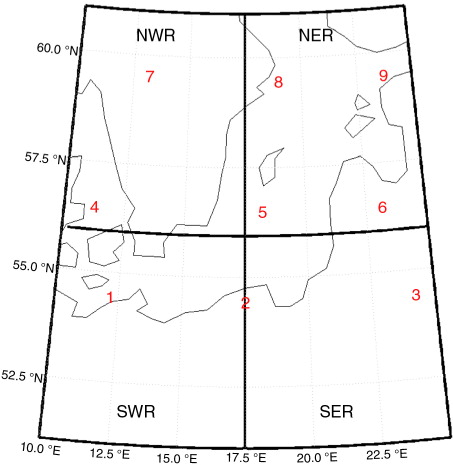
The study is based on a seasonal analysis with seasons defined as: Winter (December, January, February – DJF), Spring (March, April, May – MAM), Summer (June, July, August – JJA) and Autumn (September, October, November – SON). Autumn and winter are typically the seasons with the highest wind speeds over the Baltic Sea (also found in this study).

We use two definitions for mean wind. Definition (1) considers the three events per season which are closest to the 50th percentile of wind speed (hereafter named ‘median wind events’). Note that this definition is not the statistical ‘median’, because we use the three events closest to the 50th percentile of wind speed. This measure is used to ensure comparability with the definition of extreme events, which also includes no more than three events per season. Definition (2) considers the average of available daily data in the time period of interest (hereafter named: ‘average wind events’). This definition is only used for the empirical orthogonal function (EOF) analysis in Section 4.3. We use a different ‘mean’ for the EOF analysis to increase the sample size and ensure robustness of the EOF patterns, which would be smaller with only three events per season. Nevertheless, we also conduct the analysis with the ‘median wind events’ definition and obtained similar patterns, but without any significant trends.

The extreme winds are defined by choosing a percentile threshold. In Section 4.1, we define the three strongest events per season as ‘extreme wind events’. For the monthly analysis of wind direction frequencies in Section 4.2, the threshold to define the extremes was the 90th percentile. Applying a higher percentile would reduce the number of extreme events per month compromising the robustness of this statistic. Hence, every month includes approximately three extreme events. For the EOF analysis in Section 4.3, the 98th percentile is used.

2.4. Statistical methods

One statistical method applied in this study is the principal component (PC) analysis, also known as the empirical orthogonal function (EOF). This analysis derives the dominant patterns of variability (von Storch and Zwiers, 1999). Note that the EOF analysis is applied to anomalies, that is, deviations from the long-term mean.

Rogers’ (1990) analysis of European SLP with the EOF method enables the determination of four main pressure patterns. He used this method to capture most of the variability of the daily pressure fields with just a few patterns.

In Section 4.3, we use this method to identify and compare seasonal wind field patterns for mean and extreme wind events. In case of the mean wind events, we determine monthly anomalies of the zonal (u) and of the meridional (v) wind component based on the available daily data. The gridded fields of the wind components u and v are concatenated into one field, resulting in twice the dimension of the original fields. The EOF analysis is applied to this augmented field.

In case of the extreme events, we calculate the seasonal 98th percentile of wind speed for the field mean of the Baltic Sea region. The u and v components on days above these percentile values are averaged, as the EOF analysis is applied to anomalies. These averages are used to determine the anomalies of u and v by subtracting them from the seasonal extremes, and hence the anomalies are not calculated by subtracting the long-term mean of the entire sample of winds.

The complex correlation coefficient is a method to determine the co-variability between two vector fields (von Storch and Zwiers, 1999). A two-dimensional vector time series can be represented as a complex time series, where the real and imaginary components are given by the first and second dimensions of the vector m=u+iv. Given two two-dimensional vector time series m=(u _m (t), v _m (t)), and e=(u _e (t), v _e (t)), the complex correlation r _c is defined as the complex Pearson correlation between the two complex time series:1 $r_{\text{c}}=\frac{\sum (m_t*e_t^{*})}{\sqrt{\sum (m_t*m_t^{*})\sqrt{\sum (e_t*e_t^{*})}}}$1

where the superscript * denotes the complex conjugate. The result r _c is again a complex number. The complex correlation coefficient can be characterised by its magnitude, which describes the strength of the linear relationship between the magnitude of the vectors, and by a phase angle, which describes the average direction difference between both vector time series. This phase angle is the advantage of the complex correlation compared to a normal correlation, allowing the determination of the directional relationship between two vectors. Kundu (1975) applied this method to investigate the Ekman veering in the Pacific Ocean at the coast of Oregon (USA). In our case, the complex correlation is calculated between the monthly mean winds m and the monthly extreme winds e, and thus provides a measure of the coupling of the variations in magnitude and direction between mean winds and extreme winds.

3. Comparison of coastDat2 and HiResAFF

In the following, the wind characteristics in the two data sets are compared in their overlapping period from 1948 to 2009. Although the overall aim of this study is the comparison of changes in wind direction statistics, the comparison of both data sets will also be focused on statistics of wind speeds. This section provides a general assessment of the comparability of the wind variable of both data sets.

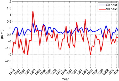
Mean wind events (50th percentile of wind speed, Section 2.3) and extreme wind events (98th percentile of wind speed) per season were determined. As an illustration, Fig. 2 shows the differences between mean wind speeds of coastDat2 and HiResAFF (negative values indicate higher values for HiResAFF) for the 50th and 98th percentiles in winter, displaying larger differences for the 98th percentile. These differences appear in all seasons, which leads to the conclusion that HiResAFF produces higher extreme wind speeds than coastDat2 during all seasons.

Fig. 2 Difference of the 50th percentiles (blue) and 98th percentiles (red) of wind speed between coastDat2 and HiResAFF data sets during winter (DJF). The figure displays the mean over the area shown in Fig. 1.

For winter, summer and autumn, HiResAFF systematically presents higher values with respect to coastDat2 for mean and for extreme winds. In spring, the mean winds in HiResAFF are weaker, but extreme winds are stronger than in coastDat2. All seasons show higher deviations of HiResAFF with respect to coastDat2 in extreme wind events. Figure 3 shows this comparison for the winter season.

Fig. 3 Scatter plot of the 50th (upper) and 98th (lower) percentiles of wind speed of each winter for coastDat2 and HiResAFF for the period 1948–2009. The blue line represents the linear regression and the light grey line the one-to-one-correspondence line. The figure shows the mean over the area displayed in Fig. 1. STD - standard deviation; c - coastDat2; h – HiResAFF.

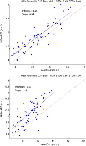
The standard deviations (STD) for the 98th percentile are higher than for the 50th percentile for all seasons and in both data sets. The coefficient of variation (STD/mean) of the two data sets coastDat2 and HiResAFF is almost the same ($\simeq 0.47$).

Subsequently, several tests were conducted to compare the data sets more quantitatively. These comparisons between both data sets are conducted to document the main differences found in our analysis of the wind and illustrate the uncertainty stemming from the use of different gridded products. The comparisons are not meant as a thorough critical analysis of the advantages or deficiencies of one data set over the other, which would require a comparison between the two underlying regional models, CCLM and RCAO that were used to produce these data. This is beyond the scope of the present study. For instance, the distribution of extremes probably deviates from a normal distribution and therefore a more sophisticated test than the F-test would be required. Nevertheless, these tests can provide useful guidelines for further studies.

First, a Student's t-test, which tests the hypothesis that two samples have equal means, is conducted. This hypothesis of equal means could be rejected at the 95% level of significance for most parts of the area, both for the 50th as well as for the 98th percentile. Second, the ratio of variances is tested with an F-test. The hypothesis of equal variances can be rejected in about half of the area for the 50th percentile wind at the p=0.05 level and cannot be rejected in most areas for the 98th percentile. Third, a Kolmogorov–Smirnov test, which tests the hypothesis that two samples are drawn from the same continuous distribution, is applied. This hypothesis of equal distributions is rejected at the p=0.05 level for all seasons. This test is repeated after subtracting the mean, and this reveals that, in this case, the null hypothesis of same continuous distributions cannot be rejected (p≈0.3). This indicates that both data sets preponderantly differ in their means but not in their distribution. However, differences between both data sets are not surprising, as both data sets are based on different dynamical models, each with their own systematic biases.

Both data sets incorporate information from observations and aim at replicating the observed time evolution of winds. Therefore, they can also be compared by the mutual (complex) time correlation (see Section 2.4). The magnitude of the complex correlation coefficient of the area-averaged wind is, for all seasons, significant and higher than 0.7. This demonstrates that the variations in wind magnitude are coherent in both data sets. Furthermore, the phase angle of the complex correlation is always below 0.05°, meaning that the time variations in the wind directions are coherent in both data sets.

4. Comparison of mean and extreme wind statistics

4.1. Differences in directions

The distribution of wind intensity and wind direction is analysed by wind roses for each season in order to investigate differences between wind directions of median and extreme wind events (following the definitions in Section 2.3). The results are summarised in Fig. 4. The analysis here is based on coastDat2 wind data (1948–2009), with the main differences obtained in the analysis of HiResAFF presented later.

Fig. 4 Wind roses of median (left: a, c, e, g) and extreme (right: b, d, f, h) wind in coastDat2 (1948–2009). The colours show the intensity (in m s⁻¹) and the bins show the direction from which the wind blows. Median events are defined as the three wind events per season which are closest to the 50th percentile of wind speed. Extremes are determined as the three strongest wind events per season.

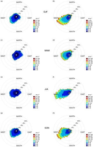
For median wind events, the main wind direction varies across the seasons: In wintertime (Fig. 4a), median winds are clearly dominated by SW wind. Spring (Fig. 4c) shows two main directions, namely E and NE with a secondary maximum for SW directions. In summer (Fig. 4e), the wind tends to blow from W, NW and SW. In autumn (Fig. 4g), the wind mostly blows from SW with a second maximum from SE.

The distribution of extreme wind directions (Fig. 4b, d, f and h) deviates from the distribution of median wind directions. All seasons are dominated by SW winds, and only in spring (Fig. 4d) is there a tendency of more frequent W winds and a weak secondary maximum from north–north–east (NNE). Thus, according to the analysis of seasonal wind roses, median wind directions seem to have a much more isotropic distribution than extreme wind directions. Extreme wind directions are focused mainly on SW and W directions during all seasons.

The analysis is repeated with the HiResAFF data set in the overlapping period (1948–2009). In the case of median winds, the results obtained with HiResAFF also display, as in coastDat2, a much more isotropic distribution of wind directions. The result confirms that the distribution of extreme wind directions is skewed to the south-western directions.

The analysis of the longer period 1850–2009 in HiResAFF shows more isotropic median wind events, with bins forming almost a circle. These wind roses are smoother due to the higher number of events included in the analysis of 160 yr (instead of 65 yr). For extreme wind events, stronger westerly than south-westerly winds are found (not shown).

We analysed the co-variation between median and extreme wind directions by the complex correlation coefficient between both (calculated as described in Section 2.4). The result shows no significant temporal correlation (r≤0.25) for all seasons, which points to a small co-variation between median and extreme wind directions. In conclusion, it does not seem possible to simply infer information of anomalous directions of extreme wind directions from the anomalous directions of median wind.

4.2. Regional differences

So far we have compared the distributions of median and extreme winds as averages over the whole Baltic Sea region. In this section, we explore the possibility that these relationships may be spatially heterogeneous by investigating differences in Baltic Sea subregions. These subregions are hereafter indicated as south-western (SWR), south-eastern (SER), north-western (NWR) and north-eastern (NER) (see Section 2.3 for geographical information). Again, we show first the main results obtained with coastDat2 wind data (1948–2009). To reasonably separate the area into subregions, we compare wind roses (not shown) at nine points scattered across the area (Fig. 1, see also Section 2.3).

Percentile calculations are separately applied to each month of coastDat2 (1948–2009) (see also Section 2.3). As explained below, for median wind events (50th percentile), differences among the subregions can rather be found between North and South than between East and West. For extreme wind events (three strongest days per season, see also Section 2.3), there are no spatial differences in autumn and winter, where all nine points are dominated by SW and W winds. Spring and summer again show mainly differences between North and South. This analysis thus supports the choice of subdividing the investigation area into North and South. However, we decided to subdivide the whole region into four equal subregions so as to capture possible minor differences between East and West (Fig. 1).

For median wind directions, there is a notable absence of a seasonal cycle in all subregions. Figure 5 shows the annual cycle of the eight main wind directions for median wind events for the south-western region as illustration for the behaviour of all other regions.

Fig. 5 Annual cycle of the eight main wind directions of coastDat2 (1948–2009) for the south-western Baltic Sea region (SWR in Fig. 1). This figure only includes the three wind events per month with intensities closest to the 50th percentile of wind speed per month. Units are monthly mean frequency in %.

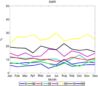
Figure 6 shows the annual cycle of the eight main wind directions (N, NE, E, SE, S, SW, W, NW) for the extreme wind events, averaged over each of the four selected subregions (Fig. 1). In all four subregions, W and SW are the dominant wind directions for extreme wind events in all seasons, with SW winds being more frequent in winter and autumn and less frequent in spring and summer. SE and S wind frequencies have only little variations across all four regions. Beyond this, the regions display some specific characteristics. The southern regions (Fig. 6c and d) show high frequencies of W wind during spring and summer. The northern regions, in contrast, feature a different main direction in spring, with dominant N and NE winds (Fig. 6a and b).

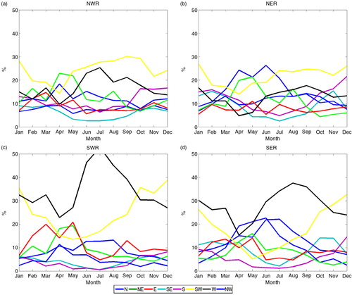
Fig. 6 Annual cycle of the eight main wind directions for extreme events of coastDat2 (1948–2009) in (a) north-western (NWR), (b) north-eastern (NER), (c) south-western (SWR) and (d) south-eastern (SER) Baltic Sea (see Fig. 1). Extremes are defined by the 90th percentile of wind speed per month. Units are monthly mean frequency in %.

The analysis for median and extreme winds is also conducted with the HiResAFF data set in the overlapping time period (1948–2009) to test the robustness of the results based on coastDat2 wind data. Median winds in HiResAFF show directions with almost the same frequency in all subregions (comparable to coastDat2 Fig. 5) and there is very little intra-annual variation. Extreme wind events in the eastern regions (NER, SER) also show a predominance of SW directions, whereas extreme winds in the western regions (NWR, SWR) show slightly lower (5–7%) frequencies for SW winds compared to coastDat2. In these western regions, extreme winds from W show higher frequencies in the order of 10–15%. Nevertheless, for HiResAFF, extreme winds from W show highest frequencies in all regions. Thus, HiResAFF shows a stronger zonal component.

Summarising, the southern regions display higher frequencies of extreme winds for SW and W winds and lower frequencies for N, NE and NW than the northern regions, whereas median winds generally display a more isotropic distribution than extreme winds in all subregions.

4.3. Seasonal patterns

In this section, we analyse the spatial co-variability of the wind directions by means of an EOF analysis. This analysis yields the main spatial patterns of anomalies that tend to evolve coherently in time. To conduct the EOF analysis, the zonal wind (u) and meridional wind (v) components are merged into one field with a doubled number of grid cells. The patterns are based on anomalies of monthly mean wind speeds for the average wind statistics and on anomalies of the 98th percentile for extreme wind statistics (see Section 2.4). The EOF analysis is applied to coastDat2 and HiResAFF in their overlapping period (1948–2009) and on longer time scales back to 1850 to HiResAFF.

For the period 1850–2009 the leading three EOF patterns for both average and extreme wind explain at least ≈82% variance for all seasons. The explained variances per season and data set can be found in Table 1.

Table 1. Explained variance in % of the three leading EOF patterns for each season derived from HiResAFF (1850–2009 and 1948–2009) and coastDat2 (1948–2009). Results for monthly mean wind are shown as plain text and results for wind events exceeding the 98th percentile in bold

HiResAFF (1850–2009)	EOF 1	EOF 2	EOF 3	EOF 1+2+3
DJF	65, 41	25, 31	6, 11	96, 82
MAM	58, 38	28, 32	7, 12	93, 82
JJA	50, 48	30, 29	9, 8	89, 86
SON	54, 46	33, 27	7, 11	95, 84
HiResAFF (1948–2009)
DJF	64, 46	25, 25	6, 11	96, 82
MAM	59, 45	29, 31	6, 8	93, 84
JJA	50, 39	29, 33	10, 11	89, 83
SON	61, 43	27, 28	7, 11	95, 82
coastDat2 (1948–2009)
DJF	63, 39	22, 35	8, 9	93, 83
MAM	56, 43	24, 29	8, 11	88, 83
JJA	56, 47	18, 25	13, 11	87, 83
SON	55, 39	27, 36	9, 14	91, 89

As an example, Fig. 7 displays the two leading EOF patterns together with their PC time series for average and extreme wind events (see Section 2.3 for definitions) for the winter season of HiResAFF (1850–2009). The corresponding explained variances are displayed in Table 1.

4.3.1. EOF patterns.

In the following, the resulting EOF patterns are described for each season and time period for HiResAFF (1850–2009), HiResAFF (1948–2009) and coastDat2 (1948–2009). For sake of clarity, this description is based on one polarity of the patterns, although it should be noted that the opposite polarity (the spatial pattern multiplied by −1) would represent the same EOF.

In winter (DJF), the first EOF derived from HiResAFF explains 65% of the average wind event variation over the period 1850–2009 (Table 1) and is defined by west (W) wind anomalies (Fig. 7a). Although the W wind pattern is similar for extreme events (Fig. 7e) the explained variance of 41% (Table 1) is lower.

Fig. 7 First leading EOF patterns together with their PC time series for average wind [upper four panels: (a–d)] and extreme wind [lower four panels: (e–h)] events of the HiResAFF data set (1850–2009). The left-hand side panels show the pattern of variability of the combined u and v EOF analysis (see Section 2.4). Arrows are not scaled for the sake of clarity. The right-hand side panels show the corresponding principal component time series. The coloured lines in (b) and (h) show trends on different time scales. The significance values (p-values) for the green (g), red (r) and blue (b) lines are shown above the figures. Explained variances are indicated in Table 1.

The result for extreme wind patterns is generally confirmed by the analysis of HiResAFF for the period 1948–2009 (not shown) with a slightly higher explained variance of 46%. Mean wind events indicated a shift to more south-westerly winds in the period 1948–2009. This result is confirmed in the analysis of coastDat2 (1948–2009; not shown). This data set results in a similar direction of wind anomalies as HiResAFF in 1948–2009, both for average and extreme wind patterns. The use of coastDat2 exhibits a predominance of SW anomalies and slightly lower explained variances of 63% for average winds and 39% for extreme winds when compared to HiResAFF.

For spring (MAM; not shown), the EOF patterns of average winds in all data sets show predominantly SW anomalies, with an explained variance of approximately 56%. For extreme winds, the results differ between each data set: whereas the HiResAFF pattern exhibits a preponderance of westerly wind anomalies (W) for the period 1850–2009 and south-easterly anomalies (SE) for the period 1948–2009, the pattern resulting from the coastDat2 data results, as in the case of winter season, in south-west (SW) anomalies.

The summer season (JJA; not shown), for average and extreme winds, displays a SW pattern of wind anomalies for all data sets and all periods. Autumn (SON; not shown) reveals a similar pattern of anomalies of main wind directions as for winter: the HiResAFF pattern obtained in 1850–2009 mainly indicates W wind anomalies for averages and for extremes. For the time period 1948–2009, average and extreme wind anomaly patterns are characterised for both data sets (HiResAFF and coastDat2) by SW wind anomalies. Thus, autumn and winter display very similar patterns of wind direction variability, for both the average and extreme events. Note that this does not necessarily mean that the temporal evolution of their variability is correlated.

The second EOF of HiResAFF (1850–2009) displays a pattern of southerly wind anomalies for both average and extreme wind patterns, in all seasons (illustrated here for winter: Fig. 7c and g), with a slightly easterly component in summer. The dominant southerly direction of wind anomalies, for average and extreme winds, is also prominent in HiResAFF for the shorter period 1948–2009 (not shown). However, some seasons slightly deviate from this general rule: JJA average wind and SON extremes have an additional easterly component and extremes for MAM an additional westerly component. CoastDat2 (not shown) average wind anomaly patterns show southerly winds and westerly extreme winds with a northern component for MAM and JJA and a southerly component for SON. For all data sets and periods, the explained variances of the second EOF for extreme events are higher than for average events (Table 1). The difference between the variance explained by the first and second EOF explained variances is much smaller for extremes than for the average winds. Hence the second pattern is, in relative terms, more important for extreme events than for average events.

The third EOF (not shown) is dominated by a cyclonic rotation over the Baltic area with a centre close to the Island of Gotland. The amount of explained variance lies between ≈6% (MAM) and ≈12% (JJA) for average and extreme events in all seasons. Because these values are quite low and the EOF patterns are physically not clear, it can be assumed that these patterns are dominated by noise.

4.3.2. PC time series.

Another result of the EOF analysis is the PC time series, which describes the variations of the amplitude of the spatial patterns through time. The PCs give information about long-term trends in the spatial patterns just described, and also about possible correlations in time of these patterns.

For average winds, the HiResAFF data set (1850–2009) shows significant trends in winter, summer (not shown) and autumn (not shown) for the first PC. There is a significant negative trend in winter (negative for the polarity shown in Fig. 7b) and also a negative trend in summer from 1850 to 1973, followed by a non-significant increase until 1990. These trends are also visible in the period 1948–2009 (not shown) in HiResAFF and coastDat2, however, they are not statistically significant. In autumn, there is a significant increase from 1990 to 2009 for HiResAFF (1850–2009) and HiResAFF (1948–2009), coastDat2 shows a similar trend but without statistical significance.

It is important to note that no significant trends for extreme winds could be detected for the leading PC time series in any season or data set. For the second PC, there is a significant positive trend in winter season from 1940 to 1990, which is only visible in HiResAFF (1850–2009) (Fig. 7h).

We additionally calculate the seasonal correlation between the PC time series of average winds and the PC time series of extreme winds. This correlation shows low values for all seasons between r= − 0.23 and r=0.18 for both data sets (coastDat2, HiResAFF) and both periods (1948–2009, 1850–2009). This suggests that changes of average winds cannot be used to estimate changes of extreme winds. This is also shown in Section 4.1 with the help of the complex correlation between average and extreme winds.

The NAO is one of the leading patterns of seasonal climate variability in this region, especially in winter. It is thus expected that the link between the NAO and the variability of average wind speed is strong, but its link to the variability of extreme wind speeds has not been thoroughly investigated. The seasonal correlation between the leading PC and the NAO index shows comparable results for both time periods and data sets. Therefore, the following correlation coefficients are only shown for HiResAFF (1850–2009): average wind events exhibit an expected high correlation for DJF of 0.64. However, for the other seasons the correlations have much lower values (MAM, 0.28; JJA, 0.17; SON, 0.22), indicating that in seasons other than winter the NAO is not the main factor that modulates the average wind speed. For extreme wind events, the correlations are low for all seasons (DJF, −0.13; MAM, −0.07; JJA, 0.01; SON, 0.04). This somewhat unexpected result indicates that the link between the variability of average wind speed and the variability of extreme winds is not strong.

The comparison of PCs and their corresponding EOF patterns leads to the following conclusions:

The first EOF of average wind describes the most important direction of wind variability. The analysis of the longer period 1850–2009 indicates that the main direction of variability of average winds is the zonal direction (W–E), whereas the analysis of the period from 1948 to 2009 (HiResAFF and coastDat2) reveals that the main direction of variability has turned in the recent decades with an additional meridional component (SW–NE).

The EOFs of extreme winds are derived from the anomalies relative to the average extremes, the patterns describing variations relative to the average of the high percentile winds. Thus, it describes variations in time within the population of extreme winds. The analysis of the period from 1850 to 2009 indicates that the main direction of extreme wind variability is from W–E; however, for the period from 1948 to 2009, the direction has turned to SW–NE. Therefore, concerning the long-term variation of wind directions, average and extreme winds have changed in a similar way over the last decades relative to their long-term mean.

This raises the issue of whether an anomalous direction of winds in a particular season contains information about the expected direction anomalies in the following seasons. The correlation between the seasonal PCs of average winds in adjacent seasons is found to be small. The correlation between the leading autumn PC with the leading winter PC in the same year shows only small values (r≤0.3) for all data sets and periods, suggesting that the intensity of the main pattern of wind direction variability does not tend to persist from one season to the next. This also happens for extreme wind events. Thus, it does not seem possible to statistically predict (with linear methods) seasonal wind conditions from wind information from a previous season in the same year.

The comparison between EOFs derived from HiResAFF and coastDat2 explains a similar amount of variances, but the EOF patterns derived from HiResAFF tend to display a more zonal direction than in the other data sets (also seen for the wind rose analysis in Section 4.1).

5. Discussion and conclusions

Our study focused on the question of whether the variability of mean (median and average) and the variability of extreme wind statistics over the Baltic Sea region are comparable. An assumption could be made that changes in mean wind statistics could be used to approximate extreme wind changes. This study refuses this hypothesis, at least regarding wind direction over the Baltic region.

Our study analysed two regional data sets in the time periods 1850–2009 (HiResAFF) and 1948–2009 (coastDat2) as well as their overlapping time period 1948–2009. Two data sets were utilised in this analysis (HiResAFF and coastDat2). As these two data sets had not previously undergone systematic analysis, the first task necessary was to compare the wind statistics in the common time period. Data collection of each data set differed and different models were used to produce the data sets. However, for the common period of time both were consistent concerning wind directions.

The second part of this study compared mean (median and average) and extreme wind statistics, with a focus on wind direction. Our main conclusions are as follows:

1. Median winds show a very isotropic distribution for all directions with a different maximum in each season. Extreme winds are much more constrained to SW directions for all seasons except spring where a second maximum can be found in NE direction.

2. We found a very weak co-variation of the anomalies of median and of extreme wind over the Baltic Sea region. Anomalous direction of median winds in one particular season and year are thus not indicative of extreme winds displaying the same anomalous direction.

3. A subdivision into four parts of the Baltic Sea region shows regional differences in the behaviour of median and extreme events. Median wind events have quite similar frequencies of direction in all four regions. These frequencies also stay relatively stable across all seasons. Extreme wind events show differences between northern and southern regions. The stormy seasons (DJF, SON) tend to be dominated in all four regions by SW winds. In spring and summer, the northern regions are dominated by north-easterly winds and the southern regions by westerly winds.

4. We address the question of whether there is a persistent annual pattern of wind direction anomalies that persists through adjacent seasons. The temporal evolution of the patterns of seasonal variability, derived from an EOF analysis of the seasonal anomalies, does not show significant correlations between adjacent seasons. Thus it is not possible, within a linear framework, to infer information about the anomalous winds in one season from the anomalous winds in the previous seasons.

Additionally, the long-term evolution of the leading PCs also displays a different behaviour for average and extreme winds. For the first PC (mainly zonal direction), we only found significant long-term changes over time for average wind events, but not for extreme winds, suggesting that whereas the zonal pattern of variability of average winds showed a trend, it showed no changes for extreme winds. Conversely, the second leading PC representing variability in the meridional direction did not change for average winds, but indicated a trend for extremes. The second pattern is more important in terms of explained variance for extreme events than for average events. An increasing trend for the first PCs of average wind is visible for shorter time scales (1948–2009) for both data sets. When analysing the longer time series (1850–2009) it becomes clear that this trend is not present over the whole period. The same effect was found, in numerous studies, for trends of wind speed. Over Europe, many studies found an increase in storm intensity, and therefore also higher wind speeds, between the 1960s and the mid-1990s (Gulev and Hasse, 1999; Gulev et al., 2001; McCabe et al., 2001; Paciorek et al., 2002; Wang et al., 2006). Whereas Bärring and Fortuniak (2009), on longer time scales, show that there is rather interdecadal variability than clearly defined long-term increasing or decreasing trends.

Moreover, we found that the connection between the NAO and the average winds differs from extreme events. The seasonal correlation between the first PC of extreme wind events and the NAO index is very weak. This is in contrast to the correlation between the NAO and the average winds in wintertime. It is known that the NAO has a large influence on the wind conditions over the Baltic Sea, especially during winter (Feser et al., 2014; Rutgersson et al., 2014), so this correlation is not surprising. However, in the other seasons there seem to be other atmospheric driving mechanisms for the variability of average wind speed. Extreme wind events do not show high correlations to the NAO in any season. We conclude that the NAO is not the main driver for extreme winds.

Our results provide insight on the issue of whether, and how, changes in mean wind statistics can be related to changes in extreme wind statistics (Seneviratne et al., 2012). The matter of the existence of long-term trends in extreme winds is also addressed (Donat et al., 2011; Krueger et al., 2013). In a review by Feser et al. (2014), it is stated that trends in storm activity crucially depend on the time scales considered. As storms produce extreme winds, this issue is also related to the present study. Our results concerning wind direction support the statement that trends are dependent on the time span. The extreme events over the longer period in HiResAFF showed the highest frequencies for W winds, whereas for the shorter period covered by both HiResAFF and coastDat2 the distribution of wind direction showed a maximum of SW wind. This result is in agreement with previous studies based on different data sets and without regional subdivisions; for example, Jaagus and Kull (2011) also found a shift towards SW in the wind directions, albeit on shorter time periods (1966–2008). Therefore, when analysing differences in wind statistics between data sets, it is important to ensure that the time periods are the same. Moreover, it is important to keep in mind the different data set uncertainties. Probably, the biggest difference between HiResAFF and coastDat2 is the spectral nudging which is only applied for coastDat2. This method is known to improve reconstructions and lower the difference relative to observations. We argue that the AM contains a higher level of uncertainties. The uncertainties include model uncertainties; noise in the used observations (e.g. measurement errors), also present in reanalysis data sets; dependencies on the analogue pool size; and the link between real and simulated predictors (Schenk and Zorita, 2012).

Furthermore, there are uncertainties due to the different models used to conduct the two reconstructions. Neither the regional model CCLM nor the RCAO model is perfect, but the aim of this study was not to identify the better data set. However, although both data sets have different uncertainties due to different models and methods, both show comparable results regarding the variability of wind direction statistics of mean (median and average) and extreme wind events.

Comparing coastDat2 and HiResAFF, the reader should also keep in mind the impact of, for example, the bias on the EOF analysis. A difference in the mean would change the distribution and hence the variability, as lower mean values in wind speed would induce a more skewed distribution. Although both data sets already showed comparable results, a bias correction could lead to even more similar results, because the different means were identified as the main differences in both data sets.

As mentioned above, both data sets, HiResAFF and coastDat2, showed similar results. However, in the overlapping period (1948–2009) there are differences between both data sets regarding the frequencies of the SW and W wind directions for extreme winds. HiResAFF exhibited higher frequencies for W winds in all Baltic Sea regions. We suggest that this stronger zonal component may be an artefact of HiResAFF, due to the uncertainties mentioned above, but this question requires further study.

The overall conclusion of our study is that the hypothesis that the statistics of mean wind can serve as a proxy for statistics of extreme wind is rejected for the Baltic Sea region.

6. Acknowledgements

The authors thank Dr. Dennis Bray for copy-editing this manuscript. This work is a contribution to the Helmholtz Climate Initiative REKLIM (Regional Climate Change), a joint research project of the Helmholtz Association of German research centres (HGF).

References

- Alexandersson H. , Tuomenvirta H. , Schmith T. , Iden K . Trends of storms in NW Europe derived from an updated pressure data set. Clim. Res. 2000; 14: 71–73.
- Bärring L. , Fortuniak K . Multi-indices analysis of southern Scandinavian storminess 1780–2005 and links to interdecadal variations in the NW Europe–North Sea region. Int. J. Climatol. 2009; 29: 373–384.
- Clemmensen L. B. , Hansen K. W. T. , Kroon A . Storminess variation at Skagen, Northern Denmark since AD 1860: relations to climate change and implications for coastal dunes. Aeolian Res. 2014; 15: 101–112.
- Compo G. P. , Whitaker J. S. , Sardeshmukh P. D. , Matsui N. , Allan R. J. , co-authors . The twentieth century reanalysis project. Q. J. Roy. Meteorol. Soc. 2011; 137(654): 1–28.
- Doescher R. , Willen U. , Jones C. , Rutgersson A. , Meier H. E. M. , co-authors . The development of the regional coupled ocean–atmosphere model RCAO. Boreal Environ. Res. 2002; 7: 183–192.
- Donat M. G. , Renggli D. , Wild S. , Alexander L. V. , Leckebusch G. C. , co-authors . Reanalysis suggests long-term upward trends in European storminess since 1871. Geophys. Res. Lett. 2011; 38: L14703–L14703.
- Feser F. , Barcikowska M. , Krueger O. , Schenk F. , Weisse R. , Xia L . Storminess over the North Atlantic and northwestern Europe – A review. Q.J.R. Meteorol. Soc. 2015; 141: 350–382.
- Geyer B . High resolution atmospheric reconstruction for Europe 1948–2012: coastdat2. Earth Syst. Sci. Data. 2014; 6: 147–164.
- Gulev S. K. , Hasse L . Changes of wind waves in the North Atlantic over the last 30 years. Int. J. Climatol. 1999; 19: 1091–1117.
- Gulev S. K. , Zolina O. , Grigoriev S . Extratropical cyclone variability in the Northern Hemisphere winter from the NCEP/NCAR reanalysis data. Clim. Dynam. 2001; 17: 795–809.
- Hurrell J . Decadal trends in the North Atlantic Oscillation – regional temperatures and precipitation. Science. 1995; 269: 676–679.
- Jaagus J . Kont A. , Tõnisson H . Long-term changes in frequencies of wind directions on the western coast of Estonia. 2009. Climate Change Impact on Estonian Coasts, Tallinn University, Tallinn, Estonia (in Estonian, with Englisch summary).
- Jaagus J. , Kull A . Changes in surface wind directions in Estonia during 1966–2008 and their relationships with large-scale atmospheric circulation. Estonian J. Earth Sci. 2011; 60: 220–231.
- Jacob D. , Podzun R . Sensitivity studies with the regional climate model REMO. Meteorol. Atmos. Phys. 1997; 63: 119–129.
- Kalnay E. , Kanamitsu M. , Kistler R. , Collins W. , Deaven D. , co-authors . The NCEP/NCAR 40-year reanalysis project. Bull. Am. Meteorol. Soc. 1996; 77: 437–471.
- Keevallik S . Wind speed and velocity at three Estonian coastal stations 1969–1992. Estonian J. Eng. 2008; 14: 209–219.
- Keevallik S . Shifts in meteorological regime of the late winter and early spring in Estonia during recent decades. Theor. Appl. Climatol. 2011; 105: 209–215.
- Kent E. C. , Fangohr S. , Berry D. I . A comparative assessment of monthly mean wind speed products over the global ocean. Int. J. Climatol. 2013; 33: 2520–2541.
- Kistler R. , Kalnay E. , Collins W. , Saha S. , White G. , co-authors . The NCEP/NCAR 50-year reanalysis: monthly means CD–ROM and documentation. Bull. Am. Meteorol. Soc. 2001; 82: 247–267.
- Krueger O. , Schenk F. , Feser F. , Weisse R . Inconsistencies between long-term trends in storminess derived from the 20CR reanalysis and observations. J. Clim. 2013; 26: 868–874.
- Krueger O. , von Storch H . Evaluation of an air pressure-based proxy for storm activity. J. Clim. 2011; 24: 2612–2619.
- Kruizinga S. , Murphy A. H . Use of an analogue procedure to formulate objective probabilistic temperature forecasts in The Netherlands. Mon. Weather Rev. 1983; 111: 2244–2254.
- Kull A . Relationship between inter-annual variation of wind direction and wind speed. Publicationes Instituti Geographici Universitatis Tartuensis. 2005; 97: 62–70.
- Kundu P. K . Ekman veering observed near the ocean bottom. J. Phys. Oceanogr. 1975; 6: 238–242.
- Lehmann A. , Getzlaff K. , Harla J . Detailed assessment of climate variability of the Baltic Sea area for the period 1958–2009. Clim. Res. 2011; 46: 185–196.
- Lorenz E. N . Atmospheric predictability as revealed by naturally occurring analogs. J. Atmos. Sci. 1969; 26: 639–646.
- McCabe G. , Clark M. , Serreze M . Trends in Northern Hemisphere surface cyclone frequency and intensity. J. Clim. 2001; 14: 2763–2768.
- McVicar T. , Roderick M. , Donohuea R. , Lia L. , Van Nielc T. , co-authors . Global review and synthesis of trends in observed terrestrial near-surface wind speeds: implications for evaporation. J. Hydrol. 2012; 416–417: 182–205.
- Nilsson C . Windstorms in Sweden – Variations and Impacts. 2008. PhD Thesis. Lund University, Lund, Sweden.
- Paciorek C. , Risbey J. , Ventura V. , Rosen R . Multiple indices of Northern Hemisphere cyclone activity, winters 1949–99. J. Clim. 2002; 15: 1573–1590.
- Raible C. , Yoshimori M. , Stocker T. F. , Casty C . Extreme midlatitude cyclonesand their implications for precipitation and wind speed extremes in simulations of the maunder minimum versus present day conditions. Clim. Dynam. 2007; 28: 409–423.
- Reckermann M. , Langner J. , Omstedt A. , von Storch H. , Keevallik S. , co-authors . Baltex – an interdisciplinary research network for the Baltic Sea region focus on environmental, socio-economic and climatic changes in Northern Eurasia and their feedbacks to the global earth system. Environ. Res. Lett. 2011; 6: 045205.
- Reimann T. , Tsukamoto S. , Harff J. , Osadczuk K. , Frechen M . Reconstruction of Holocene coastal foredune progradation using luminescence dating – an example from the Swina barrier (southern Baltic Sea, NW Poland). Geomorphology. 2011; 132: 1–16.
- Rockel B. W. , Hense A . The regional climate model COSMO-CLM (CCLM). Meteorol. Z. 2008; 12: 347–348.
- Rogers J. C . Patterns of low-frequency monthly sea level pressure variability (1899–1986) and associated wave cyclone frequencies. J. Clim. 1990; 3: 1364–1379.
- Rutgersson A. , Jaagus J. , Schenk F. , Stendel M . Observed changes and variability of atmospheric parameters in the Baltic Sea region during the last 200 years. Clim. Res. 2014; 61: 177–190.
- Rutgersson A. , Jaagus J. , Schenk F. , Stendel M. , Bärring L. , co-authors . Second Assessment of Climate Change for the Baltic Sea Basin, chapter Recent Change – Atmosphere. 2015; 69–97. Springer International Cham Heidelberg, New York Dordrecht London.
- Schenk F. , Zorita E . Reconstruction of high resolution atmospheric fields for Northern Europe using analog-upscaling. Clim. Past. 2012; 8: 1–23.
- Seneviratne S. , Nicholls N. , Easterling D. , Goodess C. , Kanae S. , co-authors . Field C. B. , Barros V. , Stocker T. F. , Qin D. , Dokken D. J. , co-editors . Changes in climate extremes and their impacts on the natural physical environment. Managing the Risks of Extreme Events and Disasters to Advance Climate Change Adaptation. 2012. Special Report of Working Groups I and II of the Intergovernmental Panel on Climate Change (IPCC). Technical Report, Cambridge University Press, Cambridge, UK.
- Siegismund F. , Schrum C . Decadal changes in the wind forcing over the North Sea. Clim. Res. 2001; 18: 39–45.
- van den Dool H . Searching for analogs, how long must we wait?. Tellus A. 1994; 46: 314–324.
- von Storch H. , Langenberg H. , Feser F . A spectral nudging technique for dynamical downscaling purposes. Mon. Weather Rev. 2000; 128: 3664–3673.
- von Storch H. , Zwiers F. W . Statistical Analysis in Climate Research. 1999; Cambridge, UK: Cambridge University Press.
- Wang X. , Swail V. , Zwiers F . Climatology and changes of extratropical cyclone activity: comparison of ERA-40 with NCEP–NCAR reanalysis for 1958–2001. J. Clim. 2006; 19: 3145–3166.
- Weisse R. , Bisling P. , Gaslikova L. , Geyer B. , Groll N. , co-authors . Climate services for marine applications in Europe. Earth Perspect. 2015; 2(3): 1–14.
- Weisse R. , Gaslikova L. , Geyer B. , Groll N. , Meyer E . Coastdat – model data for science and industry. Die Küste. 2014; 81: 5–18.
- Weisse R. , von Storch H . Marine Climate and Climate Change. Storms, Wind Waves and Storm Surges. 2009; Springer Verlag Berlin Heidelberg, New York.
- Weisse R. , von Storch H. , Callies U. , Chrastansky A. , Feser F. , co-authors . Regional meteorological-marine reanalyses and climate change projections: results for northern Europe and potentials for coastal and offshore applications. Bull. Am. Meteorol. Soc. 2009; 90: 849–860.