Application of 3-D ensemble variational data assimilation to a Baltic Sea reanalysis 1989–2013

Abstract

A 3-D ensemble variational (3DEnVar) data assimilation method has been implemented and tested for oceanographic data assimilation of sea surface temperature (SST), sea surface salinity (SSS), sea ice concentration (SIC), and salinity and temperature profiles. To damp spurious long-range correlations in the ensemble statistics, horizontal and vertical localisation was implemented using empirical orthogonal functions. The results show that the 3DEnVar method is indeed possible to use in oceanographic data assimilation. So far, only a seasonally dependent ensemble has been used, based on historical model simulations. Near-surface experiments showed that the ensemble statistics gave inhomogeneous and anisotropic horizontal structure functions, and assimilation of real SST and SIC fields gave smooth, realistic increment fields. The implementation was multivariate, and results showed that the cross-correlations between variables work in an intuitive way, for example, decreasing SST where SIC was increased and vice versa. The profile data assimilation also gave good results. The results from a 25-year reanalysis showed that the vertical salinity and temperature structure were significantly improved, compared to both dependent and independent data.

• data assimilation
• physical oceanography
• Baltic Sea
• reanalysis

1. Introduction

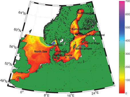
The Baltic Sea is a large estuary with positive water balance, which means that precipitation exceeds evaporation. High-saline water from the North Sea can only be imported through the narrow and shallow Danish straits (see the map in Fig. 1). This implies that the dense deepwater in the Baltic proper interior is only exchanged intermittently, leading to stagnation periods in the Baltic proper with lengths up to about 10 yr. Due to intermittent inflows of high-saline water as well as annual variability of river runoff, the salinity of the Baltic Sea varies on many time scales. Furthermore, due to the stratification in the Baltic Sea, the spatial scales are usually much smaller than in the open ocean, as the internal Rossby radius is about 2–11 km (Alenius et al., 2003; Osinski et al., 2010).

Fig. 1 Model domain, showing depth in metres, names of subregions and the location of the hydrographic stations BY5 and BY15.

The near-surface temperature in the Baltic is highly dependent on the atmospheric forcing and its natural variability on many time scales. Furthermore, the temperature in the deepwater and at intermediate depths also depends on the temperature of the intermittent, inflowing water through the Danish Straits, also leading to variability on many time scales. The atmospheric forcing also leads to upwelling situations near coasts, wind and wave-induced near-surface mixing as well as convection at night-time and during autumn and winter, tending to redistribute the heat and salt of the Baltic. For a more thorough description of the oceanography of the Baltic Sea, see, for example, Leppäranta and Myrberg (2009).

From a climatological point of view, it is both important and interesting to analyse the decadal changes of, for example, temperature and salinity (T/S) distributions in any water body, including the Baltic Sea. National measuring programmes over many decades have accumulated an important data set of T/S profiles, sea surface temperature (SST) and sea surface salinity (SSS) from many locations in the Baltic Sea, as well as other variables such as sea surface height (SSH) along coasts and sea ice concentration (SIC) in terms of ice charts and satellite measurements. As a complement, model simulations have been made covering the last decades, usually forced by down-scaled atmospheric model runs of varying quality.

The advantage of observations is that they represent the true state of the ocean, within measurement errors, but there is always an uncertainty regarding how representative each measurement is for the local area. To make statements about the Baltic Sea as a whole (e.g. mean temperature), it is necessary to interpolate over long distances, between measurement locations and also interpolate in time. It is not uncommon that a measurement station is visited only once a month and is located more than 100 km from neighbouring measurement stations. Some areas may even lack observations for very long time periods. On the other hand, model simulations are usually good at exactly the things that observations are bad at, namely the resolution in time and space, whereas in a model simulation there is no guarantee that the model does not deviate rather far from reality, due to errors and limitations in the model and the atmospheric forcing. Therefore, it is preferable to combine the two, to make a synthesis of model data and observation data, and to get the best out of the two worlds: a homogeneous data set with high resolution in time and space simultaneously following a model trajectory reasonably close to observations. This can be achieved with a process called data assimilation, in which observations are used to update the circulation model to keep it from deviating too far away from reality.

Data assimilation is applied at many operational oceanographic centres in the world, to create high-quality ocean forecasts. This has resulted in valuable data sets covering the last 10–15 yr or so. However, there are some disadvantages of operational data sets. First, over a 10- to 15-yr period, the resolution of the circulation model is likely to have changed (improved) at least once, due to continuous efforts to always giving the best possible product. Second, the quality (resolution, etc.) of the atmospheric forcing has probably improved as well during the same period, for similar reasons. Third, it is also possible that the data assimilation system being applied has changed too, as well as other factors like the number of forecasts per day which may have been increased. All these factors imply that although the operational data sets are of high value, having high resolution and staying relatively close to reality, they are not perfectly homogeneous in the sense that the system has changed, typically many times, over the time period. Furthermore, some observations cannot be used in operational forecasts, simply because they are not yet available at the start of the forecast. Finally, the typical time period of an operational forecast data set (using data assimilation), being 10–15 yr, is not long enough to be used for climate studies.

For these reasons, it has become common to make so-called reanalyses of longer time periods, often stretching back to the time before operational forecasts using data assimilation were available. In meteorology this has been done many times for the global atmosphere, for example, the 40-yr NCEP/NCAR data set (Kalnay et al., 1996); the ECMWF data sets – ERA-15 (Gibson et al., 1997), ERA-40 (Uppala et al., 2005) and ERA-interim (Dee et al., 2011); the Japanese data sets – JRA-25 (Onogi et al., 2007) and JRA-55 (Ebita et al., 2011); and the international effort leading to the 140-yr data set – 20CR (Compo et al., 2011). Higher resolution atmospheric reanalyses for the Baltic region have also been made. The BaltAn65+ reanalysis (Luhamaa et al., 2011) has 11 km grid resolution and covers the Baltic Sea, but only the eastern part of the North Sea. The recent project Euro4M has resulted in a data set of 22 km grid resolution and covers a larger domain for the time period 1979–2013 (Dahlgren et al., 2014).

Oceanographic reanalysis work typically started much later. The first one for the Baltic Sea was BSRA-15, made by one of the present authors in 2005 (Axell, 2013) using the successive corrections data assimilation method (e.g. Daley, 1991), covering the period 1990–2004. It was then followed by two 20-yr reanalyses made during the MyOcean-1 project, both covering 1990–2009. The first one of these, by Fu et al. (2012), used 3-D variational (3DVar) data assimilation, and the second one, by one of the present authors, used univariate optimal interpolation (OI) as data assimilation method (e.g. Daley, 1991). Recently, a 30-yr reanalysis covering 1970–1999 was made by Liu et al. (2013), using multivariate ensemble optimal interpolation (EnOI) in the data assimilation (Oke et al., 2002; Evensen, 2003). Hence, there is a tendency not only for the lengths of the Baltic reanalyses to increase but also for the use of more advanced data assimilation methods.

Apart from the EnOI method mentioned above, other ensemble methods include, for example, the ensemble Kalman filter (EnKF) introduced by Evensen (1994, 2003), the singular evolutive extended Kalman (SEEK) filter (Pham et al., 1998), the ensemble transform Kalman filter (ETKF) introduced by Wang and Bishop (2003) and the singular evolutive interpolated Kalman (SEIK) filter (Nerger et al., 2005). In traditional 3DVar (Parrish and Derber, 1992; Courtier et al., 1998), however, the background error covariances (BECs) are often homogeneous and isotropic as well as static (Gustafsson et al., 2001; Buehner et al., 2010a; Liu and Xiao, 2013), even though in reality they should be flow dependent (Hamill et al., 2002). However, several 3DVar implementations have been made with more realistic BECs. Examples include not only the approaches by Fisher and Courtier (1995) and Buehner et al. (2010a), Buehner et al. (2010b) but also the approaches using so-called hybrid schemes, for example, a mixture between EnKF and 3DVar (Hamill and Snyder, 2000), a mixture between ETKF and 3DVar (Wang et al., 2008), or schemes in which the BEC term in the cost function in 3DVar is replaced by a linear combination of the original BEC term and a new BEC term based on ensemble covariances (Buehner, 2005; Gustafsson et al., 2014).

The merits of using EnKF (which has flow-dependent BECs) and traditional 4-D variational (4DVar) (which has stationary but full rank BECs and allows for direct assimilation of, for example, satellite irradiances) have been discussed by several authors (e.g. Lorenc, 2003; Gustafsson, 2007) and will not be repeated here. Suffice it to say that a combination of both methods would be preferable (Gustafsson and Bojarova, 2014).

A rather new data assimilation method, 4-D ensemble variational (4DEnVar) data assimilation, was recently developed and tested by Liu et al. (2008, 2009) in simplified atmospheric experiments. Large-scale atmospheric experiments using real observations were done later by, e.g. Buehner et al. (2010b), Liu and Xiao (2013), Gustafsson and Bojarova (2014) and Wang and Lei (2014). These authors compared the results with other methods (EnKF, 3DVar, 3DVar-FGAT, Ensemble-based 3DVar, 4DVar, Hybrid 4DVar). The general result was that 4DEnVar was comparable or sometimes superior to the other methods. However, the important points are that (1) in 4DEnVar, no tangent linear or adjoint versions of the model code have to be used, which are both difficult and laborious to obtain and maintain, and that, as a result, (2) the computational cost compared to 4DVar is decreased (Gustafsson and Bojarova, 2014).

The intention of the present paper is to describe an implementation of 3DEnVar in a full operational oceanographic forecasting system and test it by applying it on a 25-yr Baltic Sea reanalysis experiment. To the best of our knowledge, 3DEnVar (or 4DEnVar) has never been applied in oceanography before. Furthermore, the oceanographic case is different than the atmospheric case because of the presence of sea ice, which is a very difficult variable to assimilate. The reason is that sea ice variables are very nonlinear, the associated length scales are very short compared to, for example, temperature, and that the frequency distribution is bimodal rather than Gaussian as it is constrained by nature to be in the range 0–1. The ensemble we will use in this paper is stationary and will be based on model states from previous years but from the same season as the analysis. In this way, the BECs will vary slowly with the seasons. The long-term goal, however, is to implement 4DEnVar and use BECs based on an updated ensemble forecast, but this has not been done in this paper. The method has several interesting properties which may be important in operational forecasts as well as in reanalyses. First, it is by default a multivariate method, which means that one single observation may affect many different variables simultaneously. This may be important in, for example, assimilation of sea ice, in cases where many ice variables cannot be observed. This was also the case in the EnOI method employed by Liu et al. (2013) mentioned above. Second, just like in EnOI, an ensemble of model states is used to calculate statistics for the BECs, which is important to be able to spread the influence of each observation to other points in space as well as to other variables. In addition, being a variational method (like traditional 3DVar and 4DVar, but unlike, for example, EnOI and EnKF), the updated initial field (the analysis) is obtained by minimizing a cost function. This implies that it is possible to assimilate also quantities that are not model variables, for example, integrated quantities such as the transport through a section or radial velocities. This is not easily done with, for example, the OI or EnOI methods.

This paper is organized as follows. First, a description of the circulation model is given in Section 2, followed by a summary of the data assimilation method in Section 3, including the minimization technique, localization and choice of ensemble. In Section 4, we present results from some assimilation experiments including a 25-yr reanalysis experiment. Then the paper concludes with a summary and a discussion of the results in Section 5.

2. The circulation model: HIROMB

The implementation of 3DEnVar described in this paper has so far been adapted for use with two different ocean models. One of them is Nucleus for European Modelling of the Ocean (NEMO), described by Madec and the NEMO team (2008), and the other one is High-Resolution Operational Model for the Baltic (HIROMB). In this paper, we have used HIROMB as the circulation model.

HIROMB is the operational ocean forecasting model in use today at our institute, the Swedish Meteorological and Hydrological Institute (SMHI), and has been since the mid-1990s. Version 2.0 of the model was described by Wilhelmsson (2002) and Funkquist and Kleine (2007), and the changes leading to version 3.0 was described by Axell (2013). In this study, we have used the latest version of HIROMB, v4.6, which compared to v3.0 has improved air–sea interaction, ice dynamics and thermodynamics, and has a rotated grid implemented.

The region covered by the HIROMB configuration used in this study is the North Sea and the Baltic Sea with 5.5 km horizontal grid resolution (see Fig. 1). It has 50 vertical layers (z coordinates) with a cell thickness of 4 m in the upper 80 m of the water column, then slowly increasing to a maximum of 40 m below 360 m depth. The boundary conditions necessary are SSH, salinity and temperature (S/T) profiles, and ice variables. At the open boundaries, a sponge layer is used for all tracers (salinity, temperature, ice) between the inner model grid and the prescribed values at the boundary. For velocities, a radiation condition is applied at the boundary. The open boundary is located in the western English Channel and the northern North Sea (see Fig. 1). SSH is extracted from a storm-surge model called NOAMOD run at SMHI, covering the north-eastern part of the North Atlantic with 44 km grid resolution. The S/T profiles are just climatology in these experiments, and the ice variables are all assumed to be zero (no ice).

The meteorological forcing used in the experiments described here was High-Resolution Limited Area Model (HIRLAM) with 22 km grid resolution, from the recent reanalysis project Euro4M (Dahlgren et al., 2014). The meteorological variables used as forcing are air pressure, wind components, air temperature, humidity and total cloudiness. In HIROMB, precipitation is assumed to be balanced by evaporation. This implies an underestimate of the freshwater forcing of about 10 % (e.g. Omstedt and Axell, 1998) which needs to be corrected by data assimilation in longer simulations.

River runoff to the model is specified using hindcast data from the hydrological forecast model E-HYPE (Arheimer et al., 2012), run operationally at SMHI. The number of rivers is of the order of a few hundred along the model coast line.

The turbulence model is a state-of-the-art two-equation model of the type k - ω (Wilcox, 1998), which has been adapted for ocean applications by Umlauf et al. (2003). For the HIROMB implementation, see Axell (2013). It includes parameterizations of extra source terms of turbulent kinetic energy due to breaking internal waves as well as Langmuir circulation (Axell, 2002).

3. Data assimilation method

3.1. Background

The theory of the 3DEnVar data assimilation system as it is described and used here originates from two papers by Liu et al. (2008, 2009). They described a 4-D ensemble-based variational (4DEnVar) data assimilation system applied to the atmosphere, but here we will restrict ourselves to the 3-D case, as we for simplicity in this paper do not take the time dimension into account. Also, in contrast with Liu et al. (2008, 2009), we will apply the method to oceanographic data assimilation, in a full-scale ocean forecast model, and make a longer test run. The simplified 3DEnVar system we will use is described below.

The analysis x _a is calculated from the background field x _b by adding a data assimilation increment δ x:

where2

In the above, X _b ^′ is a model state perturbation matrix and w is the so-called control vector (see below). The size of δ x is n, the size of X _b ^′ is n×N and the size of w is N, where n is the length of the full state vector (of the order of 10⁶ in a typical operational system including both surface variables and 3-D variables such as T/S) and N is the number of ensemble members (of the order of 10²). For comparison, in traditional 3DVar, X _b ^′ would have been replaced by a precondition matrix U of the size n×n, and the size of w would have been n. This implies that the 3DEnVar system used here has a reduced rank compared to traditional 3DVar.

As in EnOI theory, the 3DEnVar system depends on an ensemble of model states (Evensen, 2003). If the state vector of a (first guess) background field is denoted x _b (as before), then an ensemble of background fields could be denoted

If the ensemble mean state vector is denoted then the model state perturbation matrix X _b ^′ encountered in eq. (2) may be calculated as3

Hence, X _b ^′ is a matrix with N columns, where each column contains the perturbations from the ensemble mean of each ensemble state vector.

Next, we make a transformation to observation space:4

Here H is the observation operator transforming from model space to observation space (in its simplest form, it represents an interpolation in space). Note that whereas the dimension of X _b ^′ is n×N, the dimension of HX _b ^′ is only m×N which is much smaller (where m is the number of observations).

An innovation vector d is calculated as the difference between the observations in vector y and the corresponding first guess (in observation space), according to5

The elements of the control vector w encountered in (2) are set to zero to begin with, and the solution is obtained by minimizing a cost function J whose value depends on the control vector w:6

where () ^T denotes the transpose of a vector or matrix and O is the observation error covariance matrix. Here we make the common assumption that the observation errors are uncorrelated, which implies that all off-diagonal values of O are zero and that the matrix inversion becomes trivial (it can be done element-wise along the diagonal).

The gradient of (6) is needed to find the minimum of J and is given by7

In eqs. (6) and (7), the matrix HX _b ^′ is calculated with the right hand side of eq. (4), that is, using ensemble statistics.

3.2. Minimization technique

The forecast grid resolution is of 5.5 km in this setup, but to save computer time the data assimilation was carried out at reduced resolution, 11 km instead, and then interpolated back to 5.5 km. The minimization of the cost function J is made using a steepest decent algorithm. Starting from the background field as a first guess, the gradient (7) is used to find the direction of the search in each iteration. As long as the value of J is lower than the previous one, the step length doubles in each iteration step. Whenever the new value exceeds the previous one, the step length is halved a number of times until the new value becomes lower than in the previous step. After typically 30–100 iterations, the minimization routine finds the minimum of the cost function with an accuracy in δ x which is determined a priori (a small, non-dimensional number). Using this procedure, the number of iterations can be kept sufficiently small not to dominate the computational time of the data assimilation.

3.3. Localization

The data assimilation increment δ x in eq. (2) can be seen mathematically as a linear combination of the columns of X _b ^′ , where the coefficients are stored in w (Liu et al., 2008). As the dimension of w in eq. (2) is N, compared with n in δ x, it is easy to understand that there are fewer degrees of freedom in 3DEnVar and 4DEnVar compared with the traditional 3DVar and 4DVar, respectively (where the dimension of the control vector is n rather than N). In other words, we are doing the minimization in a lower dimensional space. As we cannot afford to have the size of N anywhere near n, analysis noise will occur (Liu et al., 2009) due to spurious error correlations in our ensemble statistics, especially notable over longer distances where we expect small error correlations. This problem is usually solved by a procedure called localization. Its main purpose is to damp spurious long-range error correlations that occur because N<<n. The localization technique we will use here follows the method by Liu et al. (2009). We will start by discussing only horizontal localization.

The classical BEC matrix B is in 3DEnVar related to the perturbation matrix X _b ′ according to8

The elements of B may be called B _ij , where i is the row number and j is the column number. Hence, B _ij is the covariance between the ith and jth elements in B, which could mean the covariance between one variable at one location in space with another (or the same) variable at another (or the same) location in space. The idea with horizontal localization is to modify the values of the elements B _ij , to reduce their magnitude depending on the horizontal distance between location i and j. This can be written9

(Houtekamer and Mitchell, 2001), where the symbol 0 denotes the Schur product (element-wise multiplication) and P replaces B if horizontal localization is applied.

In this paper, the elements in C _h have been calculated using the horizontal localization function of Counillon and Bertino (2009), according to10

who used it with the EnOI method.

In eq. (10), s is the horizontal distance (in km) and L _h is the horizontal localization length scale (in km), which is also a cut-off distance. It should be slightly larger than the horizontal error correlation length scale, which is often of the order of 50–100 km. Here, we will set L _H =50 km, but in practice, with the empirical orthogonal functions (EOFs) approach we will be using (see below) in combination with a limited number of EOF modes, the length scale will be, in practice, larger than 50 km.

One problem which arises is that B does not occur explicitly in our equations, but X _b ^′ does. So instead of replacing B with P, we want to replace X _b ^′ with P _b ^′ according to11

where X _{b 1} ^′ is an n×n matrix in which every column is identical and also identical to the first column in X _b ^′ . Furthermore, in X _{b 2} ^′ every column is identical to the second column in X _b ^′ , etc.

C _h ^′ in (11) is related to C _h as12

Now, to reduce computational costs, we again follow Liu et al. (2009) and note that C _h may be decomposed into EOFs according to13

where E _h is an n×r _h matrix containing the eigenvectors, λ _h is a diagonal r _h ×r _h matrix whose diagonal elements are the eigenvalues and r _h is the number of horizontal EOF modes we choose to retain. Hence, C _h ^′ can be written14

and inserted in eq. (11).

To take also the important vertical localization into account, we assume that the horizontal and vertical localizations can be separated as15

The elements in the vertical localization matrix C _v are calculated using the function by Zhang et al. (2004), given by16

where Δz is the vertical distance in vertical grid units between two layers and L _v is a vertical length scale, here set to 1 grid cell unit. Similarly to the horizontal localization, vertical EOF modes will also have to be calculated and implemented similarly to the horizontal localization.

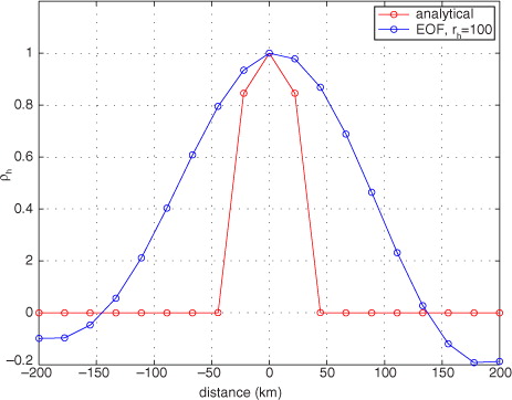
The calculation of the horizontal EOF modes is done on a lower resolution grid, in this setup at 22 km grid resolution, to speed up the computation. The horizontal EOF data are calculated only once and are stored on disk the first time, and can be read very fast in subsequent runs by the data assimilation code. Then the modes are interpolated to the data assimilation grid resolution, which in this case is 11 km. A cross-section of the analytical function in eq. (10) is shown in Fig. 2 along with its EOF counterpart using r _h =100 EOF modes. The figure shows the lower resolution grid, that is, 22 km grid resolution. It is clear that the EOF representation works as intended, but the localization function has in practice become slightly wider than the analytical function due to the limited number of EOF modes. Also, the centre-point value is smaller compared to the analytical function, but in the figure it has been rescaled to be 1.0 in the centre.

Fig. 2 Analytical and EOF approximation of the horizontal localization function. The figure shows a cross-section through the centre point. The number of horizontal EOF modes is 100.

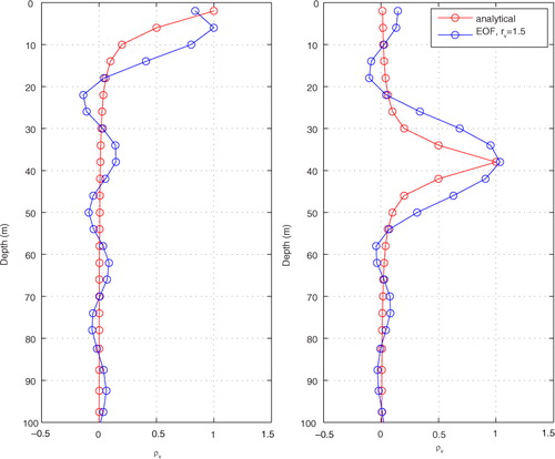
The vertical EOF modes are very fast to calculate on line. So, for simplicity, they are not stored on disk but recalculated each time they are needed, that is, once for each data assimilation cycle. Figure 3 shows the shape of the vertical localization function, with examples from the two vertical levels 1 and 10 as a reference (2 and 38 m depth, respectively), and how big the damping of adjacent layers becomes. The EOF representations of the functions have a maximum slightly smaller than unity, but in the figure it has been rescaled to be 1.0 as a maximum. The figure shows the result when using r _v =15 vertical EOF modes, which explains 61 % of the variance. This is the number of modes we have chosen to use in this paper. Using r _v =25 vertical EOF modes instead, the analytical function would be even better reproduced with 80 % explained variance. Using r _v =50 vertical EOF modes, we explain 100 % of the variance (i.e. a perfect match), because we only have 50 vertical layers in the model. In contrast, using 100 horizontal EOF modes only explained about 26 % of the variance in the horizontal localization. The reason why so many horizontal modes are required is that we try to represent a very sharp localization function which should be valid over a very large computational domain (see Fig. 1).

Fig. 3 Analytical version and EOF approximation of the vertical localization function for (left panel) level 1 and (right panel) level 10. The number of vertical EOF modes is 15.

Using a larger number of modes helps to keep the EOF approximations closer to the analytical functions, but that increases the computational cost. In fact, the computational time τ of the most time-consuming part of the 3DEnVar code is proportional to r _v , r _h , N and m:17

See Liu et al. (2009) for more discussions on computational costs, especially regarding the introduction of EOFs.

The net result of the localization is that the n×N matrix X _b ^′ is replaced by a 4-D matrix of the size n×N×r _h ×r _v . Similarly, the control vector w in (2), originally of the dimension N×1, is replaced by a 3-D matrix of the size N×r _h ×r _v . Hence, the need for localization increases the computational demands both in terms of computer memory and speed. However, using localization without the EOF approach (or a similar approach), the dimensions of X _b ^′ and w would have been much larger.

3.4. Choosing an ensemble

The success of an ensemble-based data assimilation system depends strongly on the choice of ensemble. A cheap, yet efficient, way of creating an ensemble is to use a few years long free model run. Here, we follow the method of Xie and Zhu (2010) to pick the samples: Depending on the assimilation date, we pick ensemble members from the same season (say, within a 3-month window) from the static ensemble, but for previous years. The free run thus works as a library from which we pick ensemble members. It is not necessary to pick ensemble members every day. Instead, we could choose to use every few days, or make averages over a few days. As we pick ensemble members from the same season as the assimilation date, the ensemble changes slowly over the year, to match the seasons. Hence, even though the library itself is static, the ensemble changes with the seasons.

In the following experiments, we used ensemble data for the period 2006–2011. For each ensemble year, we used a time window of 75 d, centred around the assimilation date, from which we calculated 15 five-day mean values. Hence, with this setup the total number of ensemble members becomes 6×15=90.

As can be seen in eq. (3), the elements of the perturbation matrix X _b ^′ are supposed to be in the form of perturbations from some mean state. However, simply subtracting an arithmetic mean is not a good choice. The reason is that if the time window is long enough, there may very well be a seasonal signal in the ensemble data which should be removed (Oke et al., 2005). This is done in two steps. First, a straight line is fitted using the data from each calendar year. Then the fitted values are subtracted from each calendar day to obtain deviations from the seasonal signal that the straight line represents, and this is then done for all calendar years in the ensemble. Using this procedure, each ensemble member is just a deviation from a low-frequency signal based on the ensemble data.

For a given ensemble, the perturbation matrix X _b ^′ has a certain variability. As the variability will affect the data assimilation increments directly, through eq. (2), it may be necessary to inflate or deflate the variability of X _b ^′ . That is done by multiplying the whole matrix X _b ^′ by an inflation factor. In our case, experiments revealed that good results were obtained from simple tunings of the observation errors while keeping the inflation factor equal to 1.0. However, this is not a general result. Given a certain choice of ensemble, the inflation factor may be considered a tuning parameter and may even be automatically corrected depending on the variance of X _b ^′ (Evensen, 2009).

The elements in the observation error covariance matrix O need to be specified. As stated before, we assume the observation errors to be uncorrelated which implies that the off-diagonal elements are all zero. Hence, we only need to specify the squares of the expected observation errors in the diagonal of O. After some tests, we set the observation error for temperature to 0.50 K, for salinity to 0.25 and for SIC to 0.10, which are all reasonable values. For example, Xie and Zhu (2010) assumed an observation error of 0.50 K near the surface (decreasing with depth), and 0.12 for salinity (also decreasing with depth) in their Pacific experiments, i.e. slightly smaller than in this study. Further, Liu et al. (2013) assumed observation errors of approximately 0.9 K for temperature and 0.09 for salinity. Regarding SIC, Lisaeter et al. (2003) assumed an observation error of 0.05, again slightly smaller than we do here.

The implementation of the 3DEnVar code allows switching on and off the assimilation of (and effect on) all implemented variables. These are SSH, ice variables (for HIROMB: ice concentration, level ice thickness, ridged ice thickness, ridge sail height, ridge density and ice drift components; for NEMO: ice concentration, total ice thickness and ice drift components), salinity, temperature and current velocity components. All variables that are ‘switched on’ are affected by all observations through cross correlations between the variables in the ensemble statistics (the multivariate feature in the implementation), so care must be taken before switching on, for example, SSH when assimilating other variables unless previous tests have shown a benefit from this. In this paper, the following variables were included in the data assimilation (including cross correlations): (1) SIC, (2) level ice thickness, (3) temperature and (4) salinity. Assimilation of surface currents from HF radars has also recently been tested in short experiments with good results using the 3DEnVar system, but those results will be reported elsewhere. Furthermore, assimilation of sea level anomalies will also be tested in the future.

4. Results

4.1. Single-surface observations of salinity and temperature

To test the assimilation system we will start by making experiments similar to so-called single-observation experiments. The difference is that we will use six observations at the same time, but distributed in space sufficiently far away from each other. Hence, for a certain region the result would be more or less identical if it had been a single-observation experiment. The benefit of assimilating more than one at a time in this way is simply that it lets us see the effect of single observations in many regions at the same time on a single map.

We will start with salinity. The first-guess field is from a real simulation, valid at 00 UTC on 4 January 2011, but the observations are synthetic and chosen to have values exactly 1.0 above the first guess in each location. The observation locations are chosen from all over the model domain, from the Bothnian Bay, the Bothnian Sea, the Gulf of Finland, the Baltic proper, the Skagerrak and the North Sea (see Fig. 1). The locations are deliberately chosen to be near the coast in some cases and further from the coast in other cases. All observations are assumed to be at the surface in this experiment.

Figure 4a shows the result from the experiment in terms of the data assimilation increment δ x. First, we notice that in some locations, in particular in the north, the increment maxima are much smaller than unity, despite the fact that the innovations (observation minus first guess) were exactly +1.0 in all locations. The reason is that in ensemble methods such as 3DEnVar, the increments depend not only on the local innovation, but also on the ensemble statistics (representing the error in the first guess). If the ensemble spread is small in a certain region, the increment will also be relatively small (unless a very small observation error has been assumed). This is the case in the northern test locations, which explains the surprisingly small increments. In the other locations, the variability in surface salinity is higher, resulting in increments much closer to unity. At the six observation locations, the increments are in the range +0.41 to +1.00.

Fig. 4 Result from assimilating six synthetic observations of (a) SSS and (b) SST. The observation locations are indicated with crosses (+).

The next thing we may notice is that the structures of the increments are rather non-isotropic. The reason is that persistent local currents (e.g. near a coast) affect the ensemble statistics in a way that the increment structures often seem to follow coasts and form ellipses, for example, the location in the North Sea. Surprisingly, the structures in the Baltic proper location are also elongated, despite the relatively long distance to the coast. This may be due to recurring current directions in this area.

Next, we will make a similar experiment but with SST instead. The observation locations are identical to the salinity experiment and the innovations (observation minus first guess) were chosen to be exactly +1.0 °C. The result in terms of assimilation increment is shown in Fig. 4b. In this case, the values in the local maxima of the increments have a smaller spread, in the range +0.96 to +1.00 °C. The difference to the salinity experiment in this respect is that the variability of SST is much larger. In addition, we see that the regions affected by each observation are larger in the temperature experiment compared with the salinity experiment. The interpretation is that the horizontal correlation length scales are larger for temperature in this region. Regarding the shapes of the structures, we see an ellipse-shaped structure in the Gulf of Finland, whereas in the central Baltic proper we see a more circular shape. Summarizing the differences between the surface salinity and temperature experiments, there is a tendency for smaller length scales and more elliptical structures for the salinity increments compared with the temperature increments.

The horizontal localization should ideally suppress all long-distance correlation, but we see some non-zero features away from the observation locations. This is because we only use a limited number of horizontal EOF modes. However, the amplitudes of these long-range structures are probably small enough not to give us any problems, otherwise we need to increase the number of horizontal EOF modes which increases the computational cost.

4.2. Assimilation of SST

Now it is time to test the data assimilation with real observations. We choose an analysed SST field from the Swedish Ice Service at SMHI produced using the so-called IceMap system (digitized data based on hand-drawn charts), valid at 00 UTC on 4 January 1989. The SST data set had a resolution of 11 km.

Figure 5a shows the innovation field (observation minus first guess) in each observation point, which reveals that the first-guess field was too warm except in the Kattegat–Skagerrak region and the south-western part of the Baltic proper. Comparing the innovation with the data assimilation increment in Fig. 5b we see many similarities, even in the details. The signs of the innovation and the increment are in general the same, and so are the magnitudes. In fact, the increment field is almost a perfect copy of the innovation field, only slightly smoothed and having slightly smaller amplitude, as expected. The smooth data assimilation increment field in Fig. 5b is a result of overlapping BECs and localization functions. Nevertheless, it has certain horizontal structures, for example, cooling along the eastern Bothnian Sea and the southern Baltic proper and in the central Kattegat, whereas there is warming in the south-western Baltic proper, the Danish straits and the Skagerrak.

Fig. 5 Experiment of assimilating a real SST field, in terms of (a) innovation, (b) assimilation increment, and (c) observations and (d) analysis.

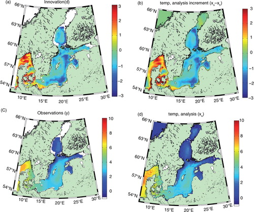
Panels (c) and (d) in Fig. 5 show the observed SST field and the resulting analysis SST field, respectively. We see that many small-scale features in the first-guess field (not shown) have survived and are still present in the analysis in Fig. 5d, e.g. in the Skagerrak and the southern Baltic proper.

4.3. Assimilation of SIC

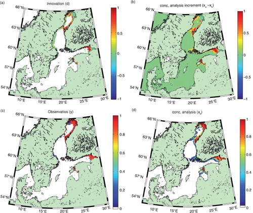
Next we will make an experiment in which we assimilate a real SIC field. The data is again from the IceMap system, just like the SST data above, and also valid on 4 January 1989. Again, the first guess field is from a free model run without data assimilation, valid on the same date. The SIC data had a resolution of 5.5 km.

Figure 6a shows the SIC innovation field, which reveals that the first guess had too little ice in the Bothnian Bay and the Gulf of Finland. The increment field in panel (b) shows a good correspondence with the innovation field, but as expected the increment field is smoother and slightly damped. The analysis field in panel (d) reveals some noise in terms of small regions having non-zero ice concentration values, e.g. in the central Bothnian Bay, where we expect open water. Comparing with the observation field in panel (c) we understand that the noise is a result of the data assimilation itself and is due to the fact that even small levels of noise in the increment field, result in small but positive ice concentration values in the analysis. Some additional noise has already been removed artificially by comparing with the SST field and assuming a threshold value of SST (here set to +1 °C) above which SIC and other ice variables are set to zero.

Fig. 6 Experiment of assimilating a real SIC field, in terms of (a) innovation, (b) assimilation increment, and (c) observations and (d) analysis.

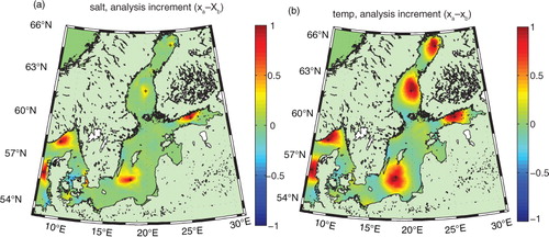
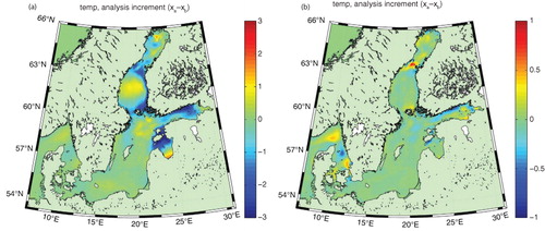
It is also interesting to see how other variables have changed during the process of assimilating SIC data. Remember, the 3DEnVar system as it is implemented here is multivariate, which implies that many variables are affected simultaneously. The SST increment in Fig. 7a reveals that almost everywhere where the data assimilation adds ice, the SST decreases as could be expected. This is physically sound and is a direct result of the covariances between temperature and ice concentration in the ensemble used here. This helps keeping the ice–ocean model from regenerating ice immediately where we just removed it through data assimilation. However, the SST increments are rather large and negative in some places. This could potentially lead to problems, depending on how the ice thermodynamics in the circulation model works. In HIROMB, any negative heat content (relative to the freezing temperature) is converted to equivalent ice volume. Hence, this needs to be checked in longer reanalysis runs. Figure 7b shows the corresponding SSS increments, which are rather small (less than 1) and of varying signs. However, as the salinity is of the order of 1 near some river mouths, the circulation model must be able to keep the salinity from becoming negative, artificially if needed.

Fig. 7 Changes in (a) SST and (b) SSS as a result of assimilating SIC.

4.4. Deep single-observation experiments: salinity and temperature

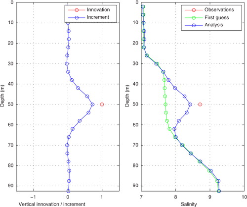
So far we have only considered the 2-D ocean surface. In a reanalysis system it is also important to be able to assimilate vertical profiles of salinity and temperature. The test location was 50 m depth at the standard measuring station BY5 (see the map in Fig. 1), located at 55 °15′ N, 15 °59′ E. The first-guess field was from 25 January 1989.

A synthetic observation with a salinity exactly 1.0 above the first guess was used. The result is shown in Fig. 8. In the left panel we see that the increment profile has a maximum of 0.78 and that the profile is very smooth. The increment is halved about 5 m above and below the observation depth, and at a vertical distance of 15 m the increment is practically zero. The right panel in Fig. 8 shows the resulting salinity profile. The profile looks unrealistic as it is unstable, but this is just a test of the assimilation properties.

Fig. 8 The result of a single-observation experiment for salinity at 50 m depth with an innovation of +1.0.

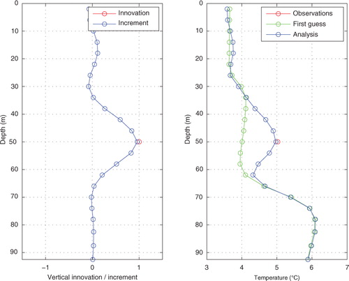
The corresponding temperature experiment, with a synthetic observation exactly 1.0 °C above the first guess, is shown in Fig. 9. In the left panel we see that the maximum increment is +0.96 °C. The increment profile is slightly broader than in the salinity case, but otherwise very similar. The right panel in Fig. 9 shows the end result, with a clear change in temperature near 50 m depth.

Fig. 9 The result of a single-observation experiment for temperature at 50 m depth with an innovation of +1.0 °C.

4.5. Assimilation of real salinity and temperature profiles

Now it is time to test real, observed salinity and temperature profiles, both made at station BY5 (see the map in Fig. 1). The observations and first-guess fields were both from 25 January 1989.

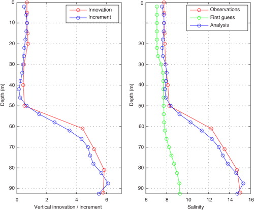
The result from the salinity profile experiment is shown in Fig. 10. The left panel shows the innovation as well as the increment, and the right panel shows the observations, the first guess and the analysis. We see that in this experiment the first guess slightly underestimates the salinity in the surface layer, and grossly underestimates it in the deep layer to the extent that the two-layer structure is almost absent (see the ‘First guess’ in Fig. 10). The data assimilation succeeds in improving the model field to a very high degree. The profile changes from an almost linear stratification to a two-layer structure, as observed. The bottom salinity becomes very close to the observed value, about 15. The increment profile is rather successful in the sense that it mimics the innovation profile, even though there is a slight overshooting at 50 m depth. This may be due to overlapping correlation and localization functions, i.e. contributions from observations at other levels, or possibly to oscillations in the EOF representation of the horizontal localization function.

Fig. 10 Experiment of assimilating a real salinity profile. The left panel shows the innovation profile and the resulting increment profile, and the right panel shows the observations, the first guess and the results of the assimilation.

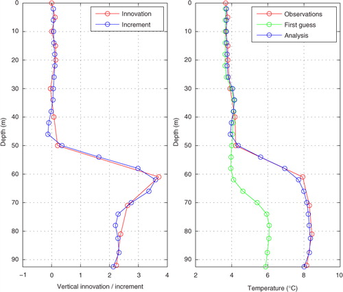
The corresponding results from the temperature profile experiment are shown in Fig. 11. We see that the innovation profile changes sign in the upper half of the water column, and that the increment does not always have the correct sign. The values of the innovations and the increments are rather small, however, so the errors are also small. In the bottom layer, the increments are larger, almost +4 °C at the maximum, and the increment profile manages to mimic the shape rather well, also in terms of magnitude.

Fig. 11 Experiment of assimilating a real-temperature profile. The left panel shows the innovation profile and the resulting increment profile, and the right panel shows the observations, the first guess and the results of the assimilation.

4.6. Sanity test of the system in a 25-yr reanalysis test run

Finally we tested the system (circulation model + 3DEnVar) in a longer test run. We simulated the 25-yr period January 1989 to December 2013, both with and without data assimilation (DA). Instead of spinning up the model before the start, the initial condition was taken from an earlier simulation valid on January 1st of the randomly chosen year 2008. The observations used in the assimilated run were SST, SIC and SIT (Sea Ice Thickness) (all available at least twice a week during Jan–May and December) from the IceMap system, and S/T profiles from the ICES data base (almost daily, but spread out over the domain). Analyses with 3DEnVar were made every 6 hours, which implies a data assimilation window of 6 hours. However, all T/S data for each calendar day were assumed to be valid at 12 UTC, which in practice implies a window length of 24 hours for these variables. SST and ice variables were valid at 00 UTC. The assimilation increments were applied at the first time step in the model. A full documentation of the results of the reanalysis will be published elsewhere, but some results will be shown here.

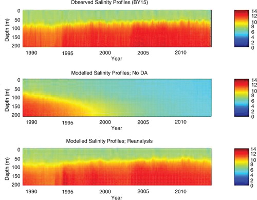
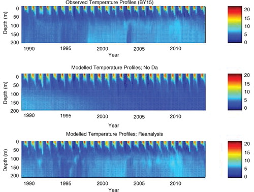
Figure 12 shows the improvement in the vertical salinity structure at station BY15 (see map in Fig. 1), which is representative of the Baltic proper. The observations in panel (a) are the same as used in the data assimilation in the reanalysis, i.e. from the ICES data base. The free run in panel (b) shows how the current setup with HIROMB has great problems with salt-water inflows over longer time scales, which results in almost unstratified water (from a salinity point of view) after about 15 yr. The reanalysis run in panel (c), however, shows how the 3DEnVar data assimilation system is able to maintain the stratification.

Fig. 12 Salinity profiles at station BY15, according to (a) observations, (b) a free run (without data assimilation) and (c) the reanalysis (with data assimilation). The data are sampled once a month.

Figure 13 shows the corresponding result for the vertical temperature structure at BY15 (see map in Fig. 1). The surface layer (upper 50 m) is well simulated by both the free run in panel (b) and in the reanalysis in panel (c), compared to the ICES observations in panel (a). However, the free run has problems with the subsurface layer (below 50 m), due to the lack of deep inflows, whereas the reanalysis run using 3DEnVar shows a much improved result. Similar results (not shown) are found in other subbasins, for both salinity and temperature.

Fig. 13 Temperature profiles at station BY15, according to (a) observations, (b) a free run (without data assimilation) and (c) the reanalysis (with data assimilation). The data are sampled once a month.

The above results were obtained using dependent observations, i.e. the same observations that were used in the data assimilation (from the ICES data base) are used for the verification. There is another data base called SHARK (Svenskt Havsarkiv, or Swedish Ocean Archive), maintained by SMHI, which also contains in-situ observations. ICES and SHARK overlap to a high degree, but with an automatic search algorithm it was possible to find observations in the SHARK data base that were not present in the ICES data base. These observations were thus independent as they had not been used in the reanalysis and could therefore be used to calculate error statistics. The data were from the Baltic Sea only and spread over time and space. The observation operator in the 3DEnVar code was used to interpolate from model space to observation space for each available independent observation, for the free run (‘No DA’) as well as for the reanalysis (‘With DA’).

The results are shown in Fig. 14 in terms of annual mean values of bias errors and as rms errors. We see in panel (a) that in the surface layer (0–50 m deep), both the bias errors and the rms errors were reduced in the reanalysis compared to the free run, for almost all years. In the deeper layers (50–500 m), the improvement is even larger; see panel (b).

Fig. 14 Bias and rms errors from two 25-yr simulations, a free simulation (‘No DA’) and a reanalysis run (‘With DA’). The panels show (a) near-surface salinity (0–50 m), (b) subsurface salinity (50–500 m), (c) near-surface temperature (0–50 m) and (d) subsurface temperature (50–500 m).

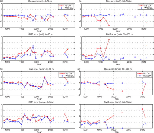
The results for temperature in the surface layer are shown in Fig. 14c, which indicates that the bias errors and rms errors are only slightly reduced in the reanalysis compared to the free run, whereas in the deeper layers the errors are greatly reduced; see panel (d).

For SSH, the results were almost identical between the free run and the reanalysis experiment and rather good compared to coastal tidal gauges (not shown). For ice variables (not shown), some noise (as discussed above) was sometimes detected which tended to deteriorate the results in some situations.

5. Summary and discussion

The 4DEnVar data assimilation system for meteorological data assimilation described by Liu et al. (2008) and Liu et al. (2009) has been implemented in a 3-D form (3DEnVar) for ocean and sea ice data assimilation. It has been adapted for use with the ocean circulation models HIROMB (e.g. Funkquist and Kleine, 2007; Axell, 2013) and NEMO (Madec and the NEMO team, 2008), which are both run at SMHI today. In this paper we chose to use HIROMB as the circulation model.

The data assimilation system relies on ensemble statistics from previous model runs, and the result is very much dependent on that statistics. A semi-static ensemble was used (Xie and Zhu, 2010), based on a 6-yr free model run and 5-day mean values calculated from a time window of 75 d centred around the assimilation window, which results in 90 ensemble members.

To avoid spurious long-range correlations, horizontal and vertical localization was applied. The length scale of the former was chosen to be 50 km and the latter to one vertical grid cell unit, or about 4 m near the surface. Due to the use of a limited number of horizontal EOF modes in the localization implementation, the length scales were in practice somewhat larger than this, however. If smaller length scales should be used in the future, more EOF modes must be used which increases the computational costs.

The results from surface experiments showed that SST had relatively long BEC length scales in the tested region, at least of the order of 100 km. In contrast, SSS had much shorter BEC length scales in the same region, less than 25 km (except along coasts). The results were realistic for both temperature and salinity. It was found that near the coasts the assimilation structure functions tended to be oriented along the coast, especially for salinity. In the open ocean, salinity also had somewhat elongated structures, whereas temperature had more isotropic structures.

The experiments with real SST and SIC fields also gave realistic results. Rather smooth increment fields were produced, and the increment fields changed sign whenever the innovation field changed sign, as far as can be expected. The analysis fields looked realistic, except for some noise in the SIC field for concentrations close to zero; see Fig. 6d.

This problem has many reasons. First, the noise seems to occur in regions where the innovation field is zero. Very close to observation locations, we should expect non-zero increments due to the BEC length scales for SIC. If these length scales are too long due to bad ensemble statistics, the increments should be dampened by the horizontal localization. However, in this case it seems that this is not enough. The SIC values in the analysis are very small, however, so the problem may not be so large in terms of heat in the ocean. To make the localization more efficient, we must increase the number of horizontal EOF modes, but we are already using 100 modes which is very expensive.

Second, the problem is partly related to the fact that SIC does not have a Gaussian distribution. Rather, it is bimodal as it is constrained by Nature to be in the range 0–1 (0–100 %), in many locations often resulting in SIC values close to either zero or one. The problem arises in locations where we initially have SST above the freezing point, and hence zero SIC. Small positive increments in SIC in these locations result in positive SIC in the analysis, even though the SST is above the freezing point. Hence, it is the incremental approach we are using in the data assimilation (where we add an increment to a first guess) that is failing in this case. The reason is that SST and SIC are strongly linked to each other and should perhaps not be treated separately as we are doing here.

One possible way to solve the problem would be to assimilate the heat content of the ocean instead. Given a certain surface water temperature and a certain sea ice volume, we can easily calculate the heat content, both for model data and for observations (if we have observations or estimates of the ice thickness as well). After the assimilation step we need to calculate the ice thickness and concentration from a heat deficit, which is not trivial due to an ambiguity. A certain ice volume could be either in the form of thin ice covering the whole grid cell, or rather thick ice covering only part of the grid cell. Despite expected problems with this ambiguity, this assimilation approach for sea ice should be investigated in the future.

Another obvious approach to improve the ice data assimilation would be to improve the ensemble. In these experiments we used ensemble members from a historical simulation and picked members from the same season as the analysis. A better choice would be to use ensemble members from a real ensemble forecast, in which all members are valid at the analysis time. This approach would probably reduce the problems with the near-surface data assimilation, including SST and SSS. This is an obvious candidate to test in future experiments.

The assimilation of the salinity and temperature profiles gave realistic results in the test location BY5. This is a rather active area with lots of variability, both in Nature and in free model runs (and hence in X _b ^′ ). In other regions (or seasons) where the variability is smaller, we have seen worse results (not shown here) with rather small increments.

It should be noted that as X _b ^′ represents the spread of the ensemble, it is implicitly assumed that it is related to the uncertainty in the first guess (the background error). Hence, if X _b ^′ is small in a certain region, for a certain variable, we also assume the background error is small here, and vice versa. For each location, it is the ratio between the observation error and the model error which is important, together with the innovations (observations minus the first guess in observation space).

If the ensemble spread is too small it is difficult to update the model correctly, because the assimilation system interprets this as relatively small errors in the first guess. This is a dilemma and an important problem to solve in the future. On the one hand, small perturbations in the ensemble statistics means we are relatively confident that the first guess has small errors and that we should not let observations with large innovations ruin the analysis. In this respect, it is only natural that the data assimilation system gives only a small increment. On the other hand, it is often the case that oceanographic models underestimate the variability due to limitations in the physics and resolution, which may also result in biases. How should we correct these biases if the assimilation system is confident the errors in the first guess are small? One way forward could be to artificially increase the variability (in X _b ^′ ) in certain regions, to allow for larger assimilation increments. This can be justified from the point of view that the model error is often larger than the ensemble spread indicates. This method of inflating the ensemble spread for certain depth levels has been tested by the present authors, with some success in the sense that it works from a technical point of view, but not in longer simulations.

Above we suggested to use an ensemble based on an ensemble forecast to improve the data assimilation of surface variables. Unfortunately, that kind of ensemble would likely fail for deep T/S profiles. The reason is that the ensemble spread in deep layers from such a forecast is much too small to be representative of forecast background errors, unless specific care is taken to avoid this. So perhaps the best way forward is to use an ensemble based on an ensemble forecast for surface variables (SST, SSS, ice) and an ensemble based on a historic free run (like the one used in this paper) for T/S profiles.

Nevertheless, the 25-yr test of the system gave reasonable results and the conclusion is that the 3DEnVar data assimilation method can indeed be used in both reanalysis work and operational forecasting. However, the problem of finding an ensemble of model runs (to calculate ensemble statistics from) which is perfect in all respects should not be underestimated. In the future, the task of creating an improved ensemble will be revisited.

6. Acknowledgements

Financial support from the Swedish–Finnish Winter Navigation Board, project VARICE (contract TRAFI/12261/ 02.03.01/2011) and the EU-funded projects MyOcean2 (contract FP7-SPACE-20011-1) and Copernicus (contract no 2015/S 009-011266) are gratefully acknowledged. The in situ T/S data were extracted from the ICES oceanographic data base (http://www.ices.dk/) and is gratefully acknowledged. We also thank three anonymous reviewers for constructive criticism.

References

- Alenius P. , Nekrasov A. , Myrberg K . Variability of the baroclinic Rossby radius in the Gulf of Finland. Cont. Shelf. Res. 2003; 23(6): 563–573.
- Arheimer B., Dahné J., Lindström G., Strömqvist J. Water and nutrient simulations using the HYPE model for Sweden vs. the Baltic Sea basin – influence of input data quality and scale. Hydrol. Res. 2012; 43: 315–329. DOI: http://dx.doi.org/10.2166/nh.2012.010.
- Axell L.B. Wind-driven internal waves and Langmuir circulations in a numerical ocean model of the southern Baltic Sea. J. Geophys. Res. 2002; 107(C11): 3204,. DOI: http://dx.doi.org/10.1029/2001JC000922.
- Axell L . BSRA-15: A Baltic Sea Reanalysis 1990–2004. 2013; Norrköping, Sweden: Swedish Meteorological and Hydrological Institute. Reports Oceanography, 45.
- Buehner M . Ensemble-derived stationary and flow-dependent background-error covariances: evaluation in a quasi-operational NWP setting. Q. J. R. Meteor. Soc. 2005; 131: 1013–1043.
- Buehner M. , Houtekamer P. , Charette C. , Mitchell H. , He B . Intercomparison of variational data assimilation and the ensemble Kalman filter for global deterministic NWP. Part I: description and single-observation experiments. Mon. Wea. Rev. 2010a; 138: 1550–1566.
- Buehner M. , Houtekamer P. , Charette C. , Mitchell H. , He B . Intercomparison of variational data assimilation and the ensemble Kalman filter for global deterministic NWP. Part II: one-month experiments with real observations. Mon. Wea. Rev. 2010b; 138: 1567–1586.
- Compo G. P., Whitaker J. S., Sardeshmukh P. D., Matsui N., Allan R. J., co-authors. The twentieth century reanalysis project. Q. J. R. Meteor. Soc. 2011; 137: 1–28. DOI: http://dx.doi.org/10.1002/qj.776.
- Counillon F. , Bertino L . Ensemble optimal interpolation: multivariate properties in the Gulf of Mexico. Tellus A. 2009; 61: 296–308.
- Courtier P. , Andersson E. , Heckley W. , Pailleux J. , Vasiljevic D. , co-authors . The ECMWF implementation of three-dimensional variational assimilation (3DVAR). I:Formulation. Q. J. R. Meteor. Soc. 1998; 124: 1783–1807.
- Dahlgren P., Kållberg P., Landelius T., Undén P. EURO4M Project – Report, D 2.9 Comparison of the Regional Reanalyses Products with Newly Developed and Existing State-of-the Art Systems. 2014. Technical Report. Online at: http://www.euro4m.eu/Deliverables.html.
- Daley R . Cambridge Atmospheric and Space Sciences Series. Atmospheric Data Analysis. 1991; Cambridge University Press. Chap. 3.
- Dee D. P. , Uppala S. M. , Simmons A.J. , Berrisford P. , Poli P. , co-authors . The ERA-Interim reanalysis: configuration and performance of the data assimilation system. Q. J. R. Meteorol. Soc. 2011; 137: 553–597.
- Ebita A. , Kobayashi S. , Ota Y. , Moriya M. , Kumabe R. , co-authors . The Japanese 55-year Reanalysis ‘JRA-55’: an interim report. SOLA. 2011; 7: 149–152.
- Evensen G . Sequential data assimilation with a nonlinear quasi-geostrophic model using Monte Carlo methods to forecast error statistics. J. Geophys. Res. 1994; 99: 143–162.
- Evensen G . The ensemble Kalman filter: theoretical formulation and practical implementation. Ocean Dyn. 2003; 53: 343–367.
- Evensen G . Data assimilation: the ensemble Kalman Filter. 2009. Springer-Verlag, Heidelberg, Germany.
- Fisher M. , Courtier P . Estimating the covariance matrices of analysis and forecast error in variational data assimilation. ECMWF Tech. Memo .
- Fu W. , She J. , Dobrynin M . A 20-year reanalysis experiment in the Baltic Sea using three-dimensional variational (3DVAR) method. Ocean Sci. 2012; 8: 827–844.
- Funkquist L. , Kleine E . Report Oceanography, 37. HIROMB: An Introduction to HIROMB, an Operational Baroclinic Model for the Baltic Sea. 2007; Norrköping, Sweden: Swedish Meteorological and Hydrological Institute.
- Gibson J. , Kållberg P. , Uppala S. , Hernandez A. , Nomura A. , co-authors . ERA Description. Re-Analysis (ERA) Project Report Series 1, ECMWF. 1997. European Centre for Medium-Range Weather Forecasts, Reading, Great Britain.
- Gustafsson N . Discussion on ‘4D-Var or EnKF’. Tellus A. 2007; 59: 774–777.
- Gustafsson N. , Berre L. , Hornquist S. , Huang X.-Y. , Lindskog M. , co-authors . Three-dimensional variational data assimilation for a limited area model. Part I: general formulation and the background error constraint. Tellus A. 2001; 53: 425–446.
- Gustafsson N, Bojarova J. Four-dimensional ensemble variational (4D-En-Var) data assimilation for the HIgh Resolution Limited Area Model (HIRLAM). Nonlin. Process. Geophys. 2014; 21: 1–18. DOI: http://dx.doi.org/10.5194/npg-21-1-2014.
- Gustafsson N., Bojarova J., Vignes O. A hybrid variational ensemble data assimilation for the HIgh Resolution Limited Area Model (HIRLAM). Nonlin. Process. Geophys. 2014; 21: 303–323. DOI: http://dx.doi.org/10.5194/npg-21-303-2014.
- Hamill T. , Snyder C . A hybrid ensemble Kalman filter-3D variational analysis scheme. Mon. Wea. Rev. 2000; 135: 222–227.
- Hamill T. , Snyder C. , Morss R . Analysis-error statistics of a quasigeostrophic model using three-dimensional variational assimilation. Mon. Wea. Rev. 2002; 130: 2777–2790.
- Houtekamer P. , Mitchell H . A sequential ensemble Kalman filter for atmospheric data assimilation. Mon. Wea. Rev. 2001; 129: 123–137.
- Kalnay E. , Kanamitsu M. , Kistler R. , Collins W. , Deaven D. , co-authors . The NCEP/NCAR 40-year reanalysis project. Bull. Amer. Meteor. Soc. 1996; 77: 437–471.
- Leppäranta M. , Myrberg K . Physical Oceanography of the Baltic Sea. 2009. Springer-Verlag, Heidelberg, Germany.
- Lisaeter K. A. , Rosanov J. , Evensen G . Assimilation of ice concentration in a coupled ice–ocean model, using the Ensemble Kalman filter. Ocean Dyn. 2003; 53: 368–388.
- Liu C. , Xiao Q . An ensemble-based four-dimensional variational data assimilation scheme. Part III: Antarctic applications with advanced research WRF using real data. Mon. Wea. Rev. 2013; 141: 2721–2739.
- Liu C. , Xiao Q. , Wang B . An ensemble-based four-dimensional variational data assimilation scheme. Part I: technical formulation and preliminary test. Mon. Wea. Rev. 2008; 136: 3363–3373.
- Liu C. , Xiao Q. , Wang B . An ensemble-based four-dimensional variational data assimilation scheme. Part II: observing system simulation experiments with Advanced Research WRF (ARW). Mon. Wea. Rev. 2009; 137: 1687–1702.
- Liu Y. , Meier M. , Axell L . Reanalyzing temperature and salinity on decadal time scales using the ensemble optimal interpolation data assimilation method and a 3D ocean circulation model of the Baltic Sea. J. Geophys. Res. 2013; 118: 5536–5554.
- Lorenc A . The potential of the ensemble Kalman filter for NWP – a comparison with 4D-Var. Q. J. R. Meteorol. Soc. 2003; 129: 3183–3203.
- Luhamaa A. , Kimmel K. , Männik A. , R[otilde][otilde]m R . High resolution re-analysis for the Baltic Sea region during 1965–2005 period. Clim. Dyn. 2011; 36: 727–738.
- Madec G. , The NEMO Team . NEMO Ocean Engine. Note du Pole de modelisation. 2008. 27. Institut Pierre-Simon Laplace (IPSL), France. ISSN No. 1288-1619.
- Nerger L. , Hiller W. , Schrter J . A comparison of error subspace Kalman filters. Tellus A. 2005; 57: 715–735.
- Oke P., Allen J., Miller R., Egbert G., Kosro P. Assimilation of surface velocity data into a primitive equation coastal ocean model. J. Geophys. Res. 2002; 107: 3122. DOI: http://dx.doi.org/10.1029/2000JC000511.
- Oke P. , Schiller A. , Griffin D. , Brassington G . Ensemble data assimilation for an eddy-resolving ocean model of the Australian region. Q. J. R. Meteorol. Soc. 2005; 131: 3301–3311.
- Omstedt A. , Axell L.-B . Modeling the seasonal, interannual, and long-term variations of salinity and temperature in the Baltic proper. Tellus A. 1998; 50: 637–652.
- Onogi K. , Tsutsui J. , Koide H. , Sakamoto M. , Kobayashi S. , co-authors . The JRA-25 Reanalysis. J. Meteor. Soc. Japan. 2007; 85: 369–432.
- Osinski R. , Rak D. , Walczowski W. , Piechura J . Baroclinic Rossby radius of deformation in the southern Baltic Sea. Oceanologia. 2010; 52(3): 417–429.
- Parrish D. , Derber J . The National Meteorological Center's spectral statistical interpolation analysis system. Mon. Wea. Rev. 1992; 120: 1747–1763.
- Pham D. , Verron J. , Roubaud M . A singular evolutive extended Kalman filter for data assimilation. J. Mar. Syst. 1998; 16: 323–340.
- Umlauf L. , Burchard H. , Hutter K . Extending the k - w turbulence model towards oceanic applications. Oc. Mod. 2003; 5: 195–218.
- Uppala S. M., Kållberg P. W., Simmons A.J., Andrae U., Da Costa Bechtold V., co-authors. The ERA-40 re-analysis. Q. J. R. Meteorol. Soc. 2005; 131: 2961–3012. DOI: http://dx.doi.org/10.1256/qj.04.176.
- Wang K. , Leppäranta M. , Gästgivars M. , Vainio J. , Wang C . The drift and spreading of the Runner 4 oil spill and the ice conditions in the Gulf of Finland, winter 2006. Estonian J. Earth Sci. 2008; 57(3): 181–191.
- Wang X. , Bishop C . A comparison of breeding and ensemble transform Kalman filter ensemble forecast schemes. J. Atmos. Sci. 2003; 60: 1140–1158.
- Wang X. , Lei T . GSI-based four-dimensional ensemble-variational (4DEnsVar) data assimilation: formulation and single-resolution experiments with real data for NCEP global forecast system. Mon. Wea. Rev. 2014; 142: 3303–3325.
- Wilcox D . Turbulence Modeling for CFD. 1998; Inc: DCW Industries. 2nd ed.
- Wilhelmsson T . Licentiate Thesis. Parallellization of the HIROMB Ocean Model. 2002. Royal Institute of Technology, Department of Numerical and Computer Science, Stockholm, Sweden.
- Xie J. , Zhu J . Ensemble optimal interpolation schemes for assimilating Argo profiles into a hybrid coordinate ocean model. Ocean Model. 2010; 33: 283–298.
- Zhang H. , Xue J. , Zhuang S. , Zhu G. , Zhu Z . GRAPeS 3D-Var data assimilation system ideal experiments. Acta Meteor. Sin. 2004; 62: 31–41.