Ensemble-based approximation of observation impact using an observation-based verification metric

Abstract

Knowledge on the contribution of observations to forecast accuracy is crucial for the refinement of observing and data assimilation systems. Several recent publications highlighted the benefits of efficiently approximating this observation impact using adjoint methods or ensembles. This study proposes a modification of an existing method for computing observation impact in an ensemble-based data assimilation and forecasting system and applies the method to a pre-operational, convective-scale regional modelling environment. Instead of the analysis, the modified approach uses observation-based verification metrics to mitigate the effect of correlation between the forecast and its verification norm. Furthermore, a peculiar property in the distribution of individual observation impact values is used to define a reliability indicator for the accuracy of the impact approximation. Applying this method to a 3-day test period shows that a well-defined observation impact value can be approximated for most observation types and the reliability indicator successfully depicts where results are not significant.

• data assimilation
• forecast sensitivity to observations
• FSO

1. Introduction

Maintaining an operational observing network is an intricate and expensive task. It is therefore essential to evaluate the contribution of various components of the network and potential new observing systems to forecast accuracy. This contribution, traditionally referred to as observation impact, can in principle be evaluated by parallel numerical data denial experiments, often named observing systems experiment (OSEs) (e.g. Harnisch et al., 2011; Weissmann et al., 2011). Given the computational expense of such experiments, however, this approach is only feasible for few configurations of an observing network and limited periods. In view of an operational observation impact assessment, it is therefore desirable to approximate the impact efficiently without additional numerical experiments.

The first approximation method emerged in the framework of developing adjoint models and four-dimensional variational data assimilation systems: Baker and Daley (2000) described a method of propagating the forecast sensitivity to the observations (FSO), building upon earlier research that developed the sensitivity of a forecast aspect (error) to the analysis (Langland and Rohaly, 1996). Langland and Baker (2004) linked this FSO to the impact of observations and by this performed the last step for the adjoint approximation of the forecast impact of observations (referred to as forecast sensitivity observation impact or FSOI). Building upon these developments, several studies calculated the FSOI to assess the contribution of components of the operational observing network (Langland, 2005; Cardinali, 2009; Gelaro et al., 2010; Baker et al., 2014) or special field campaign observations (Weissmann et al., 2012). A systematical comparison of FSOI with data denial results can be found in Gelaro and Zhu (2009).

More recently, an analogous to the FSOI method has been proposed by Liu and Kalnay (2008), Li et al. (2010) and Kalnay et al. (2012) for ensemble data assimilation systems, specifically for a Localised Ensemble Transform Kalman Filter (LETKF). In support of the notation FSOI for the adjoint-based approximation of observation impact, the ensemble-based approximation could be named as EnFSOI. Ota et al. (2013) applied the EnFSOI to assess the impact of the components of the global observing network and Kunii et al. (2012) to evaluate the impact of observations on tropical cyclone forecasts. Sommer and Weissmann (2014) first applied the method in a convective-scale modelling environment and demonstrated that the approximated impact agrees reasonably well with parallel numerical (data denial) experiments.

All studies mentioned above used later analyses for the quantification of forecast error and its reduction by observations. In both, the adjoint and the ensemble approach, the approximation is limited to comparably short lead times (about 12–24 hours on the global scales and 3–6 hours on the convective scale) due to underlying linearity assumptions. For these lead times, however, the later analysis is still highly correlated with the forecast as information is cycled to later analyses through the use of a short-range forecast as first-guess in the data assimilation procedure. Cardinali et al. (2004), for example, estimated that the influence of the first-guess on the subsequent analysis is about 85 %, whereas all assimilated observations only contribute 15 % of the information in a 12-hour window 4D-Var assimilation system (Rabier et al., 2000). In contrast, later observations can always provide an independent verification (for observing systems that are not assimilated) or a comparably independent verification (for observing systems that are assimilated).

A further limitation of the impact approximation is that it works reliably on a statistical basis, but not necessarily for a single observation or a small group of observations in a single assimilation cycle. This has been highlighted in several previous studies, but little knowledge exists on the statistical properties of observation impact estimates that determine the reliability of the method, the consequent averaging requirements and lead time limitations. Likely the reliability depends on the observation type, the region, the weather situation and the scales of interest as well as the properties and settings of the data and modelling assimilation system (e.g. ensemble size). To address this case- and system-dependent variation in reliability, it would therefore be advantageous to estimate statistical reliability together with the approximation of observation impact.

The study is outlined as follows: Section 2 describes the approximation and the proposed modification. Section 3 presents results of the observation impact approximation in the convective-scale pre-operational ensemble system of Deutscher Wetterdienst (DWD), discusses statistical properties of observation impact values and derives a reliability indicator to estimate the accuracy of the approximation. Finally, Section 4 provides conclusions of the study.

2. Method

Following Hunt et al. (2007), the LETKF analysis for an ensemble with members at grid point j is computed as:1

As usual, the subscript b stands for a background state (short-term forecast) from a previous analysis, a for an analysis state and f for a forecast to the next analysis time. With this convention, everything below applies to a given analysis time and therefore no time indices are necessary. The following notation is used here:

: Analysis ensemble mean state vector

: Background ensemble mean state vector

: Background ensemble perturbations

: Background ensemble perturbations in observation space

Analysis covariance matrix in ensemble space at grid point j

ρ: Multiplicative inflation parameter

R(j): (Diagonal) observation covariance matrix localized around grid point j

: Observation innovation vector

: Observations

: Ensemble mean of background in observations space

Let d be the vector of all available observation innovation vector and d′ be the innovation vector of a small subset of observations whose impact one is interested in. For notational simplicity, the lengths of d and d′ are made equal, by setting the unobserved components in d′ to zero. In the following, the superscript d stands correspondingly for the set of observations that have been used to compute the analysis or to initialise the forecasts. As in Kalnay et al. (2012), the impact of observations d′ is given by the difference in the respective forecast errors:2

where is the error of the forecast initialised with observations d defined in eq. (3) and the scalar product dot is defined in eq. (4). Contrary to Kalnay et al. (2012), we suggest to use observations (indexed l) for verification instead of the analysis. Verification with observations is seen as a superior approach, since in contrast to the analysis, observations can be expected to be independent or at least comparably independent from the forecast. One limitation of this approach that needs to be kept in mind is that the observational coverage is inhomogeneous in time and space, in particular if only specific observation types are used for verification.

The forecast error is therefore defined relative to the verifying observations3

where H _veri stands for the observation operator into the verification space and the overbar for the ensemble mean. As mentioned before, the superscript stands for the observations that have been used for the initialisation of the forecast. The length of vector is the number of verifying observations. The scalar product in eq. (2) is defined through a metric that includes a normalisation with the observation error and the number of verifying observations N _veri:4

The normalisation with the number of verifying observations is included here to give comparable weight to situations with differing observational density.

The goal is now to find an approximation to eq. (2) that avoids the necessity to compute the forecast error of an experiment neglecting the observations d′. For small d′, J can be approximated by the linearisation around 0:5

Note that J is defined in eq. (2) as a function of the omitted observations. The above expression is therefore not a linearisation around an assimilation with zero observations but rather a linearisation around omitting zero observations from the full set of observations. The first term in eq. (5) vanishes by definition and applying the derivative to the first factor in eq. (2) leaves the second vanishing. Therefore the only remaining expression gives6 7

The last step has been approximated analogously to Kalnay et al. (2012). However, two changes have been applied here:

• Since the aim here is to use observations for verification, the model forecast ensemble has been replaced by its analogue in observation space .

• Instead of approximating first the impact of all available observations d relative to no observations and then deriving the case where some observations are omitted, here we suggest to directly linearise the exact expression [eq. (2)]. The first factor in Kalnay et al. (2012) has thus been corrected to , which is a more accurate approximation. It has also the practical advantage that no forecast initialised without any observations is needed.

Equation (7) only requires quantities that are already computed in the data assimilation and the ensemble forecasting system. It has been implemented in the Km-scale ENsemble Data Assimilation (KENDA, Schraff et al. 2016) system that is currently in development at DWD and in the framework of the Hans-Ertel Centre for Weather Research (HErZ) (Weissmann et al., 2014). KENDA is an implementation of an LETKF combined with the non-hydrostatic limited-area COSMO-DE forecast model (Baldauf et al., 2011) with 2.8 km horizontal grid spacing and 50 vertical levels. The model domain covers approximately 1200×1200 km of central Europe centred over Germany. Boundary conditions were taken from a special 20-member ensemble run of the global model of the European Centre for Medium Range Forecasts (ECMWF) with horizontal resolution increased to T1279 (~16 km). These 20 members were doubled using a time-lagged approach as in Harnisch and Keil (2015). Besides different boundary conditions and an increased ensemble size of 40 members, the experimental set-up used in the present study was largely the same as in Sommer and Weissmann (2014). In the experimental period from 10 June 2012 12 UTC until 13 June 2012 15 UTC, an analysis has been computed every 3 hours which served as the initialisation for a 6 hours forecast. The verification then used all observations in the interval between 3 and 6 hours forecast lead time.

The development of forward operators for the assimilation of remote sensing data in KENDA, for example, for visible and near-infrared satellite reflectance (Kostka et al., 2014), satellite-derived cloud products (Schomburg et al., 2015), global navigation satellite systems (GNSS) total delay or radar reflectivity and radial velocity, is not yet completed. Thus, the present study only assimilates conventional observations consisting of four groups: Temperature and wind observations from aircraft (AIREP), wind profiler observations (PROF), temperature, wind and humidity observations from synoptic surface stations (SYNOP) and temperature, wind and humidity observations from radiosondes (TEMP). Following the standard KENDA set-up at DWD, surface station wind observations were only assimilated in areas with an elevation lower than 100 m as higher orography often causes large representativity errors. As a result, only 17 656 surface station wind observations are assimilated, compared to 61 814 temperature and humidity observations. Surface stations pressure was excluded from the assimilation as it is not fully resolved yet how to localise such integral observations in the vertical. It is clear that this issue needs to be resolved in order to achieve reasonable forecast skill suitable for operational use. In this context, it should also be noted that systematic errors cause a problem for the evaluation of observation impact. However, this is independent of the impact evaluation derived here and work with the pre-operational version of KENDA which includes surface pressure observations is currently ongoing. If not stated otherwise, all assimilated observation types were used also for verification.

As in Sommer and Weissmann (2014), the same localisation is used for the assimilation and the calculation of observation impact (Gaspari-Cohn function with length scales 100 km horizontally and 0.2 ln(p) vertically). Research for more sophisticated localisation methods that consider the propagation of impact with forecast lead time is ongoing (e.g. Gasperoni and Wang 2015), but Sommer and Weissmann (2014) demonstrated that using a static localisation leads to reasonable results for lead times up to 6 hours.

Different concepts exist for quantifying the influence of observations at analysis time, that is, without taking into account the time development. Common methods are degrees of freedom per signal (Wahba et al., 1995), influence matrix diagnostics (Cardinali et al., 2004), analysis sensitivity (Liu et al., 2009) and variance reduction (Brousseau et al., 2013). To obtain a rough estimate of this influence here, the ratio of background error (represented by ensemble spread in observation space) and observation error is computed as an approximation. This ratio determines the weight of observations in the analysis. However, this estimate of observations influence does not account for the spatial distribution of observations; that is, the influence of observations in data-sparse regions is higher than in data-rich regions. The sum of this quantity, evaluated for each observation will be referred to as ‘σ _b /σ _o ’ in the following.

3. Results

3.1. Approximated observation impact

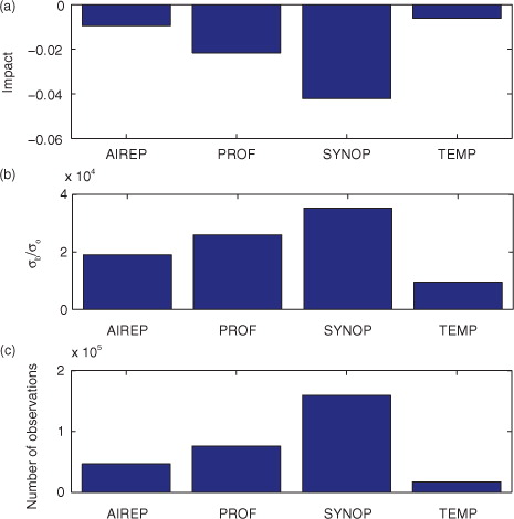
Figure 1(a) shows the approximated observation impact (EnFSOI) of the four observation types computed as described in the previous section accumulated over the 3 d experimental period. All observation types show a negative (i.e. beneficial) impact. Surface stations (SYNOP) exhibit the largest impact followed by wind profilers (PROF), aircraft (AIREP) and radiosondes (TEMP). The impact of different observation types is clearly related to the number of individual observations provided by different systems [Fig. 1(c)] and the corresponding σ _b /σ _o ratio [Fig. 1(b)] approximated as described in Section 2.

Fig. 1 Sums over the 3-days experimental period. (a): Approximated observation impact. (b): σ_b/σ _o . (c): Number of observations. AIREP: Aircraft, PROF: Wind profiler, SYNOP: Surface stations, TEMP: Radiosondes. Verified with all quality-controlled observations between 3 and 6 hours forecast lead time.

The number of observing stations varies considerably between observation types and it is straight forward to compute the impact per observing station. In fact, the comparably expensive wind profiler station has by far the largest impact followed by radiosondes, surface stations and aircraft. The exact relations are shown in Table 1, that is, the number of observations of a given type whose impact equals that of one wind profiler. These numbers could easily be converted to an impact per cost estimate if the expenses of the observing systems were known. For decisions on removing or adding components of the observing system, however, it needs to be kept in mind that observing systems often serve multiple purposes besides numerical weather prediction (e.g. climate monitoring or local forecasting) and that results are very sensitive to the applied verification metric (see Section 3.2). The current configuration with a comparably sparse network of observations for verification to some extent favours temporally continuous observation types (profilers and surface stations) as those always have spatially nearby observations for verification.

Table 1. Number of stations that correspond to one wind profiler in the sense of observation impact

AIREP	SYNOP	TEMP
134	73	16

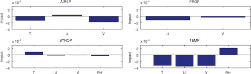
To gain further insights into the contribution of different observation types, Fig. 2 shows the impact of all observation types and variables divided by the respective number of observations. The corresponding approximated σ _b /σ _o ratio is also shown. Radiosonde and surface station temperature observations show the largest impact per individual observation. The impact of radiosonde and aircraft wind components is, on average, slightly smaller than the impact of corresponding temperature observations. Generally, the impact of zonal wind components is clearly higher than that of meridional components, which is not surprising given the location of the model domain in the mid-latitudes with stronger zonal than meridional winds. Surface station temperature observations show a comparably large impact, yet they are not yet assimilated in the pre-operational version of KENDA at DWD (Schraff et al. 2016). This indicates that they are potentially beneficial observations, but quality control routines likely need to be developed for situations with strong surface inversions to assimilate them in an operational context. Radiosonde humidity only shows a very small impact. In this context however, it needs to be mentioned that there are hardly any tropospheric humidity observations in the verification metric and results might change significantly if additional observations of humidity, clouds or precipitation would be included for verification.

Fig. 2 Relative impact of different observed variables: Total impact for each observed variable divided by the respective number of observations and by the impact of all observations. Additionally red bars show the corresponding negative σ _b /σ _o .

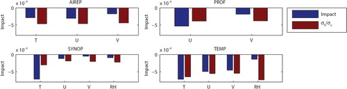
While the total impact per observing system is very similar to the corresponding σ _b /σ _o ratio (Fig. 1), differences of σ _b /σ _o ratio and forecast impact are apparent for some of the variables (Fig. 2). Most strikingly, surface wind observations exhibit a much lower forecast impact than their σ _b /σ _o ratio, which may indicate an imperfect use of the observations in the KENDA system, for example, due to an inappropriate assigned error, imperfect quality control procedures, inappropriate spread of the ensemble at the surface or a potential model bias. The investigation of improved settings for the assimilation of surface observations in KENDA is therefore the focus of subsequent research. Differences are also apparent for surface humidity observations, but, as mentioned above, those may be related to the low weight of humidity in the verification norm. In contrast to the forecast impact, both wind components show a similar σ _b /σ _o ratio and the influence of each wind component is comparable to that of temperature observations for radiosondes and aircraft. Furthermore, the impact of aircraft observations is 2–3 times smaller than that of radiosondes while both systems show a comparable σ _b /σ _o ratio.

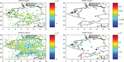
Breaking up the total impact for the individual observing stations results in Fig. 3. For aircraft, the first transmitting location was used. Most stations show a neutral (green) or beneficial (blueish) impact. Overall, the total impact value is dominated by fairly few stations with large negative values. For instance, one wind profiler in the Netherlands, where several showers occurred in the experimental period, contributes most of the total wind profiler impact in the whole period (refer to discussion in 3.3 though). In the same region, several surface stations and one aircraft show a detrimental (reddish) impact. Another systematic feature seems to be a number of surface stations with beneficial (blueish) impact near the northern Alpine rim in southern Germany and northern Switzerland. However, as further discussed in Section 3.3, results summed over only a few observations (here a few 100 per station) are error-prone. It is therefore unclear if for example the detrimental impact of the radiosonde in Payerne, Switzerland, is a meaningful result.

Fig. 3 Total impact summed over the experimental period for each observing station.

3.2. Sensitivity to verification

So far all active observation types in the assimilation have been used for verification but obviously the results can change with a different set of verifying observations. Exemplified, Fig. 4 shows the impact per observation type when verified individually with one of the four observation types. Since each impact value is weighted by the number of verifying observations following eq. (4), the sum of the impact in this figure does not equal Fig. 1(a). As expected, each observation type has the largest impact when verified with the same type and significantly less impact when other types are used for verification. In other words, radiosondes are the best observing system when the forecast is verified against radiosondes and correspondingly for the other observation types. Nevertheless, most observation types also show a beneficial impact when other observation types are used for verification. The only exceptions are the profiler impact verified against surface station and vice versa the surface station impact verified against profilers. This dependence on verification is also a reason why it may be dangerous to actually exclude data that has disadvantageous impact in a specific verification metric; the situation may look different in an other metric.

Fig. 4 Approximated observation impact summed over the experimental period using different observation types for verification.

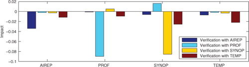
As mentioned before, time-continuous observation types as surface station and profiler are likely favoured in this context as there is always a verifying observation at the same location after 3-h lead time, whereas aircraft are not necessarily at the same location and radiosondes are usually only launched every 12 or 24 hours. While the sensitivity to the verification norm and the inhomogeneity and sparsity of the verification norm needs to be kept in mind, verification with observations is still seen as a superior approach given the correlation of the subsequent analysis with the previous forecast. In particular in the presence of model biases and systematic model deficiencies, the use of analyses for verification is potentially dangerous – particularly if observation impact estimates are actively used for excluding observations through pro-active quality control as proposed by Hotta (2014). Compared to the experimental assimilation system with only conventional observations used in the present study, more advanced systems that also include different types of remote sensing observations can provide a more homogeneous verification. In general, it is desirable to use a verification norm that represents the most complete description of the atmosphere that is available, but caution should be given when including potentially biased or correlated observations as, for example, radiances or atmospheric motion vectors (see e.g. Weissmann et al., 2013). In consequence, the choice of the optimal verification norm may be a trade-off between completeness and reliability provided by independent observations that do not require calibration. Furthermore, a user may prefer to use a verification norm representing a limited set of primary forecast variables (which are often precipitation and surface variables for regional modelling systems).

The previous evaluation used all assimilated observation types for verification and the weight of verifying observations was proportional to their expected errors. Alternatively, a verification norm can be defined that reflects the user quantities of interest (e.g. precipitation, wind gusts and surface temperature) and weighs different variables by the interest for the user or the reliability of the observation type. For example, let J _AIREP ^SYNOP be the impact of surface stations when verified with AIREP and correspondingly for the other groups. To give equal weights to the different verification groups, this can be normalised by the total impact from the AIREP verification: J _AIREP ^SYNOP /J _AIREP ^TOTAL. For the total normalised surface station impact [Jtilde] ^SYNOP, one would then sum over the four verification groups. Introducing weights for the different verification types leads to:8

Table 2 shows the observation impact estimates using different verification norms: (i) all observations as defined in eq. (7); (ii) equal weights of 0.25 for all four observation types; (iii) weights of 0.3 for AIREP/PROF/SYNOP and 0.1 for less frequent radiosonde observations. The latter two norms significantly decrease the dominant impact of surface station observations leading to a fairly similar impact of aircraft, profiler and surface station. Radiosondes still show a lower impact than other observation types and its impact is reduced further when the verification weight for radiosondes is set to 0.1. In this context, it should be noted that the assigned observation error (and thus the weight) in the verification need not be the same as the one in the assimilation.

Table 2. Impact estimates using different verification norms based on eqs. (4) and (7) and surface pressure observations ( J _PS ). Numbers in subscript denote the verification weights α [eq. (8)] for AIREP/PROF/SYNOP/TEMP

Verification norm	AIREP impact	PROF impact	SYNOP impact	TEMP impact
J (7)	11.90 %	27.29 %	53.07 %	7.73 %
(8)	26.72 %	31.09 %	29.70 %	12.49 %
(8)	29.14 %	33.91 %	32.40 %	4.54 %
J PS	36.58 %	−1.35 %	48.74 %	16.03 %

Observational norms can also include quantities that are not assimilated but quality controlled, e. g. surface pressure from synoptic stations, radar observations or integrated water vapour derived from GNSS total delay. An example of results using verification with surface pressure observations is shown in Table 2. Using this norm, the impact estimates are significantly different. Surface stations still exhibit the largest impact, but the impact of radiosondes and aircraft increases, whereas profilers show a slightly detrimental impact. The higher impact of aircraft and radiosondes, particularly by temperature observations of these systems, obviously reflects the direct correlation of the temperature (mass) field with surface pressure. Wind and humidity observations in contrast can only have an indirect effect in this verification norm.

In order to compare results to earlier publications, the approximated impact using a dry total energy metric (Rabier et al. 1996) in model space for verification is shown in Fig. 5. In other words, the error definition eq. (3) is replaced by the difference between the forecast and a new analysis and the norm eq. (4) is replaced by the dry total energy norm. Several features create doubts about the reliability of these results: While it is clear that with the model space based verification metric profile observations like radiosondes (TEMP) may get a higher impact, the value obtained here seems exaggerated. Aircraft show a surprisingly small impact. Furthermore there is a very strong inter-cycle variability, so that the summed impact depends heavily on exactly how many cycles are considered (not shown). The reasons for these issues are likely associated with the strong correlation of the forecast with its verifying analysis.

Fig. 5 Same as figure 2, but using verification in model space.

3.3. Distribution and reliability

Since individual observation impact values exhibit a wide distribution compared to the mean impact of an observation type, it is important to investigate the robustness of results such as the ones shown before. Figure 6 shows semi-logarithmic histograms of all individual observation impact values (green lines). The distribution is obviously highly non-Gaussian and centred around or near zero. The ratio of numbers of negative to positive impact is approximately 48:52, comparable with results of Lorenc and Marriott (2013) and Sommer and Weissmann (2014). It is, however, not only this ratio that determines the total impact but also the amplitude of the individual values. The mean value is very close to zero but still negative (beneficial) for all observation types. The difficulty here is to accurately estimate the mean of a distribution that is very wide compared to the small distance between zero and the mean. It is therefore necessary to check whether it is reliably sampled by the method applied to a 3-day test period.

Fig. 6 Histogram of observation impact values (green) with mean value (red) and fitted stretched exponential (blue).

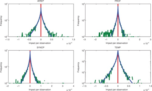
Empirically, one finds that the distributions of impact values in Fig. 6 are well approximated by stretched exponentials of the form

where J is the impact of a single observation and β, γ are parameters to be fitted for positive and negative J separately. This fitted probability distribution is also displayed in Fig. 6 (blue lines). All of these fits are remarkably close to the distribution of impact values – with the exception of negative wind profiler impact values that differ considerably. Assuming the true distribution for a sufficiently large sample size to be a stretched exponential, the deviation from it can serve as a measure for the reliability of the estimate. To this goal, the unfitted total impact (balance point of the area under the green line) is set in relation to the fitted impact (correspondingly for the blue line) (cf Table 3). By doing this, the variability is not taken into account but the interest is to obtain a meaningful measure for the misfit between the two distributions. We propose to use this ratio as a reliability indicator for the estimate. As a suggestion, a ratio lower than 0.8 or higher than 1.2 may be an indication that the true distribution is not well-sampled and a larger sample size (i.e. a longer experimental period) is required for reliable results. Following this, the large value of the ratio of profiler impact and its fitted impact is an indication that these results are not reliable, whereas the ratios for the other three observation types are close to one and indicate reliable estimates. It should be noted that a ‘good’ value of the reliability indicator is only a necessary but not sufficient condition for a reliable estimate.

Table 3. Unfitted impact, fitted impact and their ratio

	AIREP	PROF	SYNOP	TEMP
Unfitted impact	−0.0094491	−0.021665	−0.042126	−0.0061346
Fitted impact	−0.0094963	−0.0095535	−0.042357	−0.0072236
Ratio	0.99503	2.2677	0.99455	0.84924

Another way of addressing this issue is by looking at the cumulative distribution function (CDF) of the individual impact values, that is,9

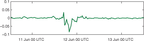
Here, all individual impact values smaller than a given are summed up. The results for the four observation types are shown in Fig. 7. Extreme positive and negative values are very scarce and do not contribute much to the total impact: The curve becomes saturated. The distributions of aircraft, surface stations and radiosondes impact values seem well-sampled in this experiment up to their saturation. In agreement with the results in Table 3, we therefore expect the results to be reliable estimates. For wind profilers, few, but large negative values cause a difference between the experimental and the fitted distribution. Therefore, the reliability of the estimate for this observation type is questionable as mentioned above. Looking at the spatial distribution of impact values (Fig. 3), almost all profiler impact comes from only one wind profiler located at Cabauw, Netherlands. The time series of the impact at this location (Fig. 8) shows that all very large negative impact values occurred in just two assimilation cycles during which heavy showers moved over the observing site (not shown). Given that observation departures (and consequently analysis and forecast impact) during such an event can be extremely large, it should be ensured that not too many of these events distort the statistics, even when considering a longer experimental period. The assessment of the impact of such extreme events remains thus a difficult, yet interesting problem, since they may in particular cases represent the crucial information for obtaining accurate forecasts.

Fig. 7 Cumulative distribution function of observation impact from experiment (green) and fit (blue).

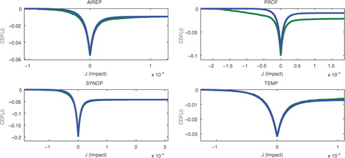
Fig. 8 Time series of the impact of the Cabauw wind profiler (PROF).

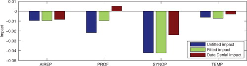
In order to verify the approximation, data denial experiments for the four assimilated observation types verified using the same observation-based metric as for the approximated impact have been conducted and are compared to the impact estimates in (Fig. 9). The order and relative magnitude of the estimated impact of surface station, aircraft and radiosondes is also reflected by their impact in data denial experiments. The impact of profilers, however, differs significantly and the data denial experiments even show a detrimental impact in contrast to the impact estimates. This is a further indication that a larger sample size would be required to assess the impact of wind profiler observations which include observations with very large impact values during a short period of convective precipitation at the Cabauw profiler site. In addition, this deviation of estimated and data denial impact is in accordance with the deviation of estimated impact and its fitted stretched exponential that is proposed as reliability indicator for the estimate.

Fig. 9 Unfitted, fitted and data denial (OSE) observation impact summed over the experimental period.

4. Conclusion

The method of Kalnay et al. (2012) provides an efficient way of assessing the value of observations in a combined LETKF-forecast system. We refined this method to use observations for forecast verification instead of the subsequent analysis to avoid the correlation of forecasts and their verification norm. In particular in presence of model biases and systematic deficiencies, the use of observations for verification is seen as advantageous approach. Based on the user interest, different weight can be given to different verifying observation types and also independent observations that are not assimilated can be used for verification. However, it needs to be kept in mind that observations are not spatially homogeneous and results are very sensitive to the applied verification norm.

We applied the refined approach in the convective-scale ensemble data assimilation system of DWD, compared results of the 6-hours forecast impact of conventional observation types using different verification norms and compared differences between estimated impact and data denial experiments in a 3-day experimental period. The largest impact per observed variable was provided by radiosonde and surface station temperature observations, followed by radiosonde wind component observations, wind profilers and aircraft observations. The largest impact per observation type was provided by surface stations as they exhibit the largest fraction of all observations.

Impact estimates verified with model analyses using a dry total energy norm showed significantly different results. A strong inter-cycle variability, however, raises concerns regarding the reliability of these estimates and a larger effect of spurious correlations using this metric.

All observation types exhibited the largest impact when the same observation type was used for verification. This is not surprising given the short forecast lead time. To some extent, this favours time-continuous observations as surface stations and profilers in contrast to temporally or spatially varying radiosondes and aircraft observations. Nevertheless, all types also showed a beneficial impact in the verification with other observations except profilers verified with surface stations and vice versa.

In a comparison with a model space based verification metric used in earlier publications, strong inconsistencies were found and associated to the correlations between forecast and the verifying analysis.

An important issue when estimating observation impact is that of the reliability of its estimate. Generally, a larger sample size and longer experimental period leads to more reliable results, but it is not yet clear how large the sample needs to be. Furthermore, the averaging requirements likely depend on the observation type and weather situation.

We found that the probability distribution of drawing a certain impact value for a single observation is an asymmetrically stretched exponential centred on the origin. By computing a fitted impact distribution function and comparing it to the unfitted one, a statement about the reliability of results can be made and a corresponding reliability indicator has been developed. This measure indicated that only the wind profilers are uncertain and probably need a larger sample size, whereas the estimates for the other observation types are reliable. In accordance, a data denial experiment for wind profiler observations showed a clear deviation from the estimated impact, whereas the results for the other observation types were overall similar for impact estimates and data denial experiments. For the experiments using the model analysis for verification, the reliability indicator also showed large values, indicating that the results are not trustworthy as derived above. This emphasises that the derived reliability indicator is a useful measure for the soundness of the estimate.

5. Acknowledgements

The authors wish to thank the data assimilation unit of DWD, specially Andreas Rhodin, Hendrik Reich and Roland Potthast for their support with the KENDA/COSMO system and helpful discussions. We are also grateful to the reviewers for their comments which helped to improve the manuscript.

The presented research was carried out in the Hans-Ertel Centre for Weather Research (Simmer, 2016; Weissmann, 2014). This German research network of universities, research institutes and DWD is funded by the BMVI (Federal Ministry of Transport and Digital Infrastructure).

References

- Baker N. L. , Daley R . Observation and background adjoint sensitivity in the adaptive observation-targeting problem. Q. J. Roy. Meteorol. Soc. 2000; 126(565): 1431–1454.
- Baker W. E. , Atlas R. , Cardinali C. , Clement A. , Emmitt G. D. , co-authors . Lidar-measured wind profiles: the missing link in the global observing system. Bull. Am. Meteorol. Soc. 2014; 95(4): 543–564.
- Baldauf M. , Seifert A. , Förstner J. , Majewski D. , Raschendorfer M. , co-authors . Operational convective-scale numerical weather prediction with the COSMO model: description and sensitivities. Mon. Weather Rev. 2011; 139(12): 3887–3905.
- Brousseau P., Desroziers G., Bouttier F., Chapnik B. A posteriori diagnostics of the impact of observations on the AROME-France convective-scale data assimilation system. Q. J. Roy. Meteorol. Soc. 2013; 140(680): 982–994. DOI: http://dx.doi.org/10.1002/qj.2179.
- Cardinali C . Monitoring the observation impact on the short-range forecast. Q. J.Roy. Meteorol. Soc. 2009; 135(638): 239–250.
- Cardinali C. , Pezzulli S. , Andersson E . Influence-matrix diagnostic of a data assimilation system. Q. J. Roy. Meteorol. Soc. 2004; 130(603): 2767–2786.
- Gasperoni N. A. , Wang X . Adaptive localization for the ensemble-based observation impact estimate using regression confidence factors. Mon. Weather Rev. 2015; 143(6): 1981–2000.
- Gelaro R. , Langland R. H. , Pellerin S. , Todling R . The THORPEX observation impact intercomparison experiment. Mon. Weather Rev. 2010; 138(11): 4009–4025.
- Gelaro R. , Zhu Y . Examination of observation impacts derived from observing system experiments (OSES) and adjoint models. Tellus A. 2009; 61(2): 179–193.
- Harnisch F. , Keil C . Initial conditions for convective-scale ensemble forecasting provided by ensemble data assimilation. Mon. Weather Rev. 2015; 143(5): 1583–1600.
- Harnisch F. , Weissmann M. , Cardinali C. , Wirth M . Experimental assimilation of dial water vapour observations in the ECMWF global model. Q. J. Roy. Meteorol. Soc. 2011; 137(659): 1532–1546.
- Hotta D . Proactive Quality Control Based on Ensemble Forecast Sensitivity to Observations. 2014; Graduate School of the University of Maryland, College Park. Doctoral thesis.
- Hunt B. R. , Kostelich E. J. , Szunyogh I . Efficient data assimilation for spatiotemporal chaos: a local ensemble transform Kalman filter. Phys. D: Nonlin. Phenom. 2007; 230(1): 112–126.
- Kalnay E., Ota Y., Miyoshi T., Liu J. A simpler formulation of forecast sensitivity to observations: application to ensemble Kalman filters. Tellus A. 2012; 64 Online at: http://www.tellusa.net/index.php/tellusa/article/view/18462.
- Kostka P. M. , Weissmann M. , Buras R. , Mayer B. , Stiller O . Observation operator for visible and near-infrared satellite reflectances. J. Atmos. Ocean. Technol. 2014; 31(6): 1216–1233.
- Kunii M. , Miyoshi T. , Kalnay E . Estimating the impact of real observations in regional numerical weather prediction using an ensemble Kalman filter. Mon. Weather Rev. 2012; 140(6): 1975–1987.
- Langland R. H . Observation impact during the north Atlantic TReC-2003. Mon. Weather Rev. 2005; 133(8): 2297–2309.
- Langland R. H. , Baker N. L . Estimation of observation impact using the NRL atmospheric variational data assimilation adjoint system. Tellus A. 2004; 56(3): 189–201.
- Langland R. H. , Rohaly G. D . Adjoint-Based Targeting of Observations for FASTEX Cyclones 9–13 September 1996. . 1996. Technical Report, DTIC Document, Seventh Mesoscale processes conference, University of Reading, UK.
- Li H. , Liu J. , Kalnay E . Correction of estimating observation impact without adjoint model in an ensemble Kalman filter. Q. J. Roy. Meteorol. Soc. 2010; 136(651): 1652–1654.
- Liu J., Kalnay E. Estimating observation impact without adjoint model in an ensemble Kalman filter. Q. J. Roy. Meteorol. Soc. 2008; 134(634): 1327–1335. DOI: http://dx.doi.org/10.1002/qj.280.
- Liu J. , Kalnay E. , Miyoshi T. , Cardinali C . Analysis sensitivity calculation in an ensemble Kalman filter. Q. J. Roy. Meteorol. Soc. 2009; 135(644): 1842–1851.
- Lorenc A. C. , Marriott R. T . Forecast sensitivity to observations in the met office global numerical weather prediction system. Q. J. Roy. Meteorol. Soc. 2013; 140(678): 209–224.
- Ota Y. , Derber J. , Kalnay E. , Miyoshi T . Ensemble-based observation impact estimates using the NCEP GFS. Tellus A. 2013; 65: 20038.
- Rabier F. , Järvinen H. , Klinker E. , Mahfouf J-F. , Simmons A . The ECMWF operational implementation of four-dimensional variational assimilation. I: experimental results with simplified physics. Q. J. Roy. Meteorol. Soc. 2000; 126(564): 1143–1170.
- Rabier F. , Klinker E. , Courtier P. H. , Hollingsworth A . Sensitivity of forecast errors to initial conditions. Q. J. Roy. Meteorol. Soc. 1996; 122(529): 121–150.
- Schomburg A., Schraff C., Potthast R. A concept for the assimilation of satellite cloud information in an Ensemble Kalman Filter: single-observation experiments. Quarterly Journal of the Royal Meteorological Society. 2015; 141(688): 893–908. DOI: http://dx.doi.org/10.1002/qj.2407.
- Schraff C. , Reich H. , Rhodin A. , Schomburg A. , Stephan K. , co-authors . Kilometre-scale ensemble data assimilation for the COSMO Model (KENDA). Q. J. Roy. Meteorol. Soc. 2016; 142(696): 1453–1472.
- Simmer C., Adrian G., Jones S., Wirth V., Göber M., co-authors. HErZ – The German Hans-Ertel Centre for weather research. Bull. Am. Meteorol. Soc. 2016. DOI: http://dx.doi.org/10.1175/BAMS-D-13-00227.1.
- Sommer M., Weissmann M. Observation impact in a convective-scale localized ensemble transform Kalman filter. Q. J. Roy. Meteorol. Soc. 2014; 140(685): 2672–2679. DOI: http://dx.doi.org/10.1002/qj.2343.
- Wahba G. , Johnson D. R. , Gao F. , Gong J . Adaptive tuning of numerical weather prediction models: randomized GCV in three-and four-dimensional data assimilation. Mon. Weather Rev. 1995; 123(11): 3358–3370.
- Weissmann M. , Folger K. , Lange H . Height correction of atmospheric motion vectors using airborne lidar observations. J. Appl. Meteorol. Climatol. 2013; 52(8): 1868–1877.
- Weissmann M. , Göber M. , Hohenegger C. , Janjic T. , Keller J. , co-authors . Initial phase of the Hans-Ertel Centre for weather research – a virtual centre at the interface of basic and applied weather and climate research. Meteorol. Z. 2014; 23(3): 193–208.
- Weissmann M. , Harnisch F. , Wu C.-C. , Lin P.-H. , Ohta Y. , co-authors . The influence of assimilating dropsonde data on typhoon track and midlatitude forecasts. Mon. Weather Rev. 2011; 139(3): 908–920.
- Weissmann M. , Langland R. H. , Cardinali C. , Pauley P. M. , Rahm S . Influence of airborne doppler wind lidar profiles near typhoon Sinlaku on ECMWF and NOGAPS forecasts. Q. J. Roy. Meteorol. Soc. 2012; 138(662): 118–130.