A systematic method of parameterisation estimation using data assimilation

Abstract

In numerical weather prediction, parameterisations are used to simulate missing physics in the model. These can be due to a lack of scientific understanding or a lack of computing power available to address all the known physical processes. Parameterisations are sources of large uncertainty in a model as parameter values used in these parameterisations cannot be measured directly and hence are often not well known; and the parameterisations themselves are also approximations of the processes present in the true atmosphere. Whilst there are many efficient and effective methods for combined state/parameter estimation in data assimilation (DA), such as state augmentation, these are not effective at estimating the structure of parameterisations. A new method of parameterisation estimation is proposed that uses sequential DA methods to estimate errors in the numerical models at each space-time point for each model equation. These errors are then fitted to pre-determined functional forms of missing physics or parameterisations that are based upon prior information. We applied the method to a one-dimensional advection model with additive model error, and it is shown that the method can accurately estimate parameterisations, with consistent error estimates. Furthermore, it is shown how the method depends on the quality of the DA results. The results indicate that this new method is a powerful tool in systematic model improvement.

• data assimilation
• parameterisation estimation
• parameter estimation

1. Introduction

Data assimilation (DA) is the process by which observational data are incorporated into numerical models to improve knowledge of the trajectory, and uncertainties, of the state. In meteorological models, DA is used to generate an optimal initial state to be used in subsequent forecasts through the use of prior knowledge of the state (e.g. a previous forecast) and observational data obtained from satellites/weather stations, etc. This combination of prior information and observational data is commonly referred to as state estimation.

Models have parameters that are often unobservable quantities, such as latent heat flux, entrainment rate and surface albedo. Using observations to infer the values that these parameters take is known as parameter estimation. Parameter estimation is a more complex problem than state estimation, as even for simple, linear models, the parameter estimation problem becomes non-linear (Evensen et al., 1998). The majority of parameter estimation methods are based on some form of state augmentation, where the state vector is augmented, or extended, with a vector of parameter values. This allows the parameters to be estimated via the DA analysis equations in the same manner that any unobserved prognostic variables would be updated. In a sequential DA scheme, this would involve updating the parameters at every observation time during the model run.

State augmentation is an effective method of parameter estimation and is used to estimate optimal parameters with varying degrees of success (e.g. Annan et al., 2005; Kondrashov et al., 2008; Smith, 2010). However, the process of changing the parameters during a model run may lead to parameters being modified to a region of dynamical instability which may cause the model run/state estimation to fail (Yang and Delsole, 2009; Williamson et al., 2014). Another common problem with state augmentation is that the parameter ensemble tends to collapse before an optimal parameter value is found (Santitissadeekorn and Jones, 2014). This can be mitigated by adding a small perturbation to the parameter in order to stop the ensemble from collapsing before the optimal parameter is found. However, the method of generating the perturbation to add to the parameter value is not well understood, with suggestions for improving the parameter ensemble in Liu and West (2001). State augmentation methods, however, cannot be used to estimate systematic functional errors in the parameterisations.

Parameterisations are functions that represent simplified forms of processes in the models that are either sub-grid scale processes or are too complex (either due to lack of scientific understanding or not enough computational power) to represent explicitly. For example, in numerical weather prediction (NWP) models, parameterisations are used to approximate processes such as convective processes, cloud microphysics and radiative processes.

Parameterisation estimation is even more complex than parameter estimation, as it requires not only the estimate of correct parameters, but also the estimate of the functional form of the parameterisation itself. Furthermore, as parameters/parameterisations do not necessarily represent true physical qualities that occur within a system, rarely are they observed quantities.

Parameterisation estimation is often done in an ad-hoc way by running models using the current parameterisations and compensating for errors in the functional forms by adding new parameters or functions when they arise. However, these new additions may not improve a fundamental error with the parameterisation. This is because forecasts are often verified against reanalysis data every 1–6 hours, hence errors have time to accumulate making it difficult to infer the source of the errors.

In this study, DA is used to obtain information about errors in the numerical models, specifically errors that come from incorrectly specified parameterisations. A new method of parameterisation estimation is proposed that makes use of the model equations that will allow for an estimate of the structure in the model errors to be found. This new method uses the differences between a DA analysis and an analysis forecast to estimate the errors in the parameterisations each space-time point. In this study, this parameterisation estimation method is applied to an advection model with additive model error as it is a simple model where it is well known how changes in the functional form affect the dynamics of the system.

This paper shall describe the DA methods used in Section 2. Section 3 outlines the new parameterisation estimation method that is proposed by this study, followed by numerical results and conclusions in Sections 4 and 5, respectively.

2. Data assimilation methods

In this section, the data assimilation method used in this study, the ensemble Kalman smoother (EnKS), is described, and the notation used throughout this paper is introduced.

2.1. Ensemble Kalman Filter

The ensemble Kalman filter (EnKF) was developed by Evensen (1994) and has many different variations that are mainly split into two groups. There are the stochastic EnKFs, such as developed by Burgers et al. (1998) and Houtekamer and Mitchell (1998); and the Ensemble Square Root Filters [EnSRF, Tippett et al. (2003)], including the ensemble adjustment Kalman filter [EAKF, Anderson (2001)] and the ensemble transform Kalman filter [ETKF, Bishop et al. (2001) and Majumdar et al. (2002)]. This study shall use the stochastic EnKF [from Burgers et al. (1998)] but any of the other methods can be used.

The EnKF is a sequential DA method that uses Monte Carlo methods to approximate the error statistics of the state. The evolution of the state is given by the following equation:1 where x(t) is the N-dimensional state vector at time t, represents the deterministic model and ξ is an unknown model error (assumed to be random).

The EnKF approximates the forecast error covariance matrix, , by using an ensemble of M distinct state vectors at time t, X(t), such that:2 where represents an N-dimensional ensemble member of the forecast state and is the mean over the ensemble.

The k ^th set of observations (occurring at timestep t _k ) denoted y _k with an observation error ε _k is assumed to be Gaussian, with zero mean and a covariance matrix given by (where p _k is the dimension of y _k ). The observations are related to the state by:3 where is the k ^th observation operator that maps the state vector to observation space and x ^t is the true state.

The initial ensemble is created by sampling ensemble members from a (normal) distribution centred on the initial background state with covariance matrix, , generated from prior information. The ensemble is then propagated forward using the model equations to the observation time, at which point the state is updated by the formula:4 where is the m ^th ensemble member of the updated analysis at timestep t _k , δ _m is a stochastic perturbation added to the observation operator that has the same distribution as ε _k and K _k is the Kalman gain matrix for the k ^th observation with the form5 where H _k is the linearisation of .

The result is a new analysis ensemble of state vectors which are then propagated forward by the model. The process is repeated every time there is an observation.

When using the ensemble to estimate the forecast error covariance matrix, spurious correlations can arise in the ensemble covariance matrix that would not occur in the full forecast error covariance matrix. The method used to reduce the impact of these spurious correlations is localisation [see, for example Houtekamer and Mitchell (2001) and Janjic et al. (2011)]. To do this, a localisation function, is defined, typically a function of distance in the spatial domain. The localisation matrix, is defined, where i and j are points in the domain and is applied to via the Schur, or Hadamard, product such that:6 where is the localised forecast error covariance matrix and ○ represents the Schur product of the two matrices.

2.2. Ensemble Kalman Smoother

The EnKS was developed by Evensen and van Leeuwen (2000) and is an extension of the EnKF that aims to update the state vector between observations. This is done by considering the temporal cross-covariances between the model state at the analysis timestep and the observation timestep to update the state accordingly. The first step of the EnKS is to run the EnKF to the observation time, t _k , to obtain the analysed state vector, . The ensemble forecast cross-covariance matrices between timesteps t _l and t _k are then calculated as:7 where .

The m ^th ensemble member of the state vector at t _l is then updated using the following equation:8 where the Kalman gain matrix, K _kl , between t _k and t _l is defined as:9 The difference between the EnKS and the EnKF is now the observations influence the trajectory between observation timesteps as opposed to only at the observation timestep.

3. The parameterisation estimation method

In this section, we discuss a new algorithm for parameterisation estimation using a DA scheme. Traditionally, new parameterisations are chosen by making a large number of forecasts with different parameterisation versions in the model and testing which verifies the best. The method that we propose identifies errors in the functional form of the model (i.e. the model equations) based upon results obtained from a sequence of DA steps. The methodology is general and will apply to any numerical model of any dimension. Let the true state vector at timestep t be denoted by x(t). Hence, the evolution of this state over one timestep can be written as:10 where f is the deterministic part of the model, G is the parameterisation we wish to estimate with input parameters given by α, and ξ(t) is a stochastic forcing term representing model error.

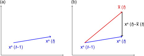
Fig. 1 A single timestep from the data assimilation trajectory from timestep t−1 to t. Step 3 defines as a single model timestep from the data assimilation trajectory at timestep t−1 using the model f with the prior parameterisation G ^b .

The method consists of two parts: (1) finding an estimate of the model error at every space-time point and every variable and (2) extract the structural part of the model error and generate a new parameterisation.

Part I: Estimation of model errors via state estimation

1. Given forecast state , background parameterisation G ^b , with background parameters α ^b , and y, perform state estimation to produce an analysis trajectory, x ^a(t) for all timesteps.

2. Define an analysis forecast variable, by running the model forward one timestep using the prior parameterisation, such that , for all timesteps. Note that each starting point is from the analysis trajectory, in Fig. 1b.

3. Compute over the whole spatial domain at every timestep. This is the difference between a model forecast of one timestep and the analysis, and contains information about structural errors in the model equations.

   Part II: Estimation of parameterisation errors that give rise to model error

4. Using any available prior information, propose a collection of n potentially missing parameterisation terms which may contribute to the parameterisation error.

5. Group these terms into sets of test functions, g _i , that contain the first i+1 terms, such that .

6. Use an optimisation scheme to fit the differences between the analysis and analysis forecast, e(t), to all of the functions, g _i .

7. Use Bayesian Information Criterion (BIC) to find the terms that contain the most information about the model error.

8. Reorder the terms in ascending order of BIC differences and define a new set of functions, h _i , such that each contain the first i+1 reordered terms.

9. Repeat Steps 5 to 7 for the new test functions, h _i , to determine the dominant terms that are missing from the model.

10. The function corresponding to the minimum BIC value corresponds to the optimal functional form of the model error, h ^* given the test function, g.

11. The new estimate for the true state is G ^a =G ^b +h ^* .

12. Fit the e (t) for each ensemble member using the terms in the optimal functional form and h ^* as a first guess to obtain an ensemble of functional forms for the true model error. The error variance for each functional form from the fit is averaged over the ensemble members to obtain a final error estimate of the parameterisation.

3.1. Explanation of algorithm

The most important ingredient of this new method is that concentrates on estimating parameterisations at the level of the model equations directly, and not after errors have accumulated after several timesteps. In the latter case, it will be very difficult to unravel the cause of the accumulated model error in non-linear models.

The first step of the parameterisation estimation method is to run a DA scheme with a prior estimate of the parameterisation, G ^b , generating a time series of analysis state vectors, x ^a (t) which represent the best estimate of the true state through time.

Using the time series of x ^a (t) values generated, a new time series representing a forecast of the analysis state, , is generated such that:11 The difference between the analysis and the analysis forecast at all analysis timesteps for each variable at each grid-point is given by , illustrated for a single timestep in Fig. 1, which represents the best estimate that is currently available regarding the model error at each timestep in each model equation. In order to extract the functional form of this term, a test function needs to be defined to compare the structure in .

The terms chosen in Step 3 can be arranged into a function of the form:12 where are the coefficients to be computed in an optimisation scheme. The are functions of the state variable that may include derivatives of the state. ξ represents the stochastic model error assumed to be Gaussian with zero mean and covariance determined by the fit. It is important that the terms are specified well, as this parameterisation estimation method will only look for possible parameterisations in the span of the function . Without any prior information, finding a true parameterisation is an ill-posed problem. The prior information and therefore the terms to be considered are generally obtained with help from an expert with knowledge of likely errors in the model. These may include terms assumed negligible such as higher order terms.

Using this form, the parameterisation estimation problem has been translated into a parameter estimation problem, also known as regression analysis. By using an optimisation scheme to calculate the optimum coefficients, , for the test function, a functional estimate for the errors in the parameterisation will be found. The choice of optimisation scheme is free; for simplicity, we have chosen linear regression, but non-linear regression or sparse regression techniques, etc. may be used.

This is done sequentially by using the optimisation scheme to initially estimate the coefficient for the first term in g, . In other words, the first test function is defined as:13 and β ₀ is calculated by using the optimisation scheme to fit to .

The test function is then updated to include the first and second terms of and the optimisation scheme is used again to fit to:14

This is repeated until functional estimates are obtained for all g _i , .

To verify the quality of the functional estimates calculated in the above step, the BIC (Schwarz, 1978) is used. The Akaike Information Criterion AIC, Akaike (1974) can also be used and produces similar analysis. The BIC is given by:15 where k is the number of parameters used in the test function, N is the number of points in and is the maximised likelihood function, . The BIC represents the trade-off between how well the functional estimate fits against the complexity of the model. The BIC is a quantification of Occam's razor states that the optimal form of the parameterisation is the simplest form of the parameterisation that fits the data well. As the regression produces a better fit to , the log-likelihood term () increases, resulting in a decrease in BIC. However, as the number of terms in the functional estimate increases, the BIC increases, hence punishing overly complex models. This implies that the optimal form of the parameterisation is given when the BIC is minimal.

When the BIC has been calculated for all g _i functions in Step 6, the terms whose addition to the test function coincide with the biggest decreases in BIC from g _i–1 to g _i (where the decrease from g ₋₁ to g ₀ is defined as 0) will contain the most information about the structure of .

In Step 8, the terms in g are then reordered in descending order of terms with the greatest decrease in BIC to create a new functional form for the model error, h(x). h(x) is then split into sub-functions in the same way as g(x) and the optimisation scheme is again run for each h _i (x) and the coefficients are calculated as before. As the terms are now ordered such that the terms with most information in them are first in the test functions, the BIC will decrease until it reaches the optimal function and then increase for all functional forms after that. Therefore, the minimum in the BIC calculated for each h _i (x) will correspond to the optimal functional form of the model error, within the set that is being considered.

By calculating the coefficients for all h _i (x) individually, we obtain a set of functions with various degrees of confidence based upon the BIC (i.e. the lower the BIC is for an estimate, the higher the confidence in that functional estimate).

To calculate the uncertainty in the coefficients obtained from the method, the uncertainties in the coefficients obtained from each ensemble member are averaged over the ensemble.

For example, for least-squares (used in the results in this paper), the error covariance matrix for the parameters is obtained as (Friedman et al., 2001):16 where is a matrix of all the functions, f _i , in the test function at all N gridpoints and all T timesteps and is the variance of the resulting random errors from the regression, such that:17 where is the function obtained from the least squares fit of the over all space-time points.

4. Numerical experiments

In this section, experiments are performed on an imperfect 1D advection model described by the following continuous equation:18 where s is the space dimension, t is time, α is the linear component of the advection velocity and is a stochastic term representing the model error present in the system. x(t) is the quantity being advected, and is a scalar at each point in space-time. In the notation outlined in the previous section, x(t) is the collection of x at all gridpoints at timestep, t. G is an additive parameterisation of the – possibly non-linear – model error present in the advection equation and is the parameterisation that we shall estimate in the following experiments.

The advection model is applied to a sine wave advected for 100 timesteps over a periodic domain on the interval [0,1] with 101 gridpoints spread uniformly across it, such that Δs = 0.01.

The initial true state is defined as:19 where the initial model errors are distributed normally with covariance given by a Second Order Autoregressive (SOAR) function, that is:20 where k and l are two gridpoints, d(k,l) is the shortest distance between k and l, and L = 0.06 is a correlation length scale.

For subsequent timesteps, the model error, is distributed by an uncorrelated Gaussian distribution with zero mean and error covariance, .

The initial state covariance of the ensemble is also given by a SOAR function, but with a smaller correlation length scale of 0.05. SOAR functions are used in order to introduce cross-covariances between gridpoints.

Observations at timestep, k, are taken of the true state directly such that:21 where observation errors, , are distributed normally with zero mean and error covariance, R _k , where (p _k is the number of observations at timestep k). It is assumed that each observation is independent, hence R _K is diagonal. Unless otherwise stated, observations are taken at all timesteps and gridpoints in the following experiments.

The EnKS is used with 40 ensemble members and localisation applied to the P ^f matrix in the space dimension, using the localisation function:22 where the localisation radius, R _loc , is defined as 0.1 for these experiments.

The initial test function for use in the parameterisation method is defined as:23 The terms were chosen as they may appear in an advection model, and each has a physical meaning. The x terms represent the quantity being advected, is the velocity of the advection and represents diffusion.

The optimal functional difference, as calculated by our parameterisation estimation method for each experiment is presented with uncertainty specified on each coefficient calculated as the standard deviation of the parameter errors averaged over the ensemble, as described in Section 3.1.

4.1. Linear advection model

In this section, the method outlined in Section 3 will be applied to a simple parameter estimation problem where the only structural/deterministic error in the model comes from an error in a scalar parameter.

A true state trajectory, x ^t is generated using:24 and a true parameterisation value of the form:25 which we wish to estimate.

The background state/initial estimate of the true state trajectory, x ^b is generated using the parameterisation of the form:26 Substituting these values into the true and background models given in eq. (18) leads to a true model given by:27 and a background model28 Each model described in eqs. (27) and (28) is integrated using a upwind Euler scheme with timestep:29 in order to maintain the Courant–Friedrichs–Lewy (CFL) criterion. This value of Δt is chosen to minimise spurious numerical diffusion in the experiments.

Using the method outlined in Section 3, the optimal functional form of the parameterisation, G, is given by:30 This is very close to desired solution given in eq. (25). The true parameterisation falls within the error, generated from the ensemble, of the function obtained by this method.

In addition to the simple adjustment of parameter, it can be seen that the parameterisation estimation method also calculates the numerical diffusion that occurs in the system. Analytical calculations show that the expected difference in numerical diffusion produced by the upwind scheme between the true and background models (with no model error) is , which is within the uncertainty estimated by the parameterisation estimation method.

4.2. A non-linear advection equation

In this experiment, the true state is no longer generated by the linear advection equation, instead it is generated with:31 and truth parameterisation:32 This leads to a true model given by:33 The introduction of the state variable into the advection equation leads to the model becoming non-linear. The non-linear term, , has the effect of steepening the gradient of the sine wave between the peak and trough of the sine wave, by making the peak move faster and the trough slower.

The background model shall continue to assume that the truth is generated by a linear advection model such that the background parameterisation is given by:34 Therefore, the background model becomes:35 The advection speed, α = 4.5, is chosen such that the background advection velocity is approximate to the advection velocity of the peak of the non-linear advection model in equation.

The initial conditions are the same as the previous experiments on the linear advection model in Section 4.1. The value of Δt is changed to fulfil the CFL criterion of the non-linear advection model and is now given by36 where 22.5 is chosen such that the system is comfortably within the stable regime of the upwind Euler scheme.

The parameterisation estimation procedure gives an estimate of the true parameterisation in the form37 Comparing this to eq. (33) indicates that this is a consistent estimate of the true parameterisation given the estimated errors.

4.2.1. State augmentation.

In this section, the new method of parameterisation estimation is compared with an existing method of parameter estimation, state augmentation, when applied to the estimation of parameterisations. The true and background models and observation density are the same as in Section 4.2. It is unknown how to define a localisation matrix such that the augmented forecast error covariance matrix is positive definite. This is due to the bordering entries in the augmented localisation matrix, corresponding to the cross-covariances between the state and parameters; setting these to be one can destroy the definiteness of the matrix. This results in non-positive eigenvalues occurring in the ‘localised’ augmented forecast covariance matrix. Therefore, a 2000-member ensemble is used in the EnKF such that localisation is not required to account for spurious correlations in the forecast covariance matrix.To extend state augmentation to the estimation of parameterisations, we again assume that the true model error terms are unknown and add the full test function defined in (23) to the background model. So that the augmented background model for state augmentation becomes:38 The a _i 's are the parameters to be estimated using state augmentation, and the results obtained are summarised in Fig. 2. The parameterisation error found through using state augmentation is:39 Therefore, the analysis model obtained from state augmentation is:40 It can be seen that this form of the parameterisation error does not recreate the true model error , from eq. (32). This is not the simplest parameterisation error possible, and no information is obtained from state augmentation that suggests how important the terms are relative to one another so that the number of terms in the test function can be reduced.

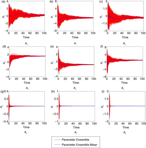
Fig. 2 Estimated parameter values from state augmentation, for the parameters described in eq. (38).

4.3. Experiments with different observation densities

The aim of this section is to show the sensitivity the parameterisation estimation method to the quality of the state estimation. This is done by reducing the observation density in space and/or time resulting in a less accurate DA trajectory.

The experiments in this section, shown in Table 1, will have the same true and background parameterisations as in Section 4.2, such that the true state is generated from the non-linear advection eq. (33) and the background state is generated from the linear advection eq. (18). The observation error covariance matrix and stochastic model error covariance matrix and the localisation function and radius are the same as used in Section 4.1.

Table 1. Analysis parameterisations from parameterisation estimation method for different observation densities

Observations at all space-time points
Observations at every three gridpoints and every timestep
Observations at every gridpoint and every three timesteps
Observations at every three gridpoints and every three timesteps

It can be seen in Table 1 that when the observation density decreases, the parameterisation estimation method produces less accurate estimations of the true parameter values. This is due to the observations not being able to fully constrain the DA analysis to the true state. When observations are taken every three gridpoints, the diffusion terms become more prominent. However, they are always within the error bounds specified by our methods. When observations are taken every gridpoint and every three timesteps, the parameterisation estimate falls outside the one-standard deviation error bound from the truth, but only slightly. In all other cases the estimates are consistent.

4.4. Relation between magnitudes of stochastic model error and stochastic observation error

In this section, we study the sensitivity of the method by varying the relative magnitude of model error covariance matrix, Q, and observation error covariance matrix, R.

The true model and background models are both generated using eqs. (33) and (18), from Section 4.2, respectively and to ensure that the CFL criterion is conserved. The experiments are performed in the well-observed case where observations occur at all space-time points and the same localisation function is used as in Section 4.1, given by eq. (22) with localisation radius, .

Recall that in the previous experiments, Q=0.01² I and R=0.05² I (i.e. Q=4R) and that the experiments in this section should be compared directly with the experiment in Section 4.2.

Table 2 shows that the parameterisation terms become less accurate when R increases compared to Q, but estimated errors also increase in a consistent manner. Additionally, the diffusive terms become more prominent as R increases.

Table 2. Analysis parameterisations from parameterisation estimation method for different magnitudes of observation error relative to model error

R=0.005^2 I such that Q=4R
R=0.01^2 I such that Q=R
R=0.02^2 I such that Q = 0.25R

This is because as the observation error covariances increase relative to the model error covariances, the state estimation will have more confidence in the prior model with respect to the observations meaning that the analysis state will be closer to the prior model equations, hence the signal in the observations will be much weaker. As a result, the diffusion terms become more prominent in the analysis state. This is to be expected, as the observations do not contain enough information to get the functional estimate closer to the desired solution.

5. Conclusions

This study has presented a new method of parameterisation estimation that uses the model equations directly to estimate the underlying errors in the model. This is done by comparing the DA analysis with an analysis forecast at every space-time point for every model variable to retrieve errors in the model and to use this information to improve model parameterisations. It is important to realise that the method uses the errors at the level of the model equations directly, instead of accumulating errors over a number of model timesteps. In the latter case, it is difficult to find the cause of the errors in a non-linear model, as model equation errors will interfere with each other during the accumulation. As the method uses the DA analysis as the best estimate of the truth, this method is dependent on the quality of the DA analysis.

In this paper, experiments have been shown using the linear advection equation to estimate parameters. Existing methods of parameter estimation are mostly based on state augmentation, which is an online method where the parameters are updated along with the state. While this means that state augmentation is potentially more computationally efficient, there is a risk that the updated parameter values could cause the numerical model to become unstable (e.g. for the advection models, an advection velocity could be updated such that the CFL criterion is violated) in the middle of computation. For simple parameter estimation, state augmentation may give a better estimate of the true parameter values. However, our new method has been developed to find overall structural errors in the model where state augmentation cannot. There is no risk of numerical instability with our method, as it is an offline method. Model runs are only computed with background parameterisations.

In the numerical experiments conducted in this paper, when the DA analysis was poor, due to less accurate observations or due to a less dense observations network, poorer estimates of the model error were obtained. This meant that was less representative of the true model error present in the system, hence the optimal equations obtained from the regression were less representative of the true model error. It is worth noting that the diffusion terms become more prominent when there are fewer observations in space, and that our method is also able to estimate the scale of numerical diffusion present in system. Our method does provide an error estimate on the new parameterisation which is related to the spread in the ensemble. So a less accurate DA result will lead to a larger error in the parameterisation estimate, leading to consistent estimates even if the DA is poor.

The method introduced in this study will only find parameterisations within the pre-determined functional form. Our method appeals to the BIC to select the most influential terms. The optimal equation for the true model error corresponds to the equation with the lowest value of the BIC.

Work still needs to be done to reduce the sensitivity of the method to the quality of the analysis state in order to produce better/more consistent estimates of the model error. However, the new method of parameterisation estimation presented in this study has been shown to estimate simple parameterisations and has the potential to estimate functional forms of model errors and hence parameterisations in more complex models. A natural application of this method would be to infer parameterisations for a low-resolution model when a higher resolution model is available. In this case, all variables can be observed which is favourable for this method. We are currently planning to test the method on NWP models.

6. Acknowledgements

This work is funded by the Natural Environment Research Council under NE/J005878/1 and via the National Centre for Earth Observation (PJvL).

References

- Akaike H . A new look at the statistical model identification. IEEE Trans. Automat. Contr. 1974; 19(6): 716–723.
- Anderson J. L . An ensemble adjustment Kalman filter for data assimilation. Mon. Wea. Rev. 2001; 129(12): 2884–2903.
- Annan J. D. , Hargreaves J. C. , Edwards N. R. , Marsh R . Parameter estimation in an intermediate complexity earth system model using an ensemble Kalman filter. Ocean Model. 2005; 8(12): 135–154.
- Bishop C. H. , Etherton B. J. , Majumdar S. J . Adaptive sampling with the ensemble transform Kalman filter. Part I: Theoretical aspects. Mon. Wea. Rev. 2001; 129(3): 420–436.
- Burgers G. , van Leeuwen P. J. , Evensen G . Analysis scheme in the ensemble Kalman filter. Mon. Wea. Rev. 1998; 126(6): 1719–1724.
- Evensen G . Sequential data assimilation with a nonlinear Quasi-Geostrophic model using Monte-Carlo methods to forecast error statistics. J. Geophys. Res. Oceans. 1994; 99(C5): 10143–10162.
- Evensen G. , Dee D. P. , Schröter J . Chassignet E. P. , Verron J . Parameter estimation in dynamical models. Ocean Modeling and Parameterization. 1998; Springer, Netherlands. 373–398.
- Evensen G. , van Leeuwen P. J . An ensemble Kalman smoother for nonlinear dynamics. Mon. Wea. Rev. 2000; 128(6): 1852–1867.
- Friedman J. , Hastie T. , Tibshirani R . The Elements of Statistical Learning. 2001. 2nd ed. Springer, Berlin.
- Houtekamer P. L. , Mitchell H. L . Data assimilation using an ensemble Kalman filter technique. Mon. Wea. Rev. 1998; 126(3): 796–811.
- Houtekamer P. L. , Mitchell H. L . A sequential ensemble Kalman filter for atmospheric data assimilation. Mon. Wea. Rev. 2001; 129(1): 123–137.
- Janjic T. , Nerger L. , Albertella A. , Schröter J. , Skachko S . On domain localization in ensemble-based Kalman filter algorithms. Mon. Wea. Rev. 2011; 139(7): 2046–2060.
- Kondrashov D. , Sun C. , Ghil M . Data assimilation for a coupled ocean-atmosphere model. Part II: Parameter estimation. Mon. Wea. Rev. 2008; 136(12): 5062–5076.
- Liu J. , West M . Doucet A. , de Freitas N. , Gordon N . Combined parameter and state estimation in simulation-based filtering. Sequential Monte Carlo Methods in Practice. 2001; 197–223. Statistics for Engineering and Information Science. Springer, New York.
- Majumdar S. J. , Bishop C. H. , Etherton B. J. , Toth Z . Adaptive sampling with the ensemble transform Kalman filter. Part II: Field program implementation. Mon. Wea. Rev. 2002; 130(5): 1356–1369.
- Santitissadeekorn N. , Jones C . Two-state filtering for joint state-parameter estimation. arXiv preprint arXiv:1403.5989. 2014
- Schwarz G . Estimating the dimension of a model. Ann. Stat. 1978; 6(2): 461–464.
- Smith P . Joint state and Parameter Estimation using Data Assimilation with Application to Morphodynamic Modelling. 2010; University of Reading, UK: PhD Thesis.
- Tippett M. K. , Anderson J. L. , Bishop C. H. , Hamill T. M. , Whitaker J. S . Ensemble square root filters. Mon. Wea. Rev. 2003; 131(7): 1485–1490.
- Williamson D. , Blaker A. T. , Hampton C. , Salter J . Identifying and removing structural biases in climate models with history matching. Clim. Dyn. 2014; 45(5–6): 1299–1324.
- Yang X. , Delsole T . Using the ensemble Kalman filter to estimate multiplicative model parameters. Tellus A. 2009; 61(5): 601–609.