Examination of Hurricane Sandy's (2012) structure and intensity evolution from full-field and anomaly-field analyses

Abstract

An anomaly-based field analysis approach and a set of simple beta-advection models (BAMs) have been used to examine the structure evolution and unusual left turn of Hurricane Sandy (2012) before it made the landfall and caused severe damage along the eastern US coast. Results show that the anomaly-based analysis approach can clearly reveal Sandy's structure evolution, including its interaction with other synoptic-scale systems as well as the intensification and extratropical transition (ET) processes. During its lifetime, Sandy experienced two consecutive periods of intensification caused by the merging of anomalous vortices on 27 and 29 October. The unusual left turn and the ET process prior to the landfall are respectively influenced by an anomalous anticyclone to the northeast and an anomalous cold vortex at the 300–850 hPa layer to the northwest, which is confirmed by the experiments using the generalised BAM.

• Hurricane Sandy
• anomaly
• intensification
• extratropical transition
• model forecast

1. Introduction

Previous studies have shown that tropical cyclone (TC) motions are mainly governed by the tropospheric average steering flow (Chan and Gray, 1982). During summer and autumn, TCs in the Northwest (NW) Atlantic and NW Pacific generally move westward, northwestward, or northward. The TCs are mainly driven by large-scale steering flow associated with the dominant subtropical high and the transient synoptic waves from the west in middle and high latitudes. The possibility for a TC to recurve into the westerly flow depends on the strength of the subtropical high. If encountering a weakening process in the subtropical high ridge, a TC often propagates northeastward as it moves into the westerly flow, which is considered as the normal track (George and Gray, 1976). However, the classic recurving track exhibits a great variability because both the strength of the subtropical high and the amplitude of the mid- and high-latitude wave trains contribute to the left or right turnings. The unusual TC turnings occur despite a typical steering flow and the reasons for the turnings are not obvious from the inspection of the traditional synoptic charts. Recently, Huang et al. (2015) and Qian et al. (2015) respectively applied an approach of decomposing a full or total atmospheric variable into a climatic component and an anomaly to study the unusual left-turning motion of four TCs in the East China Sea (ECS) and the intensity evolution of super Typhoon Megi (2010) in the South China Sea (SCS). Their results showed that the anomaly-based analysis and a set of simple beta-advection models (BAMs) can explain the unusual tracks of TCs in the ECS and SCS (Qian et al., 2014, 2015; Huang et al., 2015). The generalised beta-advection model (GBAM) is one of the simple BAMs, which is able to predict the location of an anomalous vorticity centre. It is run at an optimal pressure level of the maximum anomalous vorticity centre. All unusual right-turning tracks of TCs in the SCS and left-turning tracks of TCs in the ECS during the last 30 yr can be well predicted by the GBAM with 2–3 d in advance, but they cannot be correctly predicted by the climatic-flow beta-advection model (CBAM) or the anomaly-flow beta-advection model (ABAM) nor classical BAMs (Qian et al., 2014; Huang et al., 2015). The reason is that the GBAM takes the combined effect from the climatic steering flow and the interaction with anomalous systems into account.

Over the Atlantic, the infamous Hurricane Sandy (2012) was an unusual left-turning TC and its rapid intensification caused tremendous damage along the Mid-Atlantic and New England regions upon its landfall shortly before 0000 UTC 30 October 2012. In coastal area, the worst damage was caused by the storm surge, leading to floods in New York City and its surrounding areas (Galarneau et al., 2013; Chen et al., 2014). Sandy caused local floods and sustained hurricane-forced wind along the coast while the high elevation areas in the Appalachians experienced cold and heavy snowfall (Magnusson et al., 2014). Advanced warning of TCs such as Sandy is essential for saving lives and protecting properties (Malakoff et al., 2012; Burger and Gochfeld, 2014). The global model of the European Centre for Medium-Range Weather Forecasting (ECMWF) provided an excellent forecast of Sandy's landfall location up to 1 week in advance (Bassill, 2014; Knabb, 2013; Uccellini, 2013). Despite this success, it is of scientific interest to understand the underlying dynamical processes that are responsible for the rapid left turn and intensification of Hurricane Sandy prior to its landfall. Using a stochastic model, Hall and Sobe (2013) estimated that the return period for an event like Hurricane Sandy was over 700 yr in terms of its intensity and landfall. Their finding implies that Sandy is an abnormal event in the stages of intensification and landfall. Unlike the conventional synoptic analysis, the anomaly-based analysis may be useful for the study of Sandy (2012) in the Atlantic.

In this paper, we first demonstrate the advantages of the anomaly-based analysis over the traditional full-field-based analysis to reveal the evolution of Sandy's structure including its interaction with other systems, intensification and the final extratropical transition (ET) process using reanalysis data. Then, the unusual left turn of Sandy influenced by other systems is dynamically explored using different BAMs. This paper is organised as follows. Section 2 describes the Sandy case and data sets. Section 3 describes (1) the methodology used for extracting anomalous information and (2) different BAMs used in this study. Results are presented in Section 4 and conclusions are in Section 5.

2. Sandy case and data sets

2.1. Sandy case

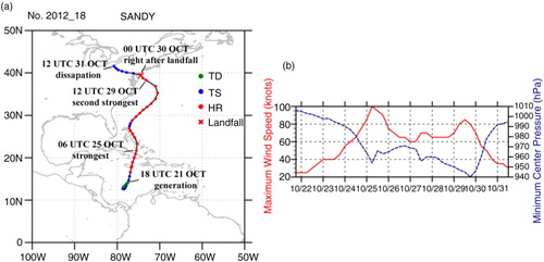
We first describe the evolution of Hurricane Sandy (2012). The ‘best track’ of the cyclone's path, starting at 1800 UTC 21 October 2012, is given in Fig. 1a with the maximum wind speed and pressure evolution shown in Fig. 1b. Surface and satellite data suggested that a low pressure circulation became well defined about 200 NM south of Jamaica on 21 October 2012 (www.nhc.noaa.gov/data/tcr/AL182012_Sandy.pdf). At the very first stage, Sandy first moved southwestward slowly for about 1 d as a tropical depression (TD) and then returned northward for about 2 d as a tropical storm (TS). It intensified into a hurricane (HR) quickly by late 23 October and continually moved northward. Its strongest intensity (the first peak wind speed) was estimated at 0600 UTC 25 October. Six hours later, it turned northwestward for about 1 d. It weakened into a TS at 0000 UTC 27 October for a half day and turned northeastward entering the NW Atlantic. Starting at 1200 UTC 27 October, Sandy intensified again into a HR (the second peak wind speed). After 0000 UTC 29 October, it turned left suddenly to the northwest and reached its third peak wind speed of 85 kt around 1200 UTC and the lowest central pressure of 940 hPa at around 1800 UTC 29 October. Five and a half hours later (around 2330 UTC 29 October), it made landfall near Brigantine, New Jersey, just north of Atlantic City as a ‘post-tropical’ cyclone. After landfall, it moved westward inland and dissipated at 1200 UTC 31 October 2012.

Fig. 1 (a) Best track and (b) intensity evolution indicated by maximum wind speed (red solid line, knots) and minimum central pressure (blue dashed line, hPa) of Hurricane Sandy with 6-hour interval from 1800 UTC 21 October to 1200 UTC 31 October 2012. It formed at 1800 UTC 21 October with the strongest wind speed at 0600 UTC 25 October, the second peak at 1200 UTC 27 October and the third peak at 1200 UTC 29 October, landfall near 0000 UTC 30 October, and dissipation at 1200 UTC 31 October 2012. Sandy was classified as tropical depression (TD), tropical storm (TS) and hurricane (HR) during its lifetime.

2.2. Data sets

Two data sets are used in this study. The ECMWF Re-Analysis Interim (ERA-Interim) provides a set of four-dimensional variational (4D-Var) reanalysis. It has a 0.75°×0.75° latitude-longitude resolution ranging from 1979 to current (satellite era started in 1979). The climatology of three basic variables, geopotential height, temperature and wind at standard pressure levels from 1000 to 50 hPa, is derived from a 30-yr period (1981–2010) of this data. The second data set is the revised Atlantic hurricane database HURDAT2 provided by the National Hurricane Center (NCEP/NHC), which is based on the traditionally disseminated TC historical database in the format known as HURDAT (Jarvinen et al., 1984). It provides the best track of Hurricane Sandy.

3. Approach and models

3.1. Approach

An atmospheric total or full field such as geopotential height, temperature and zonal (meridional) wind (u and v) at diurnal time t (24 hours a day), for a particular time on calendar date d in year y at a spatial grid of longitude λ, latitude ϕ and pressure level p, is decomposed into a climatic field and an anomalous field following Qian et al. (2014):1

The climatic field is estimated by averaging over 30 yr (1981–2010) based on the reanalysis data on calendar date d and at diurnal time t,2

where y runs from 1981 to 2010. It is assumed that the positive and negative anomalies of meteorological variables at a specific grid and a given calendar time cancel each other during the 30-yr period to approximate the quasi-static climatic state. The climatic state (or the temporal climatology) defined by eq. (2) varies temporally from hour to hour and day to day.

The climatic field retains the diurnal cycle and seasonal cycle of temperature, wind and height in our previous work (Qian, 2012; Qian et al., 2014). The motivation of estimating the temporally varying climatology comes from the wish to retain known climatic features that vary on the chosen time scales. For the diurnal cycle, the summer low-level wind variation was noted in the Southern United States (Crawford and Hudson, 1973) and the rain averaged over southern China is the strongest at late night or in early morning during summer (Yu et al., 2007, 2009; Chen et al., 2009). For the annual cycle, the SCS summer monsoon experiences a rapid climatic transition from a dry stage with easterly wind to a wet stage with westerly wind in middle May for only several days (Qian and Yang, 2000; Qian and Jiang, 2015). Using the GBAM, an experiment indicates that a bias of TC track can be produced by a daily-mean climatological wind or n-day-mean climatological wind at a calendar moment compared to the temporal climatology derived in our approach (figures not shown).

To detect the intensity evolution of Sandy, vorticity anomalies, anomalous kinetic energy, climatic kinetic energy and total kinetic energy are respectively calculated by the following equations:3 4 5 6

3.2. Models

According to the detailed description of Huang et al. (2015), a GBAM is represented by the equation7

where , and , which is the angular speed of Earth's rotation. a and ϕ are the mean radius of the Earth and geographical latitude, respectively. The GBAM basically describes the advection of a TC disturbance (anomaly) by the total flow, which is the sum of the climatic and anomalous flows [eq. (1)] while the beta effect is caused by the anomalous meridional flow. The climatic-flow beta effect and climatic-flow advection, named as the climatic-flow beta-advection model (CBAM), and the anomaly-flow beta effect and anomaly-flow advection, named as the anomaly-flow beta-advection model (ABAM), are8 9

For details, readers can refer to Qian et al. (2014) and Huang et al. (2015).

The classical BAM is represented by the following equation:10

It directly uses total wind. There are several versions of BAMs (Velden and Leslie, 1991; Marks, 1992; Simpson, 2003): the BAM Shallow (BAMS) applied to the 850–700 hPa layer, the BAM Medium (BAMM) to the 850–400 hPa layer and the BAM Deep (BAMD) to the 850–200 hPa layer. Which layer (shallow, medium or deep) to apply is an issue for the classical BAMs. It should be noticed that this simple BAM is written at the non-divergence level. In the previous studies with the GBAM (Qian et al., 2014; Huang et al., 2015), they found that there is an optimal pressure level for a BAM-type model to apply in short-term (1–3 d) TC track predictions. This level is close to the levels with the maximum vorticity anomaly (max-VA) and the minimum divergence anomaly (min-DA). The max-VA and min-DA levels can be estimated between 850 and 200 hPa over the TC centre at model initialisation time.

The integrations of GBAM, CBAM, ABAM and all the classical BAMs are done in spherical coordinates with 0.75-degree longitude-latitude grid interval. The ERA-Interim reanalysis gives the initial conditions, where the global climate state and anomaly are obtained through eqs. (2) and (1). The time step for the model integration is 10 minutes and the climate state is updated every 6 hours (since the reanalysis is available 6 hourly) through eq. (2). At each time step, a new vorticity anomaly is calculated using eq. (7). Then, new wind anomalies are derived from the new vorticity anomaly via a spherical harmonic expansion, and the climatic wind is linearly interpolated between thetwo climatic winds with 6-hour interval. In this study, the climatic winds are calculated based on the last 30-yr average of reanalysis. It means that there is no any feedback between climatic wind and anomalous wind with time.

4. Results

4.1. Advantages of the anomaly-based analysis

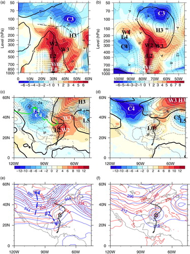
To illustrate the advantage of the anomaly-based analysis over the traditional total-field-based analysis, a few comparisons are given. In a horizontal field such as in Fig. 2, three troughs (#2, #4 and #5) and a ridge (#3) in a total field (Fig. 2a) become easily identifiable into three anomalous low centres (L2, L4 and L5) and an anomalous high centre (H3) (Fig. 2c) after removing climatic height (Fig. 2b). The advantage is even more visible in vertical cross sections such as in Figs. 3 and 4. Figure 3a and c show the vertical-latitude cross sections of the total and climatic height and temperature while Fig. 3e is height and temperature anomalies along 75.75°W longitude (crossing the TC centre) at 0600 UTC 25 October 2012. Although the differences also exists if one carefully compares the total field (Fig. 3a) with the climatic field (Fig. 3c), the detailed structures of Sandy and other nearby synoptic systems are not obviously visible in the total field. However, they are clearly revealed in the anomaly-based field (Fig. 3e). For example, there is a negative centre (L0) of height anomalies near the 1000 hPa and a positive centre (W0) of temperature anomalies at 700 hPa over Sandy. Another pair of positive height anomalies (H1) at 150 hPa and positive temperature anomalies (W1) at 250 hPa is also found over Sandy. From the view of hydrostatic equilibrium, the positive temperature anomalies (W1) at 250 hPa should have negative height anomalies below it. It thermodynamically implies that the merger between anomalous warm centre W1 and the Sandy vortex favours the first intensification of Sandy. To the north (50°N) of Sandy, a positive centre (H3) of height anomalies is located around 300 hPa, which separates a positive centre (W3) of temperature anomalies below and a negative centre (C3) of temperature anomalies above. Similar features of total, climatic and anomalous fields can also be observed from a vertical-longitude cross section along 20.25°N. The vertical structures of height and temperature anomalies are clearly visible over Sandy (W0, L0, W1, H1 and C1) and to its west (L2, W2 and C2) in the anomaly-based field (Fig. 3f), but not in the total field (Fig. 3b). Figure 4 is another vertical-latitude cross section but crossing the mid–high latitude trough and ridge areas (along 50°N, cf. Fig. 2a) at 1800 UTC 27 October 2012. The vertical structures of the ridge (#3) and trough (#4) are opposite in the anomaly-based field in Fig. 4c: an upper anomalous cold centre (C3) and a lower anomalous warm centre (W3) are separated by a positive centre (H3) of height anomalies (mid-latitude ridge) over 60°–70°W centred at 200 hPa, while an upper anomalous warm centre (W4) and a lower anomalous cold centre (C4) are associated with a negative centre (L4) of height anomalies (mid-latitude trough) over 90°–105°W at 250 hPa. It has been verified that the height and temperature anomalies satisfy the hydrostatic equilibrium (Fig. 3e, f and 4c). Given these advantages, anomaly-based fields will be used and compared with total field in the next subsection.

Fig. 2 (a) Total height (black line, 10×10 gpm interval) and total temperature (red line, 4 K interval), (b) climatic height (black line, 10×10 gpm interval) and climatic temperature (red line, 4 K interval) and (c) height anomaly (thin solid and dashed black lines, 4×10 gpm interval) and temperature anomaly (shading with while line, 2 K interval) at 300 hPa at 0600 UTC 25 October 2012. The grey dashed line with the symbol ‘' is the best track of Sandy. The thick green line in (c) is the low centre track of anomalous vortex L4 with the current location (green spot). In (a), the heavy dashed-blue lines indicate three troughs (#2, #4 and #5) while a ridge and the tropical cyclones (TC) are indicated by #3 and #1, respectively. In (c), letters ‘H’ and ‘L’ indicate the positive and negative centres of height anomalies, and ‘W’ and ‘C’ are the warm and cold centres of temperature anomalies.

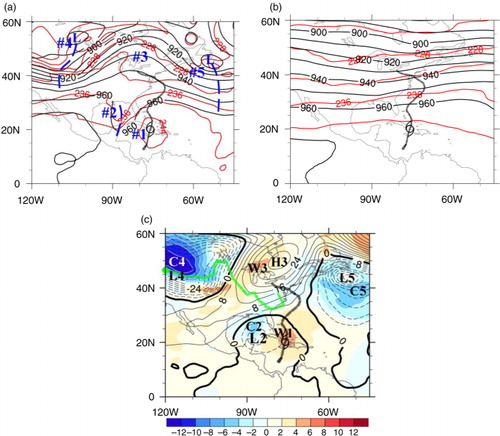
Fig. 3 Vertical-latitude cross sections of (a) total height (black line, 200×10 gpm interval) and total temperature (red line, 10 K interval), (c) climatic height (black line, 200×10 gpm interval), and climatic temperature (red line, 10 K interval) and (e) height anomalies (solid black line for positive and dashed black line for negative, 2×10 gpm interval) and temperature anomalies (red shading for positive and blue shading for negative with white line, 1 K interval), along 75.75°W longitude at 0600 UTC 25 October 2012. In (e), the dotted line indicates the axis of negative height anomalies, and the long-dashed line indicates the axis of positive height anomalies, while letters ‘H’ and ‘L’ denote positive and negative centres of height anomalies, and letters ‘W’ and ‘C’ denote positive and negative centres of temperature anomalies. Symbol ‘’ indicates the current position of Sandy. Panels (b), (d) and (f) are, respectively, the same as (a), (c) and (e), but for vertical-longitude cross sections along 20.25°N.

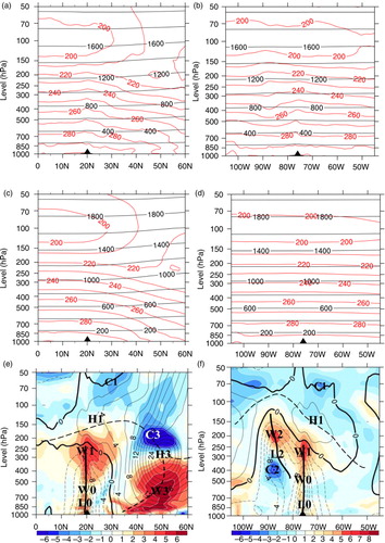
Fig. 4 Same as Fig. 3b, d and f but along 50°N at 1800 UTC 27 October 2012.

4.2. Structure evolution of Sandy

All the results in this subsection are obtained from the reanalysis data. When Sandy reached the strongest wind speed at 0600 UTC 25 October 2012, there were three major synoptic-scale systems (#2, #3 and #4 in Fig. 2a) which could potentially impact Sandy: a trough #2 to its west, a strong ridge #3 to its north and a deep trough #4 to its northwest over the central U.S. at 300 hPa. At this altitude, Sandy is not clear. As seen in the last subsection, these systems are well observed in the anomaly-based fields (Figs. 2c, 3e, 3f and 4c). For example, L0 and W0 reflect the lower-level structure of Sandy itself; L2, W2 and C2 reflect the trough #2; H3, W3 and C3 reflect the mid-latitude ridge #3; and L4, W4 and C4 reflect the mid-latitude trough #4. How these anomalous systems influence Sandy will be discussed in this subsection.

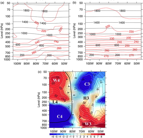
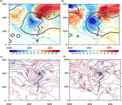
When Sandy headed northeastward on 27 October 2012, the anomalous vortex (L2 in Fig. 5c) moved eastward and merged into the Sandy vortex. This anomalous vortex appeared as a trough in the total field (#2 in Fig. 5e). The merger or combination of vortex L2 with Sandy (two low systems) deepened the TC vortex. This intensification can be observed from Sandy's maximum wind speed and central pressure in Fig. 1b. Meanwhile, an anomalous warm centre W3 below the mid-latitude anomalous high H3 in the upper troposphere and an anomalous warm centre W2 above the low L2 closed over the Sandy's vortex (Fig. 5a and b), which might be favourable to Sandy's intensification as a TC system. In this process, Sandy's warm core (W0) became indistinguishable from the two warm cores (W2 and W3) as they moved closer to it. This implies a thermodynamically favourable situation for its intensification under the hydrostatic equilibrium condition when warm centres closed at the upper troposphere. The anomalous low L4 over the Central United States was also approaching but still far away from Sandy (Fig. 5b–d). This anomalous vortex L4 is located at the upper troposphere (Fig. 5c) while the Sandy vortex L0 is observed in the mid–low troposphere (Fig. 5d). Unlike a typical TC, the original altitude of the warm core of Hurricane Sandy is limited to the lower layer while the storm size is large (Zhu and Weng, 2013). The height and temperature anomalies described above are not clear in the total-field synoptic charts as shown in Fig. 5e and f.

Fig. 5 Vertical sections of height anomalies (black solid and dashed lines, 2×10 gpm interval) and temperature anomalies (shading, 1 K interval) along (a) 75.75°W and (b) 30°N at 1800 UTC 27 October 2012, as well as the two horizontal synoptic charts of height anomalies (thin solid and dashed lines, 4×10 gpm interval) and temperature anomalies (shading, 2 K interval) at (c) 300 hPa and (d) 700 hPa, respectively. Panels (e) and (f) are the same as (c) and (d), but for total height (blue solid line, 8×10 gpm interval) and total temperature (red solid line, 4 K interval) at (e) 300 hPa and (f) 700 hPa, respectively. In (c), the thick green line is the low centre track of anomalous vortex L4 and the green spot is its current location. In (e), two blue dashed lines indicate the height troughs.

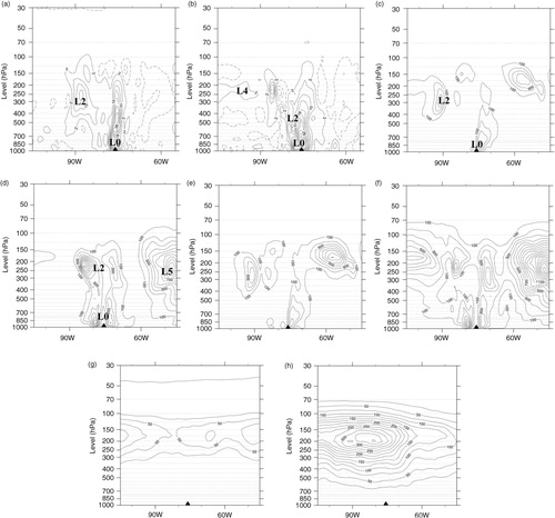
The combination process between the vortex L2 and the Sandy vortex L0 as well as the dynamical intensification of the Sandy vortex are clearly observed using vorticity anomalies and anomalous kinetic energy, respectively, from 0600 UTC 25 to 1800 UTC 27 October 2012 (Fig. 6). The two centres of vorticity anomalies in Fig. 6a and the two centres of anomalous kinetic energy in Fig. 6c represent vortex L2 and the Sandy vortex L0 at 0600 UTC 25 October. Two days later, the two centres, L2 and L0, were closely located, so the Sandy vortex had an intensification as indicated by the positive vorticity anomaly (L0+L2 in Fig. 6b) and the anomalous kinetic energy (L0+L2 in Fig. 6d) on 27 October. From 0600 UTC 25 to 1800 UTC 27 October 2012, anomalous kinetic energies increased from 124 to 1120 m² s⁻² at 250 hPa and from 430 to 815 m² s⁻² near 850 hPa over the Sandy vortex. This intensification process was not easily identified from the total kinetic energy (Fig. 6e and f). From Fig. 6e and f, several incomparable centres occurred due to increasing the climatic kinetic energy with increasing latitudes (Fig. 6g and h).

Fig. 6 Vorticity anomalies (8×10⁻⁵ s⁻¹ interval) along the zonal section crossing the centre of Sandy at (a) 0600 UTC 25 (75.75°W and 20.25°N), (b) 1800 UTC 27 (75°W and 30.75°N) October 2012. Panels (c) and (d) are the same as (a) and (b) except anomalous kinetic energy (100 m² s⁻² interval). Panels (e) and (f) are the same as (c) and (d) except total kinetic energy. Panels (g) and (h) are the same as (e) and (f) except climatic kinetic energy (25 m² s⁻² interval). Symbol ‘’ indicates the current position of Sandy. Capital letter ‘L’ indicates the position of vortex.

Sandy started to turn left at 0000 UTC 29 October. During the following 24 hours, Sandy experienced its third intensification when it was approaching the coastline. The vertical combination of the anomalous warm centre W3 in the upper troposphere and the anomalous vortex L4 in the middle troposphere was the primary reason for Sandy's pre-landfall intensification. After the turning point (0000 UTC 29 October, Fig. 7), interactions occurred among the anomalous low L4 in the middle troposphere, the anomalous high H3 in the upper troposphere and the Sandy vortex L0 in the mid–low troposphere. This will be confirmed by a set of BAMs in Section 4.3. At this moment, a positive centre and a negative centre of temperature anomalies are respectively located to the northeast and the west of Sandy (Fig. 7c). The anomalous cold centre C4 had not yet merged into the Sandy warm centre (W0) (Fig. 7d). Sandy cannot move northeastward, due to an anomalously strong blocking high to its northeast (Fig. 7a and c). The total height and temperature fields at 300 and 700 hPa cannot illustrate these relationships although the upper cold trough was visible to the west of Sandy (Fig. 7e and f).

Fig. 7 Same as Fig. 5 except for the vertical-latitude sections along (a) 71.25°W and (b) 33.75°N at 0000 UTC 29 October 2012, as well as the two horizontal anomaly-based synoptic charts on (c) 300 hPa and (d) 700 hPa, respectively. Total height and total temperature are shown at (e) 300 hPa and (f) 700 hPa.

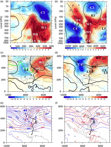
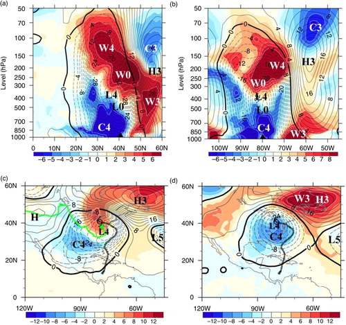
Approximately 5–6 hours before landfall (1800 UTC 29 October 2012), the anomalous low L4 with cold air mass intruded into the Sandy vortex from the southwest (Fig. 8e). Two vortices, L0 and L4, were experiencing a counterclockwise rotation. We will explain their interaction by our simple model in the next subsection. The Sandy vortex L0 moved northwestward and the anomalous cold vortex L4 moved southeastward, as illustrated by the two track lines in Fig. 8e. The anomalous vortex L4 was located in the upper troposphere (Fig. 8b and e) while L0 in the mid–low troposphere (Fig. 8b and f). Below the 250 hPa, an anomalous cold air column and an anomalous warm air column formed a strong contrast associated with three anomalous height systems (L0, L4 and H3) over the Sandy vortex (Fig. 8a and b). The anomalous warm air column was located over the Sandy vortex and there was an anomalous rising flow (green dashed line). The anomalous cold air column was observed beneath the anomalous low centre L4 and there was an anomalous sinking flow (green solid line). The anomalous rising and sinking branch flows should theoretically transform potential energy into kinetic energy. From 0000 UTC 29 to 1800 UTC 29 October, the central values of Sandy vorticity anomalies increased from 34×10⁻⁵ to 46×10⁻⁵ s⁻¹ near 850 hPa and the central values of Sandy anomalous kinetic energy increased from 1410 to 3100 m² s⁻² at 250 hPa and from 350 to 600 m² s⁻² near 700 hPa while the climatic kinetic energy increased from 380 to 530 m² s⁻² at 175 hPa over the Sandy vortex with increasing latitudes (figures not show). When vortex L4 captured Sandy's vortex (e.g. Fig. 9a and b), Sandy transformed into a large, intense extratropical cyclone. The strong gradient of pressure (geopotential height) was clearly observed in the northeast of Sandy (Fig. 9b). The enhanced energy resulted in an expansion of Sandy's wind field, which exacerbated the storm surge in her northeastern quadrant. In this process, the anomalous cold air mass cut the anomalously warm and moist air underneath and forced it to quickly ascend, which resulted in heavy snowfall in her southwestern quadrant. Again, the contrasts of positive–negative height and temperature anomalies are not clearly visible in the total-field-based analysis (Figs. 8c, 8d, 9c and 9d).

Fig. 8 Same as Fig. 5a and b except at 1800 UTC 29 October 2012 along (a) 73.5°W and (b) 38.25°N. Panels (c) and (d) are total height (black solid line, 200×10 gpm interval) and total temperature (red solid line, 10 K interval) at 1800 UTC 29 October 2012 along 73.5°W and 38.25°N, respectively. Height and temperature anomalies are on (e) 300 hPa and (f) 850 hPa at 1800 UTC 29 October 2012. In (a) and (b), the green solid and dashed lines, respectively, indicate anomalous descending and rising pressure velocities (10 hPa s⁻¹ interval).

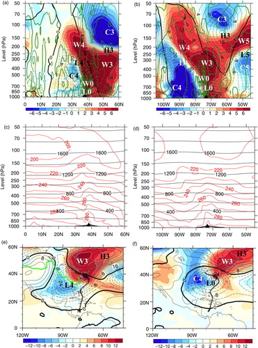
Fig. 9 Height anomalies (black solid and dashed lines, 4×10 gpm interval) and temperature anomalies (shading, 2 K interval) at (a) 500 hPa and (b) 850 hPa at 0000 UTC 30 October 2012. Panels (c) and (d) are the same as (a) and (b) but for total height (blue line, 8×10 gpm interval) and total temperature (red line, 4 K interval) on (c) 500 hPa and (d) 850 hPa, respectively.

At 0000 UTC 31 October 2012 Sandy had already moved inland. Figure 10 shows the post-landfall structure of height and temperature anomalies. In the vertical profile, two anomalous vortices L0 and L4 merged together into a common centre around 400–500 hPa, accompanied by two anomalous warm centres (W4 and W0) above and an anomalous cold centre (C4) below (Fig. 10a and b). This was a thermally stable structure with an anomalous warm layer above and an anomalous cold layer below during the day after Sandy's landfall as it reached the warm seclusion phase (Galarneau et al., 2013). At this moment, negative temperature anomalies were located over Sandy's vortex in the lower troposphere (Fig. 10d), while the upper troposphere was still covered by positive temperature anomalies (Fig. 10c).

Fig. 10 Same as Fig. 5a–d except at 0000 UTC 31 October 2012 for the two vertical sections along (a) 79.5°W and (b) 40.5°N, as well as the two horizontal anomaly-based synoptic charts on (c) 300 hPa and (d) 700 hPa, respectively.

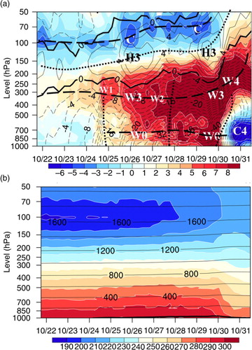
Figure 11a summarises the temporal evolution of the Sandy structure described by height and temperature anomalies during its lifetime. Following the TC centre, a time-pressure section of height and temperature anomalies can be depicted every 6 hours from 1800 UTC 21 to 1200 UTC 31 October 2012. Three major time points of intensification can be identified in Fig. 11a. The anomalous vortex of Sandy strengthened slowly from 21 October to early 24 October and its first rapid intensification occurred on late 24 October when the warm centre W1 overlapped the Sandy vortex vertically (the first vertical dotted line from the left). On 25 October, the intensity of Sandy weakened. A longer period of intensification occurred from 25 to 27 October when the anomalous centre L2 at 500 hPa with W2 and W3 at 300 hPa merged overlapping the Sandy vortex at 1800 UTC 27 October 2012 (the second vertical dotted line). The last rapid intensification of Sandy occurred from late 29 to early 30 October when the anomalous warm centre W3 at 300 hPa and negative height centre L4 at 350 hPa vertically combined with the anomalous warm centre W0 and negative height centre L0 of Sandy in the mid–low troposphere (the third vertical dotted line). Finally, an ET from a TC to an extratropical cyclone occurred when the anomalous vortex L4 (or the mid–high latitude trough in total field) merged into the Sandy vortex L0 in the mid–low troposphere on early 30 October. The cyclone occluded on 30 October when the anomalous cold vortex driven by the mid-latitude flow invaded the lower portion of the Sandy vortex. This evolution of the Sandy structure cannot be well illustrated from the total-field-based analysis. In Fig. 11b, no detailed evolution can be observed from the total height and total temperature following the Sandy centre from 1800 UTC 21 to 1200 UTC 31 October 2012 except a rapid decrease of temperature in the mid–low troposphere and a rapid increase of temperature from the upper troposphere to stratosphere after Sandy landfall. This is also a special case because most intense extratropical cyclones after ET processes move northward or northeastward (Harr et al., 2000). As previous studies indicated, TCs that undergo ET can produce strong surface winds and extreme rainfall that result in significant societal impacts (Thorncroft and Jones, 2000; Jones et al., 2003). The strong surface winds and extreme rainfall are largely contributed and analysed by the anomalous component in our method.

Fig. 11 (a) Time-pressure section of height anomalies (black solid line for positive and dashed line for negative, 2×10 gpm interval) and temperature anomalies (shading, 1 K interval) with 6-hour interval from 1800 UTC 21 to 1200 UTC 31 October 2012. The heavy dotted line and the heavy dashed line are the axes of height anomalies and temperature anomalies, respectively. Three vertical axes of height anomalies at the mid–low troposphere are indicated by the heavy dotted line at 1800 UTC 24, 1800 UTC 27 and 0000 UTC 30 October, respectively. (b) Same as in (a) except for total height (thin solid line, 200×10 gpm interval) and total temperature (shading, 10 K interval).

4.3. Model forecasts

The sudden left turn of Sandy occurred at the moment of 0000 UTC 29 October 2012 (Fig. 1a). We examine the Sandy track in the following 24 and 48 hours using a set of BAMs so finding the optimal level at 0000 UTC 29 October 2012. Figure 12 shows the meridional and zonal vertical distributions of vorticity anomalies crossing the centre of Sandy at 0000 UTC 29 October 2012. As an anomalous system, the vertical structure of Sandy was well described by the positive vorticity anomalies below 200 hPa with its maximum centre at about 850 hPa. In the north side of Sandy, a negative vorticity maximum was centred at around 50°N and 250 hPa, which corresponded to the anomalous high H4 (Fig. 12a). In the west side of Sandy, the positive centre of vorticity anomalies at 250 hPa over the US inland is the location of vortex L4 in Fig. 12b. At 1800 UTC 29 October, the two positive centres (L4 and L0) of vorticity anomalies merged together and intensified the Sandy strength (not shown).

Fig. 12 (a) Meridional and (b) zonal sections of vorticity anomalies (8×10⁻⁵ s⁻¹ interval) crossing the centre of Sandy at 0000 UTC 29 October 2012. Letters L0 and L4 indicate the locations of Sandy vortex and middle-latitude vortex, respectively. The 48-hour track forecasts of Sandy every 6 hours by (c) the GBAM, CBAM, ABAM and the results after removing other anomalous systems at 850 hPa as well by (d) classical BAMs initiated at 0000 UTC 29 October 2012. The black line with symbol ‘’ indicates the best track of Sandy in (c) and (d). (e) Time series of vorticity advection (blue dashed line, 10⁻⁸ s⁻²) by the climatic flow, vorticity advection (red line, 10⁻⁸ s⁻²) by the anomalous flow, and the beta term (purple line, 10⁻⁸ s⁻²) at 850 hPa.

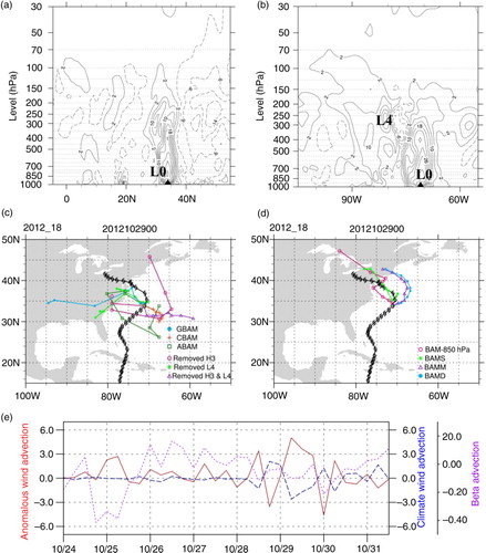
Using a set of BAMs, we examine the influence of climatic steering flow on the Sandy's track and the interaction among Sandy, H3 and L4 since 0000 UTC 29 October 2010. The optimal level is determined at 850 hPa with the maximum positive centre of vorticity anomalies (Fig. 12a and b). In Fig. 12c, the CBAM predicted that Sandy would head toward southeast in the following 24 and 48 hours; the ABAM predicted that Sandy will have a circular track in the coming 48 hours; and the GBAM showed that the 24-hour prediction is close to the best track. It can be easily understood that the predicted track of CBAM follows the climatic steering flow while the predicted track of ABAM is a result of interaction among three anomalous systems. If we only remove the anomalous low L4 from the GBAM, the predicted track is similar to that of the GBAM, which implies that the anomalous low L4 has little effect on the left turn of Sandy. The method of removing an anomalous system is simply to replace it by its climatic vorticity. For example, a positive anomalous vortex L4 is replaced by climatic vorticity. If we only remove the anomalous high H3 from the GBAM, the predicted track is a circle, which implies that the anomalous high H3 has an important role in the left turn of Sandy. If we remove the two anomalous systems of high H3 and low L4 all together from the GBAM, the predicted track is similar to that of the CBAM, which implies that the predicted track is basically influenced by the climatic steering flow.

We further examine the predicted tracks of three classical BAMs in Fig. 12d. If we use the BAM [eq. (10)] at 850 hPa, it predicts a reversed ‘z’ type track (BAM-850 hPa). Among the three classical BAMs, the best prediction is from the BAMS, because it captures the positive centre of vorticity anomalies in the lower troposphere. The other two models of BAMM and BAMD have larger track deviations from the best track, but their left turns are well predicted due to the influence of the high #3.

To physically and quantitatively detect the different impacts of the climatic flow and anomalous flow on the Sandy movement, a budget analysis is conducted. During Sandy's lifetime, most optimal levels are near 850 hPa as shown in Figs. 6a, 6b, 12a and 12b. The GBAM can be written as three terms as11

here, represents the vorticity advection by climatic flow, represents the vorticity advection by anomalous flow and is the beta term. Figure 12d compares the relative contributions of , and , respectively, to the moving direction and intensity of Sandy during its lifetime. We have calculated the three terms within the radius of 500 km and centred at the central point of Sandy. Results in Fig. 12e show that the beta term is so small that can be neglected. Since Sandy reached the hurricane intensity, its first peak at 0600 UTC 25 October was contributed largely by the vorticity advection by anomalous flow and the second peak from 0600 UTC to 1800 UTC 29 October was also largely contributed by the vorticity advection by anomalous flow. It implies that the vorticity advection by anomalous flow had a larger contribution to the intensity and motion of Sandy.

The results of the simple BAM experiment provide insight into the dynamics of the interacting anomalies and the influence of the climatic steering flow on Sandy's track. However, the GBAM cannot predict any TC tracks beyond 3 d because the optimal level is not constant and varies with time. On the other hand, the ECMWF model provided an excellent forecast of Sandy's landfall up to 8 d in advance at 0000 UTC 22 October 2012 (Bassill, 2014). Although the NCEP Global Forecast System (GFS) has a shorter predictability length than the ECMWF model, it also correctly predicted the landfall 4 d in advance at 0000 UTC 26 October 2012. The real-time forecasts from these two operational global models (ECMWF and NCEP GFS) will be investigated in a separate study with the following two issues: the comparison of Sandy's structure and intensity evolution from reanalysis data and the two operational models; and the examination of the possible reasons why the GFS had a shorter predictability length than the ECMWF model in Sandy's track forecasts.

5. Conclusion

An analysis approach based on anomalous field and a set of simple BAMs have been used to examine the structure evolution and unusual left turn of Hurricane Sandy (2012) before it made the landfall in the US east coast. The anomaly-based analysis can clearly (1) describe Sandy's vertical structure through the spatial configuration of height and temperature anomalies, and (2) reveal Sandy's intensity evolution including its dynamical and thermodynamical interactions with other synoptic systems, leading to the intensification and ET processes. The last intensification and the ET process occurred when the mid-latitude vortex (or the mid–high latitude trough in total field) merged into the Sandy vortex in the mid–low troposphere on early 30 October. At that time, Sandy transformed into a large, intense extratropical cyclone. During the ET process, an anomalous warm air column with an anomalous rising flow is located over the Sandy vortex and an anomalous cold air column with an anomalous sinking flow is observed beneath the mid-latitude trough. This process should theoretically transform potential energy into kinetic energy. The enhanced energy resulted in an expansion of Sandy's wind field, which exacerbated the storm surge in her northeastern quadrant. The anomalous cold air intruded into the southwest of Sandy and resulted in the heavy snowfall through upslope anomalous warm and moisture flow. A set of simple BAMs and the budget analysis of the vorticity advection confirmed the importance of the decomposition. The GBAM showed that the left turn of Sandy was mainly influenced by the anomalous high (blocking high) in its northeast.

6. Acknowledgments

We thank our three anonymous reviewers for their valuable comments and suggestions. We also thank Ms. Mary Hart of NCEP for her help to improve the readability of this manuscript. This research was supported by the National Natural Science Foundation of China (41375073) and the Key Technologies R&D Program (201306032).

Notes

¹Defined as the transition from a warm-core TC to a cold-core extratropical cyclone.

References

- Bassill N. P . Accuracy of early GFS and ECMWF Sandy (2012) track forecasts: evidence for a dependence on cumulus parameterization. Geophys. Res. Lett. 2014; 41: 3274–3281.
- Burger J., Gochfeld M. Perceptions of personal and governmental actions to improve responses to disasters such as Superstorm Sandy. Environmental Hazards. 2014; 13: 200–210.
- Chan J. C. L. , Gray W. M . Tropical cyclone movement and surrounding flow relationships. Mon. Weather Rev. 1982; 110: 1354–1374.
- Chen N. , Han G. Q. , Yang J. S . Hurricane Sandy storm surges observed by HY-2A satellite altimetry and tide gauges. J. Geophys. Res. 2014; 119: 4542–4548.
- Chen G., Sha W., Iwasaki T. Diurnal variation of precipitation over southeastern China: 2. Impact of the diurnal monsoon variability. J. Geophys. Res. 2009; 114 D13103. DOI: http://dx.doi.org/10.1029/2009JD012181.
- Crawford K. C. , Hudson H. R . The diurnal wind variation in the lowest 1500 ft in central Oklahoma: June 1966–May 1967. J. Appl. Meteorol. 1973; 12: 127–132.
- Galarneau T. J. , Davis C. A. , Shapiro M. A . Intensification of Hurricane Sandy (2012) through extratropical warm core seclusion. Mon. Weather Rev. 2013; 141: 4296–4321.
- George J. E. , Gray W. M . Tropical cyclone motion and surrounding parameter relationships. J. Appl. Meteor. 1976; 15: 1252–1264.
- Hall T. M. , Sobe A. H . On the impact angle of hurricane Sandy's new Jersey landfall. Geophys. Res. Lett. 2013; 40: 2312–2315.
- Harr P. A. , Elsberry R. L. , Hogan T. F . Extratropical transition of tropical cyclones over the Western North Pacific. Part II: The impact of midlatitude circulation characteristics. Mon. Weather Rev. 2000; 128: 2634–2653.
- Huang J. , Du J. , Qian W. H . A comparison between a generalized beta-advection model and a classical beta-advection model in predicting and understanding unusual typhoon tracks in eastern China seas. Weather Forecast. 2015; 30: 771–791.
- Jarvinen B. R., Neumann C. J., Davis M. A. S. A tropical cyclone data tape for the North Atlantic Basin, 1886–1983: contents, limitations, and uses. 1984; 21. Online at: http://www.nhc.noaa.gov/pdf/NWS-NHC-1988-22.pdf NOAA Tech. Memo. NWS NHC 22, Coral Gables, FL.
- Jones S. C. , Harrb P. A. , Abrahamc J. , Bosartd L. F. , Bowyere P. J. , co-authors . The extratropical transition of tropical cyclones: forecast challenges, current understanding, and future directions. Weather Forecast. 2003; 18: 1052–1092.
- Knabb R. D. Hurricane Sandy: hurricane wind and storm surge impacts. Town Hall Meeting: Hurricane and Post-Tropical Cyclone Sandy: Predictions, Warnings, Societal Impacts and Responses. 2013; Austin, TX: AMS. Online at: https://ams.confex.com/ams/93Annual/recordingredirect.cgi/id/23245.
- Magnusson L. , Bidlot J. R. , Lang S. T. K. , Thorpe A. , Wedi N. , co-authors . Evaluation of medium-range forecasts for hurricane Sandy. Mon. Weather Rev. 2014; 142: 1962–1981.
- Malakoff D. , Pennisi E. , Stone R. , Underwood E . US hurricane scientists assess damage from Sandy's deadly punch. Science. 2012; 338: 728–729.
- Marks D. G . The Beta and Advection Model for Hurricane Track Forecasting. 1992; Washington, DC: NOAA Technical Memorandum, NWS NMC-70. 89.
- Qian W. H . Principle of Medium and Extended Range Weather Forecasts. 2012; Beijing: Science Press. 440.
- Qian W. H. , Jiang N . The global monsoon definition using the difference of local minimum and maximum pentad precipitation rates associated with cross-equatorial flow reversal. Theor. Appl. Climatol. 2015; 124: 883–901.
- Qian W. H. , Shan X. L. , Liang H. Y. , Huang J. , Leung C. H . A generalized beta advection model to improve unusual typhoon track prediction by decomposing total flow into climatic and anomalous flows. J. Geophys. Res. 2014; 119: 1097–1117.
- Qian W. H. , Yang S . Onset of the regional monsoon over Southeast Asia. Meteorol. Atmos. Phys. 2000; 75: 29–38.
- Qian W. H. , Zhang G. W. , Huang J . Intensity evolution of Typhoon Megi (2010) revealed from anomaly-based atmospheric variables. Meteorol. Mon. 2015; 41: 806–815. (in Chinese).
- Simpson R. H . Hurricane: Coping with Disaster: Progress and Challenges since Galveston, 1900. 2003; Washington, DC: American Geophysical Union.
- Thorncroft C. , Jones S. C . The extratropical transitions of hurricanes Felix and Iris in 1995. Mon. Weather Rev. 2000; 128: 947–972.
- Uccellini L. W. Introduction to Sandy and the major impacts. Town Hall Meeting: Hurricane and Post-Tropical Cyclone Sandy: Predictions, Warnings, Societal Impacts and Responses. 2013; Austin, TX: AMS. Online at: https://ams.confex.com/ams/93Annual/recordingredirect.cgi/id/23244.
- Velden C. S. , Leslie L. M . The basic relationship between tropical cyclone intensity and the depth of the environmental steering layer in the Australian region. Weather Forecast. 1991; 6: 244–253.
- Yu R. C. , Li J. , Chen H . Diurnal variation of surface wind over central eastern China. Clim. Dynam. 2009; 33: 1089–1097.
- Yu R. C. , Zhou T. J. , Xiong A. Y. , Zhu Y. J. , Li J. M . Diurnal variations of summer precipitation over contiguous China. Geophys. Res. Lett. 2007; 34: 223–234.
- Zhu T. , Weng F. Z . Hurricane Sandy warm-core structure observed from advanced Technology Microwave Sounder. Geophys. Res. Lett. 2013; 40: 3325–3330.