A multiple length scale correlation operator for ocean data assimilation

Abstract

Ocean data assimilation systems can take into account time and space scale variations by representing background error covariance functions with more complex shapes than the classical Gaussian function. In particular, the construction of the correlation functions can be improved to give more flexibility. We describe a correlation operator that features high correlations within a short scale and weak correlations within a larger scale. This multiple length scale correlation operator is defined as a linear combination of Whittle–Matérn functions with different length scales. The main characteristics of the resulting correlation function are described. In particular, a focus is given on features that might be of interest to determine the parameters of the model: the Daley length scale, the normalised spectrum inflexion point and the kurtosis coefficient.

The multiple length scale operator has been implemented in NEMOVAR, a variational ocean data assimilation system. A dual length scale formulation was tested in a one-year reanalysis and compared with a single length scale formulation. The results emphasise the importance of estimating with great care the factors used within the combination. They also demonstrate the potential of the dual length scale formulation, in particular through a decrease of the innovation statistics for salinity profiles. The dual length scale formulation is now operational at the Met Office.

• background error
• covariance
• correlations
• length scales
• diffusion equation, recursive filter
• kurtosis

1. Introduction

The dominant time and space scales in the ocean vary considerably. For example, the ocean near-surface can feature spatial scales from hundreds to thousands of kilometres, due to the influence of the atmosphere wind and heat fluxes. Smaller spatial scales of the order of tens of kilometres, due mainly to internal ocean processes, are also important for ocean forecasting. Representing small scales depends on the resolution of the ocean models and observations. In general, global ocean forecasting systems run models on a resolution from 1/4° to 1/12° (e.g. Tonani et al., 2015, and references therein). Higher resolutions are also available for regional systems. The ocean observations assimilated in these systems are distributed irregularly in space and time. Satellites have a good horizontal coverage, but can only observe the ocean near-surface. In situ measurements are available in the deep ocean but their horizontal coverage is much sparser.

To account for large and small scales separately, Li et al. (2015) developed a multi-scale three-dimensional variational data assimilation (MS-3DVAR) system. In this scheme, two background error covariance matrices are constructed, and the classical cost function is split into two parts. This scheme has been successfully applied in regional systems (Li et al., 2013; Muscarella et al., 2014). A similar scheme has been applied in a data assimilation system for hurricanes by Xie et al. (2011). Multiple scales can also be accounted for in the classical cost function by giving the background error covariance a complex shape. Modelling a correlation function that matches a set of criteria can be done in different ways and has been widely studied. For example, Hristopulos (2003) uses the so-called Spartan Gibbs random fields where parameters such as scale, shape and radius can be set up differently. Gaspari and Cohn (1999) and Gneiting (2002) use products of compactly supported functions. Linear combinations of Gaussian or second-order autoregressive (SOAR) correlation functions have been studied by Purser et al. (2003b), Ma (2005) or Gregori et al. (2008). In their system, Martin et al. (2007) combine a SOAR correlation function with a large scale associated with errors arising from atmospheric forcing fields, with another SOAR correlation function with a small scale associated with errors arising from internal dynamics.

To model the SOAR correlation functions, Martin et al. (2007) use a recursive filter (Lorenc, 1992; Purser et al., 2003a, 2003b). The recursive filter is based on physical-space models and can therefore conveniently take into account the complex boundaries that often define the domains in ocean data assimilation. The diffusion equation (Derber and Rosati, 1989; Egbert et al., 1994; Weaver and Courtier, 2001) falls into the same class of correlation models. Weaver and Mirouze (2013) show that solving the diffusion equation with an implicit scheme leads to modelling a special case of the Whittle–Matérn functions of order depending on the number of pseudo time steps. For example, in one dimension, two pseudo time steps yield a SOAR function, with the limiting case, when this number is large, being the Gaussian function. Mirouze and Weaver (2010) also show that more complex shapes, such as correlation functions with negative lobes, can be modelled by using a linear combination of diffusion operators.

In this article, we describe a multiple length scale correlation operator, which linearly combines two- or three-dimensional (2D or 3D) Whittle–Matérn correlation functions of different length scales to construct correlation functions with more complex shapes. The multiple length scale correlation operator has been implemented and tested in the global 1/4 ° NEMOVAR system (Waters et al., 2015) that constitutes the data assimilation component of the current Met Office operational Forecast Ocean Assimilation Model (FOAM) system (Blockley et al., 2014).

Section 2 gives an overview of the main features of the Whittle–Matérn correlation functions and shows how they are linearly combined to construct the multiple length scale correlation operator. In Section 3 and Appendices A and B, some particular characteristics of the resulting function are described. Results of numerical experiments are detailed in Section 4. A summary and some conclusions are then given in Section 5.

2. Multiple length scale correlation operator

In this section, we first recall the main features of the Whittle–Matérn family that will be used as components in the linear combination. We then show how to construct a multiple length scale correlation operator by associating several of these components with different characteristics, in order to obtain 2D and 3D correlation models with more complex shapes.

2.1. The Whittle–Matérn family

In Weaver and Mirouze (2013), a special focus is given on the d-dimensional correlation functions of the Whittle–Matérn family1 where L is a scale parameter, Γ(ν) is the gamma function, K _ν is the modified Bessel function of the second kind of order ν, and r=∣ x – x ′∣ is the distance between points x and x ′ in . They studied in particular the special case when ν=M–d/2, where M is an integer and M>1 for d=1 and M>2 for d=2 and 3. For d=1 and d=3, this special case (WMsp hereafter) leads to a correlation function, often called an autoregressive function, defined as the product of an exponential function with a polynomial in r of order M–(d+1)/2. The Daley definition of length scale (Daley, 1991, p. 110) is commonly used in oceanographic and meteorological data assimilation to characterise the spatial scale of a correlation function. The Daley length scale is a quantity that can be estimated from statistics of background error. The scale parameter L is related to the Daley length scale D through the relationship2 where ∇² is the d-dimensional Laplacian operator. The limiting case for large M and fixed Daley length scale corresponds to the Gaussian function , with .

The Fourier transform of the correlation function eq. (1) is given by3 where , and is the vector of the spectral wave numbers associated with x . When the correlation function eq. (1) is modelled through an implicit diffusion operator, is the normalisation factor to be applied in order to ensure that the maximum of the function is equal to 1 and is given by4 with5

2.2. Combining the components

Following Mirouze and Weaver (2010), let us consider a d-dimensional correlation function constructed by linearly combining P d-dimensional correlation functions given by eq. (1)6 where the factors are such that to ensure the maximum amplitude of the correlation function is equal to 1. Negative lobes can be modelled by allowing some parameters to be negative. 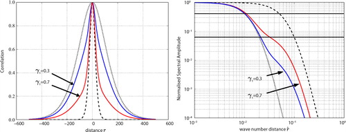In this case, however, some conditions on the parameters apply to guarantee f _d,P (r) to be a valid correlation function (Gregori et al., 2008). Figure 1 (left panel) shows the cross-section of an example of 2D correlation functions constructed from two correlation functions with a smoothness parameter ν=3 (d=2, P=2, M=4). The function c _2,1 (dashed black) uses a small-scale parameter of L ₁=10 grid points (D ₁=20), whereas the function c _2,2 (dotted black) uses a large-scale parameter of L ₂=50 grid points (D ₂=100). Two different linearly combined functions are presented: f _2,2 with (red) uses mainly the small-scale correlation function, and with (blue) uses mainly the large-scale correlation function. Both resulting functions retain the features of the small-scale correlation function for high correlation values, but show fatter tails that still allow for some correlation with more distant points. The transition occurs at medium correlation values and depends on the settings for (and ).

Fig. 1 2D correlation functions where the length scale parameters are L ₁=10 and L ₂=50 for c _2,1 and c _2,2, respectively, and ν ₁=ν ₂=3. The left panel shows a cross-section of c _2,1 (dashed black), c _2,2 (dotted black) and two different linearly combined functions: f _2,2 with (red), and with (blue). The right panel shows a cross-section at of their normalised spectrum. The black lines highlight the normalised spectrum values and . See text for details.

2.3. Combination using 1D components

When the hypothesis of separability holds, a d-dimensional correlation function can be split into 1D correlation functions for each axis (e.g. Stein, 1999, pp. 54–55 and references therein). Although this hypothesis is violated near coastlines, this method is convenient and hence often used to model the background error correlation function with the recursive filter or the implicit diffusion operator (Dobricic and Pinardi, 2008; Waters et al., 2015).

In eq. (6), the desirable correlation function is constructed from a linear combination of several different d-dimensional correlation functions. Each of these d-dimensional correlation functions can themselves be a product of 1D correlation functions. Another way of constructing a complex-shaped correlation function is to construct directly the d-dimensional correlation function as the product of 1D correlation functions, which are themselves a linear combination of 1D correlation functions with different characteristics. Equation (6) is therefore transformed as7

For example, a 2D correlation function constructed from three different length scales along the x-direction (dimension i=1) and two different length scales along the y-direction (dimension i=2) is denotedIn other words, several linear combinations are involved in the construction of the desirable correlation function eq. (7), whereas only one linear combination is required in eq. (6). Formulating a combination through eq. (7) rather than eq. (6) gives more flexibility because each direction can be shaped independently. However, this flexibility can translate into cumbersome square-root formulations, difficulties in the practical implementation and significant increase in cost. Therefore, the formulation from eq. (6) will generally be preferable.

2.4. Discretisation

In variational data assimilation, the cost function is generally minimised with a preconditioned iterative method (e.g. conjugate gradient). During the process, multiplications between the background error correlation matrix (or its square root) and a vector are required. In most cases, these products cannot be carried out directly because the background error correlation matrix is too large, so alternative approaches are needed.

A correlation operator is a symmetric and positive semi-definite application, which yields the convolution product of its kernel (a correlation function) with the initial condition it has been applied to. In a discretised representation, this convolution product is equivalent to the product of a correlation matrix, whose kernel is the discrete representation of the correlation function, with a vector representing the discretisation of the initial condition. Correlation operators based on a normalised recursive filter or a normalised diffusion operator are therefore widely used to simulate these products, once discretised.

In ocean applications, length scales are generally allowed to vary geographically. To be consistent and realistic, the factors should be allowed to vary geographically as well. Let us call F _d,P a correlation operator whose kernel is the multiple length scale correlation function given by eq. (6). When the factors are not constant, its kernel, centred at the point x ₀, is the solution of its application to an initial condition defined by a Dirac delta function centred at the point x ₀ and is given by8 At the point x ₀, the amplitude of eq. (8) is and is the maximum of the function as shown hereafter. Since c _d,p ( x − x ₀) is a valid correlation function, its maximum is at the point x ₀, that is, its first and second derivatives are 0 and <0 (negative), respectively, at the point x ₀. Assuming that is n times differentiable, the sum over P of the n ^th derivatives of is the n ^th derivative of the sum over P of , and hence is 0 since the sum of the factors is a constant function equal to 1. As a result, the first and second derivatives of eq. (8) at the point x ₀ are 0 and <0 (negative), respectively, defining thus the point x ₀ as the abscissa of the maximum. Therefore, the kernel of the correlation operator F _d,P is a valid correlation function, even when the factors are not constant. In this case, however, the kernel does not match exactly eq. (6). The distortion depends on the variation of the factors .

When the correlation operator F _d,P is discretised, its symmetry and positive definiteness can be guaranteed by constructing it as a product of ‘square-root’ factors9 where and C _d,P is a model of correlation functions of the form eq. (1) such as the normalised implicit diffusion operator or the normalised recursive filter. Γ _p is the diagonal matrix of the discretised factors associated with the correlation operator , and is such that , where I is the identity matrix. Square-root forms of the background error covariance matrix (and hence its correlation matrix) are needed for generating correlated noise in Monte Carlo applications, such as the randomisation method (Weaver and Courtier, 2001, and references therein) often used to calculate the normalisation factors. They are also used to precondition the cost function minimisation problem through the classical change of variable method (Lorenc, 1988; Courtier, 1997; Derber and Bouttier, 1999). However, when rectangular matrices are involved, like in eq. (9), using such a preconditioning increases the size of the minimisation vector. It is therefore preferable in this case to precondition the cost function using the full background error covariance matrix, as suggested in earlier studies by Derber and Rosati (1989) and more recently by Gratton and Tshimanga (2009) and Gürol et al. (2014). Both methods of preconditioning are equivalent and will lead to the same solution.

The calculation of the normalisation factors for the recursive filter or the diffusion operator is generally costly, and hence is an obstacle to the introduction of flow dependency into the correlation model. With the multiple length scale correlation operator, however, it is possible to obtain different shapes for the correlation function by using the same components C _d,P but with different factors . If these factors are computed at each assimilation cycle depending on characteristics of the flow and/or the observation network, flow dependency can be introduced into the correlation model without any extra cost, since the normalisation factors do not depend on .

3. Characteristics of the resulting correlation function

In this section, we explore the features of the correlation functions given by eq. (6). In particular, we focus on characteristics that might be of interest for defining the parameters of the model from an estimate of the desirable correlation function. In practice, the parameters of the correlation model are often estimated from, for example, an ensemble (Daget et al., 2009) or forecast differences (NMC method, Parrish and Derber, 1992) as done for the factors in our numerical experiment (see Section 4). For simplification, we are considering only constant length scales and in this section.

3.1. Daley length scale

From eq. (2), the Daley length scale of the resulting correlation function f _P (r) is given by10 When all P functions have the same smoothness parameter ν _p (M _p )=ν(M), eq. (10) reduces toIn the limiting case where M is large, the Daley length scales D _p are equal to the scale parameters , and the Daley length scale of the linearly combined function is given byIn the example of Fig. 1 (left panel), the Daley length scale of the functions f _2,2 and are D=23.7 and D′=34.9, respectively. These Daley length scales are much closer to the Daley length scale of c _2,1 (D ₁=20) than c _2,2 (D ₂=100) as can be clearly seen by comparing the distances when the correlation is between 0.6 and 0.7.

The Daley length scale allows the upper part of the resulting function to be characterised and hence provides a crude approximation of the smaller length scale involved in the linear combination. However, it fails to provide information on the tail of the resulting function.

3.2. Normalised spectrum

To characterise better the parameters of the model, it is worth studying its Fourier transform. From eq. (3), the normalised spectrum of the resulting function eq. (6) is given by11 where12 From eq. (4), when all P functions have the same smoothness parameter ν _p (M _p )=ν(M), we have and . Figure 1 (right panel) shows a cross-section at of the normalised spectrum for the previous 2D examples f _2,2=0.7c _2,1+0.3c _2,2 (red) and (blue). For small wave numbers, the resulting function is close to the large-scale function c _2,2 (dotted black), whereas for high wave numbers, it is closer to the small-scale function c _2,1 (dashed black). A transitional behaviour is observed in between which depends on the settings for (and ).

A noteworthy point of the normalised spectrum of a WMsp correlation function is given for the wave number distance . From eq. (3), we have

In the example of Fig. 1 (right panel), the thick black line at value 1/2 ^M =0.0625 crosses the functions and at wave number distances 1/L ₂=0.02 and 1/L ₁=0.1, respectively. However, the resulting function of the linear combination eq. (6) is not of the form of eq. (1). Therefore, the wave number distance cannot be defined by using eq. (2). Indeed, in our example, the Daley length scales of the linearly combined functions f _2,2 and are D=23.7 and D′=34.9, respectively. Using eq. (2) would give L=11.85 and L′=17.45, and hence, and , respectively. From Fig. 1 (right panel), it is clear that these wave number distances do not correspond to the normalised spectrum value 1/2 ^M =0.0625. An interesting consequence is that if the wave number associated with the Daley length scale through eq. (2) of a correlation function does not match the normalised spectrum value of 1/2 ^M , then this correlation function is not of the form of eq. (1). A linear combination of form eq. (6) might be required to approach its shape.

A second interesting point is given by the inflexion wave number that corresponds to the inflexion of the spectrum curve. Its calculation is given in Appendix A. From eq. (A2) of the appendix, the value of the normalised spectrum for the inflexion wave number is given byNote that this value depends on the smoothness parameter ν(M) and the dimension d of the correlation function, but not on the length scale parameter L. The inflexion wave number for the resulting functions of a linear combination is not trivial to derive from eq. (11). However, a correlation operator can be seen as a low-pass filter and the inflexion wave number as its cut-off wave number, that is, the wave number from which the filter starts to attenuate the signal. Because the behaviour of the resulting function of a linear combination is close to the larger scale function for small wave numbers (large scales), its inflexion wave number is expected to be approximately the same as the one of the larger scale function. Note that this closeness depends on the smoothness parameters ν _p (M _p ) and on the dimension d. This is illustrated in Fig. 1 (right panel) where both examples and are close to for the normalised spectrum value , highlighted by a thick black line. When all P functions have the same smoothness parameter ν _p (M _p )=ν(M), the inflexion wave number provides a crude approximation of the larger length scale involved in the linear combination.

3.3. Kurtosis coefficient

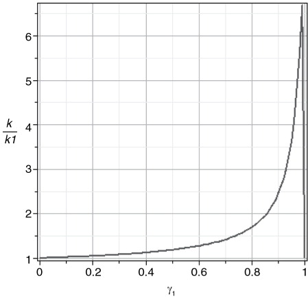
When the different length scales and smoothness factors involved in a linear combination are fixed, the possible resulting functions can still have very different shapes, depending on the factors used in the combination. In the example shown in Fig. 1 (left panel), the correlation function f _2,2 with has a sharper shape than with . The ‘peakedness’ or ‘tail fatness’ of a correlation function can be expressed in terms of the kurtosis (e.g. von Storch and Zwiers, 1999, p.32). Whereas the kurtosis of a fourth-order 2D WMsp function, such as c _2,1 and c _2,2, is k ₁=k ₂=3.86, the kurtosis of f _2,2 and are k=5.46 and k′=4.16, respectively, acknowledging their sharper shape. Figure 2 shows the evolution of the kurtosis ratio k/k ₁, calculated in Appendix B, for the correlation function f _2,2 with respect to . The higher , that is, the more the small length scale correlation function is involved, then the higher the kurtosis ratio is, that is, the sharper the resulting correlation function is. The ratio drops back to one abruptly when the factor is close to one. When all P functions have the same smoothness parameter ν _p (M _p )=ν(M), the kurtosis of the resulting correlation function provides some information on the factors used in the linear combination (see Appendix B).

Fig. 2 Evolution of the ratio k/k ₁ with respect to . k is the kurtosis of the 2D correlation function , with L ₁=10 and L ₂=50 for c _2,1 and c _2,2, respectively, and ν ₁=ν ₂=3. k ₁ is the kurtosis of the function c _2,1 (and c _2,2).

4. Numerical experiment

The multiple length scale correlation operator described in the previous sections has been implemented in the global 1/4°75 vertical levels FOAM system (Blockley et al., 2014). The FOAM system consists of the hydrodynamic model Nucleus for European Modelling of the Ocean (NEMO; Madec, 2008) coupled with the Los Alamos sea ice model (CICE; Hunke and Lipscombe, 2010) and the incremental first guess at appropriate time 3D scheme (Waters et al., 2015) of the variational data assimilation system NEMOVAR.

A numerical experiment was designed to assess the impact of the multiple length scale operator in a realistic framework and give insights on its potential. A one-year reanalysis has been run with the new correlation operator in a dual length scale formulation (hereafter DUAL experiment) in order to be compared with the original single length scale correlation operator (hereafter SNGL experiment). Both experiments start using the same initial states provided by the operational FOAM system (Blockley et al., 2014) on 4 August 2010. Each experiment is spun up for four months and the one-year period of interest runs from 1 December 2010 to 30 November 2011.

4.1. Assimilation scheme

Two cost functions are minimised separately in a one-day assimilation window: a sea ice cost function to assimilate sea ice concentration observations; an ocean cost function to assimilate satellite and in situ sea surface temperature (SST), temperature and salinity profiles from the EN4 data set (Good et al., 2013), and along-track sea-level anomalies. Both cost functions are minimised with 40 iterations of a B-preconditioned conjugate gradient algorithm (algorithm 2 in Gürol et al., 2014), where B is the background error covariance matrix. The ocean cost function accounts for multivariate variables through a balance relationship between the temperature (defined as a total variable) and the other variables (salinity, sea surface height, zonal and meridional components of current velocities) as described in Weaver et al. (2005). In the univariate problem that follows, spatial correlation matrices for temperature, unbalanced salinity and unbalanced sea surface height (SSH) are assumed to have a kernel of the form eq. (1). In the sea ice cost function, the sea ice concentration is considered as a total variable, that is, there are no balance relationships with any other variables, and its spatial correlation matrix is also assumed to have a kernel of the form eq. (1). The spatial correlation matrices are modelled by using 2D (unbalanced SSH and sea ice concentration) or 3D (temperature and unbalanced salinity) correlation operators constructed from a product of 1D normalised implicit diffusion operators.

4.2. Parameters of the correlation operator

The original correlation operator (SNGL) uses a single correlation function (no linear combination) for all variables. For temperature, unbalanced salinity and sea ice concentration, the horizontal length scales of the correlation functions are based on the first baroclinic Rossby radius, with a minimum of 25 km at high latitudes and a maximum of 150 km around the equator. For unbalanced SSH, the horizontal length scales are set to 400 km. The vertical length scales for temperature and unbalanced salinity are set to the mixed layer depth at the surface and decreased smoothly to reach a value of twice the vertical grid size at the mixed layer depth and below. This parameterisation allows for some flow dependency to be taken into account. However, it leads to non-trivial off-line calculation of the normalisation factors. A lookup table depending on a discrete set of possible mixed layer depths is then used to define the normalisation factors to apply at each grid point during the cycle (Waters et al., 2015).

For the dual length scale reanalysis (DUAL), the background error correlation functions for temperature and unbalanced salinity are constructed from eq. (6) with P=2. As in Martin et al. (2007), the linear combination associates a small scale to account for internal dynamics error and a large-scale for the errors arising from some atmospheric forcing fields. For the horizontal, the small scales are the same Rossby-radius-based length scales as in SNGL and the large scales are set to a constant value of 400 km. The choice of the second length scale was made according to the previous data assimilation system (optimal interpolation scheme) that was used in FOAM (Martin et al., 2007). For the vertical, the same parameterisation as in SNGL is used for both components.

Short tests of the dual length scale formulation were done by using constant factors and . Although the results show the potential of the multiple length scale operator, using constant factors was unsatisfying. Indeed, we expect the shape of the background error correlation function to be varying depending on the geographical location. Defining location-dependent factors is not trivial and is beyond the scope of this article. Therefore, we chose to use the factors defined from the seasonal variances calculated from the previous Met Office operational 1/4° system (Storkey et al., 2010) and interpolated in time.

The seasonal variances were calculated by fitting two SOAR functions to the correlations estimated from an ensemble of forecasts with different lead times (NMC method, Parrish and Derber, 1992). The forecasts were provided by the former Met Office operational system, where observations were assimilated through an optimal interpolation scheme. Because these variances are coming from a different system, they have been calculated according to different parameters. The small scale used to compute them was fixed to 40 km, whereas in our experiments it varies from 25 to 150 km depending on location. Moreover, the correlation functions modelled in our experiments are closer to the Gaussian function than the SOAR function.

For most of the ocean, the factor is about 0.25, that is, only weak correlations are spread further. In highly dynamic regions, such as the Gulf Stream, the Kuroshio or the Antarctic Circumpolar Current (ACC), this factor is increased to about 0.4. This increase is counter intuitive, since errors are expected to be relatively greater in the small scales for the strongly eddying regions. This is probably due to the method used to calculate the seasonal variances rather than being a genuine feature. The higher variance can be assimilated as a higher noise in the set of correlations points, and the fitting function method tends to over-estimate the larger scale in this case. At low SST (high latitudes), the factor is decreased to zero in order to use the small scale only near the ice edges (see Section 4.4 for more details).

4.3. An example of temperature increments

Figure 3 shows an example of temperature increments at the surface, obtained from the same initial states and the same set of observations. It represents the increments using the original formulation for the correlation operator as in SNGL (top left panel), and a dual length scale formulation as in DUAL (top right panel). The factor for the large scale of the surface temperature is illustrated in the bottom panel.

Fig. 3 Surface temperature increments on 1 December 2010 with the original formulation (top left panel) and a combination of two functions (top right panel) for the Gulf Stream region. The increments are calculated from the same initial states and the same set of observations. The factor defining the amount of the large scale to be used in the combination is shown on the bottom panel.

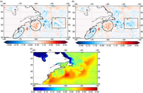
One can see that the increments are similar in both examples when the factor is small (northern and south eastern areas), although a slight smoothing effect can be observed for the increments provided by the dual length formulation. When the factor is larger, the spread of the innovations is visible for the increments of the dual length scale formulation. This is particularly noticeable for the cold increments along the coast between 30 °N and 42 °N (1), and for the warm increments around 60 °W (2). In the area around 42 °W and 45 °N (3), there is a gap in the cold increments for the original formulation, whereas in the dual length scale formulation, the fatter tails of the correlation function have filled the gap.

4.4. Sea ice concentration and SST increments conflict

During initial tests of the dual length scale formulation, a strong increase (17 %) was noticed in the innovation root mean square (RMS) of the sea ice concentration. This was caused by the large scale of the surface temperature spreading the innovations a long distance under the ice and conflicting with the sea ice concentration increments. When propagated by the model, the resulting analysis showed a less accurate daily mean field of sea ice concentration. Although the assimilation of sea ice concentration observations was working very hard on the next cycle to correct the field, it was constantly degraded by the SST increments.

To eliminate the problem, we redefine the factor for the temperature large scale such that it is reduced for low SST values. The large-scale factor at any depth is linearly interpolated from its current value to zero when the SST decreases from 3 °C to 1 °C and is maintained at zero when SST is below 1 °C. The small-scale factor is increased accordingly. In other words, the dual length scale formulation for temperature is smoothly replaced by the single length scale formulation at high latitudes near the ice edges. Using this new factor resolved the problem completely and led to similar sea ice concentration statistics for both single and dual length scale formulations. This ad hoc parameterisation should be revisited, however, when the factors will be tuned.

4.5. Innovations statistics

The assessment of the results is mainly based on innovation statistics, in terms of mean and RMS error (see Table 1). The innovations compare the observations before they are assimilated to their model counterparts. When they are not yet assimilated, the observations can be considered as an independent set of observations, and hence provide a useful diagnostic.

Table 1. RMSE for SNGL and DUAL in different areas

		RMSE
Variable	Area	SNGL	DUAL	%
SST in situ	Global	0.455	0.462	+1.5
	North Atlantic	0.516	0.527	+2.1
	Southern Ocean	0.468	0.484	+3.4
Temperature profile	Global	0.614	0.616	+0.3
	North Atlantic	0.812	0.806	−0.7
	Southern Ocean	0.568	0.565	−0.5
Salinity profile	Global	0.126	0.124	−1.6
	North Atlantic	0.218	0.214	−1.8
	Southern Ocean	0.108	0.103	−4.6
Mixed layer depth	Global	40.35	37.08	−8.1
	North Atlantic	44.13	42.94	−2.7
	Southern Ocean	63.76	56.44	−11.5
SSH	Global	0.071	0.075	+5.6
	North Atlantic	0.075	0.074	−1.3
	Southern Ocean	0.089	0.097	+9.0

The last column represents the normalised difference (DUAL–SNGL)/SNGL in percentage.

Globally, we note a slight increase of the RMS error of about 2–3 % in most regions with low variability for SST in situ innovations. In regions with higher variability such as the Gulf Stream and the ACC, this increase is even higher. A similar but lower increase can be seen in the SST innovations RMS error when the observations come from satellite. The results for temperature profile innovations are similar in both experiments, alternating slight decreases and increases. For salinity profile innovations, there is a general decrease of the DUAL RMS error. This decrease can reach more than 5 % in the South Atlantic and even more than 12 % in the Arctic Ocean and comes mainly from the first hundred metres. The mixed layer depth is derived from temperature and salinity profiles (Kara et al., 2000) and shows an interesting global decrease of 8 % for the DUAL RMS error. This probably results from a better salinity field in the top few hundred metres. A general increase of the RMS error for SSH innovations can be seen for DUAL, although there is a decrease in the Labrador Sea. The main increase is located in the Southern Ocean for the whole year. Highly dynamic regions, such as the Gulf Stream and the Kuroshio, also have slightly increased errors for DUAL. In both SNGL and DUAL, the background error correlation function for the unbalanced SSH variable is modelled through a single diffusion operator (no combination) with a constant length scale of 400 km. The SSH increment is then constructed using the unbalanced SSH increment and a baroclinic balance relationship based on the integration of the density increments (Weaver et al., 2005). The total SSH is thus affected by the changes introduced in the temperature and salinity increments by the dual length scale formulation. The decrease seen in the North Atlantic is possibly due to large-scale forcing dominating the Labrador Sea region during summer. More investigation is required, however, to determine more precisely the causes. In the Southern Ocean, eddies are particularly numerous and can extend quite deeply, affecting the isopycnals in such a way that they present steep gradients. A likely cause of the degradation is that the innovations are spread too far away by the large length scale, merging temperature or salinity increments belonging to different density layers. Solving this problem requires more complex strategies than the one adopted in Section 4.4

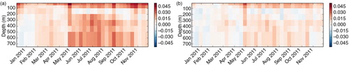
The main impact of the dual length scale formulation can be seen on the bias of the innovations. This is not surprising since the fat tails of the background error correlation functions account for large-scale errors and hence impact the error mean. The large scale of the dual length scale formulation is associated with the errors arising from some atmospheric forcing fields and its impact is therefore confined to the first 500 m. However, a slight impact can also be seen at greater depths in the Southern Ocean, possibly due to the high mixed layer depth in this region. Figure 4 presents Hovmoller plots for temperature innovation mean in the Southern Ocean. Near the surface, SNGL (left panel) shows a cold model bias during the summer that is mostly corrected in DUAL (right panel). Between 100 and 500 m, a warm model bias of about 0.2 °C can be clearly seen in SNGL during most of the year, except winter. The dual length scale formulation manages to reduce it, although a bias remains, in particular in January and February. Figure 5 shows Hovmoller plots for salinity innovation mean in the Southern Ocean. In SNGL (left panel), a fresh model bias can be seen in the first hundred metres for most of the year, except January. Another fresh model bias of about 0.03 also develops from the middle of autumn until the end of spring below 200 m. Both biases are well corrected in DUAL (right panel) although a small near-surface fresh bias remains for most of the year except summer.

Fig. 4 Hovmoller plots of the observation minus background innovation mean for temperature profiles for SNGL (left panel) and DUAL (right panel) in Southern Ocean. Blue colours denote a warm model bias, whereas red colours represent a cold model bias.

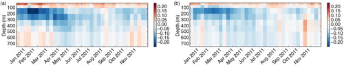
Fig. 5 Hovmoller plots of the observation minus background innovation mean for salinity profiles for SNGL (left panel) and DUAL (right panel) in Southern Ocean. Blue colours denote a salty model bias, whereas red colours represent a fresh model bias.

4.6. Results summary

The impact of a multiple length scale correlation operator for the background error was studied through one-year reanalyses. The aim of the experiment was to study the potential of a dual length scale formulation compared with the single length scale formulation that was currently used in the operational system.

Some issues arise, probably due to a lack of a proper tuning for the factors and . An increase of the RMS error for the sea ice concentration innovations was spotted and corrected by an ad hoc parameterisation of the factors before running the reanalysis. A general increase of the RMS error can be seen for SST innovations, possibly suggesting that the large length scale should be reduced in areas of dense observations. Regions of high variability are particularly affected because of the counter-intuitive increase of the factor in these regions (see Section 4.2). This is also the case for the SSH innovations. Moreover, the RMS error for the SSH innovations is particularly worsened in the Southern Ocean, probably due to the large length scale merging increments inappropriately. Some additional tests were performed, in which the large length scale was reduced at the edge of uncorrelated regions. These regions were identified by using horizontal gradients of the potential vorticity. These tests were reasonably successful at correcting the increase of the RMS for the SSH innovations and hence tend to confirm the hypothesis. We hope to develop this approach in future work.

Despite these issues, the potential of the dual length scale formulation was demonstrated. A large impact was seen on the innovation bias for temperature and salinity profiles, showing the usefulness of fatter tails in the background error correlation functions. The innovation statistics were also improved in terms of RMS for the salinity profiles and the mixed layer depth. The profile data performance was substantially improved in the Southern Ocean in particular, possibly at the expense of the SST and SSH performance. This trade-off was considered acceptable, however, for the dual length scale formulation to become operational. Further improvement is expected with carefully tuned factors and .

5. Summary and discussion

We presented a multiple length scale operator that linearly combines special cases of Whittle–Matérn correlation functions (WMsp) with different characteristics to obtain a correlation function with more complex shapes. Some features of the resulting correlation function, such as the Daley length scale, the kurtosis and the spectrum inflexion point, have been detailed. The multiple length scale operator can easily be implemented by modelling each of the WMsp correlation functions with a normalised implicit diffusion operator, for example. It can hence be used to model complex-shaped background error correlations in variational data assimilation systems.

The multiple length scale correlation operator has been implemented in NEMOVAR, an ocean 3D variational system, and a dual length scale formulation has been tested through a one-year reanalysis. When compared with a single length scale formulation, the results show an increase of the RMS error for innovations where a dense observation network is assimilated (SST and SSH). This suggests that the large length scale should probably be reduced in densely observed regions. The performance of profile data was improved in terms of innovation bias. The RMS error for the mixed layer depth and salinity profile innovations was decreased. These improvements justified an operational implementation in the Met Office system.

In order to set up this experiment, the factors and of the combination were defined from the seasonal variances calculated from the previous Met Office operational 1/4 ° system (Storkey et al., 2010). These factors define the amount of the small- and large-scale correlation functions, respectively, involved in the combination and hence define the shape of the resulting correlation function. The results of the experiment show a slight increase of the RMS error of the SST innovations and an increase of the RMS error of the SSH innovations in the Southern Ocean particularly. The worsening of the statistics might be due to the factors and not being properly tuned. The different experiments tested in this study showed that the results were sensitive to the choice of these factors. It is therefore important to define these factors accurately.

Defining good estimates of the factors and of the linear combination is a difficult task, beyond the scope of this article. The method of fitting functions that was used here requires an estimate of the resulting correlation function itself at each grid point. With the increasing resolution of the models, these estimates become more and more costly to calculate. Fitting specified functions to the resulting correlation function to determine the factors and is not flawless either. For example, the large-scale tends to be overestimated when the variance is high. Moreover, length scales are expected to vary depending on their location and to be anisotropic in some regions. This results in distortions of the resulting correlation function, which are not taken into account by the fitting function method. Overall, the method to estimate the factors and is not satisfying with respect to the importance of these factors. The technique using the kurtosis that we described in this article might be a good candidate for a more efficient method of estimation and needs to be studied further.

6. Acknowledgements

The authors thank CERFACS, ECMWF and INRIA/LJK who are collaborating to the development of the data assimilation system NEMOVAR. Funding support from the UK Ministry of Defence and the European Community's Seventh Framework Programme FP7/2007-2013 under grant agreement no. 283367 (MyOcean2) is gratefully acknowledged. We thank the anonymous reviewers for their helpful comments.

Notes

¹ Weaver and Mirouze (2013) show that correlation functions defined by eq. (1) can be modelled by applying M iterations of an implicit diffusion operator and normalising the result appropriately (see Section 2.4), in the special case when ν=M–d/2 .

²At a distance from the peak equal to the Daley length scale, the value of a Gaussian correlation function is . For the correlation functions in eq. (1), the Gaussian function is the limiting case when ν(M) is large. When ν(M) is small, a precise measurement is obtained by computing as given by eq. (1). In our example, this is 0.647. Note however, this is not exact for the resulting function f _d,P , although it is good enough for the purpose of a sanity check.

Appendix A

A.1. Inflexion wave number

In this appendix, we develop the calculation of the inflexion wave number for the normalised spectrum of the d-dimensional WMsp correlation function of form eq. (1). This distance represents the inflexion of the spectrum curve, that is, the cut-off of the low-pass filter defined by the correlation operator. It is calculated by finding the minimum of the normalised spectrum gradient and hence by nullifying the normalised Laplacian spectrum.

From eq. (3), the gradient of the normalised spectrum is given by the sum over d of its elementsA1

where , i=1,…, d is the i ^th element of the spectral wave number vector . The gradient of the normalised spectrum is negative for all wave numbers . Its value is for all () and for .

From eq. (A1), the elements of the Laplacian are given by

with i, j=1,…,d, and hence the Laplacian reads

The inflexion wave number is given by

If we assume that for all i, j, then we can rewrite the previous equation as

From there, we can define the (squared) inflexion wave numberA2

Appendix B

B.1. Kurtosis coefficient for the WMsp functions

The kurtosis describes the shape of a distribution, in particular its sharpness. For example, the kurtosis of a 1D normal distribution is k=3, whereas it is k=6 for a 1D exponential distribution, stressing the ‘peakedness’ of the latter. The kurtosis is defined as the normalised fourth moment divided by the normalised second moment squared. In this section, we calculate the kurtosis of the WMsp functions defined by eq. (1) and of the resulting functions of the linear combination eq. (6). We then show how the kurtosis can be used to provide information on the factors γ _p of a linear combination when the length scales are known.

From Gradshteyn and Ryzhik (2014), p. 685, eq. 6.561–16), the following results hold

and hence with a=1/L, we have

The WMsp function being even, we can then calculate the scaling factor for µ=v

where we used . The scaled second moment for µ=v+2 is

where we used . The scaled fourth moment for µ=v+4 is

where we used . The kurtosis for the WMsp function is then defined as

Note that the kurtosis depends on the smoothness parameter but not on the scale parameter. Indeed, the shape in terms of ‘peakedness’ of a WMsp correlation function depends on its order and its dimension only. However, the scaling factors and the moments involved in the calculation of the kurtosis do depend on the scale parameter. If the WMsp functions involved in the combinations are ordered such that L ₁<…<L _p , we can define α ₁=1<…<α _p such that L _p =α _p L ₁. When all the functions have the same smoothness parameter v _p =v, it is easy to see from the previous equations that N _p =α _p N ₁, and . Rearranging the equation of the kurtosis for the resulting function, we can define the ratioB1

where k ₁ is the kurtosis of the correlation function with the smallest scale parameter L ₁. In the particular case when P=2, the maximum of the ratio k/k ₁ is given for , and its value is

In the examples of Fig. 1, solving eq. (B1) with 0<γ₁<1, γ₂=1−γ₁ and α₂=5 leads to γ₁≈0.7 for k/k ₁=5.46/3.86≈1.41, and γ₁=0.3 for k/k ₁=4.16/3.36≈1.08.

References

- Blockley E. W. , Martin M. J. , McLaren A. J. , Ryan A. G. , Waters J. , co-authors . Recent developments of the Met Office operational ocean forecasting system: an overview and assessment of the new Global FOAM forecasts. Geosci. Model. Dev. 2014; 7: 2613–2638.
- Courtier P . Dual formulation of four-dimensional variational assimilation. Q. J. Roy. Meteorol. Soc. 1997; 123: 2449–2462.
- Daget N. , Weaver A. T. , Balmaseda M. A . Ensemble estimation of background-error variances in a three-dimensional variational data assimilation system for the global ocean. Q. J. Roy. Meteorol. Soc. 2009; 135: 1071–1094.
- Daley R . Atmospheric Data Analysis. 1991; Cambridge University Press, Cambridge.
- Derber J. , Bouttier F . A reformulation of the background error covariance in the ECMWF global data assimilation system. Tellus A. 1999; 51: 195–221.
- Derber J. C. , Rosati A . A global oceanic data assimilation system. J. Phys. Oceanogr. 1989; 19: 1333–1347.
- Dobricic S. , Pinardi N . An oceanographic three-dimensional variational data assimilation scheme. Ocean Model. 2008; 22: 89–105.
- Egbert G. , Bennett A. , Foreman M . Topex/Poseidon tides estimated using a global inverse model. J. Geophys. Res. 1994; 99: 24821–24852.
- Gaspari G. , Cohn S . Construction of correlation functions in two and three dimensions. Q. J. Roy. Meteorol. Soc. 1999; 125: 723–757.
- Gneiting T . Compactly supported correlation functions. J. Multivariate. Anal. 2002; 83: 493–508.
- Good S. A. , Martin M. J. , Rayner N. A . EN4: quality controlled ocean temperature and salinity profiles and monthly objective analyses with uncertainty estimates. J. Geophys. Res. Oceans. 2013; 118: 6704–6716.
- Gradshteyn I. S. , Ryzhik I. M . Table of Integrals, Series, and Products. 8th ed . 2014; Academic Press, San Diego.
- Gratton S. , Tshimanga J . An observation-space formulation of variational assimilation using a restricted preconditioned conjugate gradient algorithm. Q. J. Roy. Meteorol. Soc. 2009; 135: 1573–1585.
- Gregori P. , Porcu E. , Mateu J. , Sasvári Z . On potentially negative space time covariances obtained as sum of products of marginal ones. Ann. Inst. Stat. Math. 2008; 60: 865–882.
- Gürol S. , Weaver A. T. , Moore A. M. , Piacentini A. , Arango H. G. , co-authors . B-preconditioned minimization algorithms for variational data assimilation with the dual formulation. Q. J. Roy. Meteorol. Soc. 2014; 140: 539–556.
- Hristopulos D. T . Spartan Gibbs random field models for geostatistical applications. SIAM J. Sci. Comput. 2003; 24: 2125–2162.
- Hunke E. C. , Lipscombe W. H . CICE: The Los Alamos Sea Ice Model. 2010. Documentation and software users manual, Version 4.1 (LA-CC-06012), T-3 Fluid Dynamics Group, Los Alamos National Laboratory, Los Alamos.
- Kara A. B. , Rochford P. A. , Hurlburt H. E . An optimal definition for ocean mixed layer depth. J. Geophys. Res. 2000; 105: 16803–16821.
- Li Z. , Chao Y. , Farrara J. D. , McWilliams J. C . Impacts of distinct observations during the 2009 Prince William Sound field experiment: a data assimilation study. Cont. Shelf Res. 2013; 63: 209–222.
- Li Z. , McWilliams J. C. , Ide K. , Farrara J. D . A multiscale variational data assimilation scheme: formulation and illustration. Mon. Weather. Rev. 2015; 143: 3804–3822.
- Lorenc A. C . Optimal nonlinear objective analysis. Q. J. Roy. Meteorol. Soc. 1988; 114: 205–240.
- Lorenc A. C . Iterative analysis using covariance functions and filters. Q. J. Roy. Meteorol. Soc. 1992; 118: 569–591.
- Ma C . Linear combinations of space-time covariance functions and variograms. IEEE. Trans. Signal Process. 2005; 53: 857–864.
- Madec G . NEMO Ocean Engine. 2008. Note du Pole de modélisation No 27 ISSN No 1288-1619, Institut Pierre-Simon Laplace, Paris.
- Martin M. J. , Hines A. , Bell M. J . Data assimilation in the FOAM operational short-range ocean forecasting system: a description of the scheme and its impact. Q. J. Roy. Meteorol. Soc. 2007; 133: 981–995.
- Mirouze I. , Weaver A. T . Representation of correlation functions in variational assimilation using an implicit diffusion operator. Q. J. Roy. Meteorol. Soc. 2010; 136: 1421–1443.
- Muscarella P. A. , Carrier M. J. , Ngodock H. E . An examination of a multi-scale three-dimensional variational data assimilation scheme in the Kuroshio Extension using the naval coastal ocean model. Cont. Shelf. Res. 2014; 73: 41–48.
- Parrish D. F. , Derber J. C . The National Meteorological Center's spectral statistical interpolation analysis system. Mon. Weather. Rev. 1992; 120: 1747–1763.
- Purser R. J. , Wu W. S. , Parrish D. F. , Roberts N. M . Numerical aspects of the application of recursive filters to variational statistical analysis. part I: spatially homogeneous and isotropic Gaussian covariances. Mon. Weather. Rev. 2003a; 131: 1524–1535.
- Purser R. J. , Wu W. S. , Parrish D. F. , Roberts N. M . Numerical aspects of the application of recursive filters to variational statistical analysis. part II: spatially inhomogeneous and anisotropic general. Covariances. Mon. Weather. Rev. 2003b; 131: 1536–1548.
- Stein M . Interpolation of Spatial Data. Some Theory for Kriging. 1999; Springer, NewYork.
- Storkey D. , Blockley E. W. , Furner R. , Guiavarc'h C. , Lea D. , co-authors . Forecasting the ocean state using NEMO: the new FOAM system. J. Oper. Oceanogr. 2010; 3: 3–15.
- Tonani M. , Balmaseda M. , Bertino L. , Blockley E. , Brassington G. , co-authors . Status and future of global and regional ocean prediction systems. J. Oper. Oceanogr. 2015; 8: 201–220..
- von Storch H. , Zwiers F. W . Statistical Analysis in Climate Research. 1999; Cambridge University Press, Cambridge.
- Waters J. , Martin M. J. , Lea D. J. , Mirouze I. , Weaver A. T. , co-authors . Implementing a variational data assimilation system in an operational 1/4 degree global ocean model. Q. J. Roy. Meteorol. Soc. 2015; 141: 333–349.
- Weaver A. T. , Courtier P . Correlation modelling on the sphere using a generalized diffusion equation. Q. J. Roy. Meteorol. Soc. 2001; 127: 1815–1846.
- Weaver A. T. , Deltel C. , Machu E. , Ricci S. , Daget N . A multivariate balance operator for variational ocean data assimilation. Q. J. Roy. Meteorol. Soc. 2005; 131: 3605–3625.
- Weaver A. T. , Mirouze I . On the diffusion equation and its application to isotropic and anisotropic correlation modelling in variational assimilation. Q. J. Roy. Meteorol. Soc. 2013; 139: 242–260.
- Xie Y. , Koch S. , McGinley J . A space-time multiscale analysis system: a sequential variational analysis approach. Mon. Weather. Rev. 2011; 139: 1224–1240.