High-resolution precipitation re-analysis system for climatological purposes

Abstract

In this article, we describe the design and the validation of the Mescan precipitation analysis system developed for climatological purposes under the EURO4M project. The system is based on an optimal interpolation algorithm using the 24-h aggregated gauge measurements from the surface network. The background fields are the total accumulated precipitation forecasts at different resolutions from the ALADIN or HIRLAM mesoscale models, downscaled to 5.5 km grid spacing, chosen to match the time period of the climatological gauge reports. The validation of the Mescan system is carried out over the French territory employing various metrics and by providing forcing to a hydrological model to produce river discharges. The investigations have shown that the precipitation analyses have almost the same quality as the well-validated SAFRAN analysis system. In addition, the analysis of the precipitation variance spectra computed on the same horizontal domain has indicated that at short wavelengths the downscaled fields have significantly lower variability than a field produced by time integrating a forecast model. The Mescan precipitation analysis system has successfully been used to produce 24-h total accumulated precipitation re-analyses on a 5.5 km grid over Europe for the period 2007–2010.

• optimum interpolation
• limited area
• various background resolutions
• rain gauge data

1. Introduction

Among the meteorological variables, precipitation is of essential interest in weather forecasting and climate applications. It is also the most important one in hydrology, water management or agrometeorology. As such, long-term precipitation data sets have been produced by various large-scale global atmospheric re-analyses made available by leading meteorological centres such as NCEP-NCAR (Kalnay et al., 1996; Kistler et al., 2001), ECMWF (Uppala et al., 2005; Dee et al., 2011) and JMA (Onogi et al., 2005) (see Appendix A for the acronyms). Those re-analyses data spanning long time periods and different spatial scales have already proved their quality and usefulness in various research studies. However, they have been performed at horizontal grid spacing greater than 80 km that may be considered too coarse for applications used to examine weather variables over areas in which small-scale topographical influence and land-sea contrast are important. In addition, the accumulated precipitation fields are the result of a time-integrated forecasting model, the gauge measurements not being directly analysed by the data assimilation system.

A number of limited-area precipitation analysis systems based on the univariate optimum interpolation algorithm are described, for example, in Bhargava and Danard (1994), Häggmark et al. (2000), Mahfouf et al. (2007) and recently in Lespinas et al. (2015). Conceptually, the systems differ through the choice of the variable defined to carry out the analysis. Whereas Bhargava and Danard decided to carry out the analysis in the physical space on the precipitation value, in Häggmark et al. the variable is the precipitation value normalised by the standard deviation of the daily gauge measurements at the stations. A specific optimum interpolation analysis system, called SAFRAN, designed to provide forcing for an avalanche-forecasting model over French Alps is described by Durand et al. (1993, 1999). The design of SAFRAN makes it hardly portable over any other region outside France since it performs analysis of atmospheric variables on climatologically homogeneous areas of irregular shapes. A description of a modified SAFRAN version extended to cover France, together with some of its applications, is provided in Quintana-Seguí et al. (2008).

In all these approaches, the underlying principle consists of assuming that the precipitation and their associated errors are normally distributed both for background and observations. Assuming a log-normal distribution, Mahfouf et al. (2007) developed a precipitation analysis system in which the analysis is carried out on a transformed variable. This approach was also applied at ECMWF by Lopez (2011) in their 4D-Var data assimilation system. Recently, Lespinas et al. (2015) presented an assessment of the operational Canadian precipitation analysis system [initially developed by Mahfouf et al. (2007)] in which the analysis is performed on a cubic-root transformed variable as proposed by Fortin (2007).

In this article, we describe the Mescan precipitation analysis system designed and implemented as part of the EURO4M project, which was conceived to demonstrate the capacity of generating and providing reliable high-resolution gridded data sets of essential climate variables at the European scale. The Mescan analysis system has a wider range of options being capable to perform not only the precipitation analysis but also analyses of temperature and relative humidity at 2 m (Soci et al., 2013). The Mescan precipitation analysis system has been primarily designed to be run in a hindcast mode, for climatological purposes, but it can also be used for daily meteorological or hydrological operational activities. It has been developed to ingest 24-h accumulated precipitation data available in the long-term historical data sets from SYNOP and climate stations, which can be found in some European databases (e.g. ECA&D , ECMWF). At this development stage, it is not envisaged to use radar data in the system because these are neither long-term data nor covering whole Europe. Though the EUMETNET OPERA programme has expressed the endeavour to gather radar data across the western half of Europe, hard work has to be done in order to create reliable radar products that can be successfully used in data assimilation. In order to reach the demonstrative goal of the EURO4M project, 24-h accumulated precipitation re-analyses at 5.5 km grid spacing over Europe for the period 2007–2010 have been produced.

The article is organised as follows. Section 2 briefly describes the Mescan precipitation analysis system, the experimental setup together with the ensemble of the results and the methods used for the tuning of error statistics. Some aspects related to the high-resolution precipitation re-analyses at the scale of Europe are presented in Section 3, and a summary and the concluding remarks are provided in Section 4.

2. Precipitation analysis

This section provides a brief presentation of the optimum interpolation algorithm (Section 2.1) used as a tool to produce gridded analyses in meteorological data assimilation. A comprehensive description can be found, for example, in Lorenc (1981), Daley (1991) and Kalnay (2002). Also, in Section 2.1, some aspects of the Mescan system are briefly described. The experimental setup is presented in Section 2.2, while the validation is presented in Section 2.3. At the end of this section, we discuss some results related to the high-resolution precipitation analysis and spectral analysis.

2.1. Optimum interpolation

The optimum interpolation algorithm is generally derived, from a Bayesian perspective (Gelman et al., 1995), from the viewpoint of the minimum analysis error variance. It is a spatial interpolation algorithm that produces the best unbiased linear combination of observations with a first guess. Usually, the first guess, also called the background, is a short-range forecast from a numerical weather prediction model. The interpolation method is said to be optimal in the sense that it minimises the variance of interpolation errors if some hypotheses are verified, which includes knowing the error statistics of observations and background.

Let us denote the background by the vector of dimension N, the observation vector of dimension M and the analysis vector to be determined of dimension N. Let H be the observation operator that transforms the model forecast variable to the observation location, and be the background value interpolated at observation point j.

For a particular grid point i influenced by p nearby observations, the optimum interpolation analysis equation can be written as1

The difference is called the innovation (Talagrand, 1997), observational increment or background departure. The weights w _ij are found as the solution of the linear system (Kalnay, 2002, p. 160):2

where k=1, …, p. In practice, the system is solved for each analysis grid point by utilising a number of 16 nearby observations that lay within a radius of 200 km of the point of analysis. In eq. (2), B _jk and B _ik are the horizontal background error covariances between the observations points j and k, respectively, a model grid point i and an observation point k. R _jk is the covariance of the observation error between the points j and k. It is assumed that the background error correlation between two points is homogeneous and isotropic and also that the background and the observation errors are uncorrelated. Furthermore, under the hypothesis of uncorrelated observation errors, R become a diagonal matrix, . Here σ _o is the standard deviation of the observation error considered as the sum of the measurement and representativeness errors, and δ _jk is the Kronecker symbol. The representativeness error is caused by any physical scales, features or processes that affect the observation but are unresolved in the forecast model (Ingleby, 2015).

In the development of the Mescan precipitation analysis system described in this article, we have chosen to use the covariance of the background errors modelled by a second-order auto-regressive function as in Mahfouf et al. (2007), that for two points i and k is given by3

where σ _b stands for the standard deviation of background errors, r _ik is the distance between the points i and k on the same horizontal surface, and L is a characteristic horizontal correlation length scale. The background error covariances determine the spatial scales and the amplitude of the corrections applied to the background.

The Mescan precipitation analysis system is based on a two-dimensional univariate optimum interpolation method to perform the analysis in the physical space on the precipitation values, under the assumption that the errors associated with precipitation are normally distributed with zero mean and the error variances are for the observations and for the background.

Mescan is intended to be used in the EURO4M project to produce retrospective analyses that best fit the observations, not analyses for a numerical weather prediction system that generates the best subsequent forecast. To this aim, an important scalar is the ratio between the observation and the background error variances, . By tuning this parameter, the analysis can be forced to draw more closely to observations or to the background, respectively. Thus, for α=0, it is assumed that the observation is perfect, α=1, the observations and the background are supposed of the same quality, and for α>1, a higher confidence is given to the background.

The input observation data set to the analysis system is produced as an external pre-processing task to select the 24-h gauge measurements that match the time period of the climatological reports (06 UTC one day–06 UTC next day) and to remove duplicated reports from the same station. Once the input data set is ingested by the analysis system, an automatic quality control can be performed on the observations, innovations and departures from the analysis. A first task is done at the observation location in order to reject reports for which the difference in height between the model orography and the station altitude is greater than a specified value. The second task is to apply a statistical test to each observation, at each measurement point j, by comparing the normalised innovation with an assumed threshold, T, that is4

The default value for T is 10. The observation is flagged as: (1) correct if the ratio is below 0.7 times T, (2) suspicious if the ratio is between 0.7 times T and T, and (3) probably incorrect if it is greater than T. The final step of quality control is the consistency check (also called ‘buddy check’) where each observation is compared to the average of nearby observations within a circle of specified radius. At this stage, the observation receives the final quality control flag. Thus, some observations flagged as suspicious or probably incorrect at the previous step can be re-flagged as correct and admitted for analysis.

2.2. Experimental framework

To validate the Mescan precipitation analysis system, a set of experiments has been conducted in a hindcast mode over a domain covering France. The experiments are summarised in Table 1. One of the main arguments for performing the validation over the French territory has been the availability of the 24-h accumulated precipitation data from a high density gauge network. This network consists of 4300 stations (synoptic, automatic and climatological) from which about 1600 with reports sent on a daily basis and 2700 climatological stations with daily data available at the end of each month. Data from all these stations are quality controlled and then archived in the Météo-France Climatological database. However, the quality control does not provide an error-free data set. Though different types of errors (e.g. systematic errors due to the wind) are associated with the in situ precipitation measurements, this problem was not addressed in our study. Instead, we have considered that all measurement errors as well as representativeness errors are specified in the statistics of the observational errors. A comprehensive documentation of the various errors influencing the precipitation measurements is given in the WMO-8 guide, Chapter 6 (WMO, 2012). In the following, the set of the gauge measurements from 1600 stations with daily reports is denoted as the operational network, whereas the observation data set from the 2700 climatological stations not used in the production of the analyses is referred to as the independent observations and used to compute categorical scores. The precipitation data were taken from the Météo-France Climatological database and considered reliable and gross error-free. Thus, in the analysis system, the quality control of the observations was not applied.

Table 1. Summary of the experiments G1 and G2 performed for the evaluation of Mescan precipitation analysis system over the French territory

Experiment	Background fields	Error statistics
G1	– ALADIN forecasts at 5.5 km (native forecasts)	σ o=5 mm, σ b=13 mm, and L=35 km
	– Downscaled ALADIN forecasts from 9.5 to 5.5 km	idem
G2	– AROME forecasts at 2.5 km (native forecasts)	idem
	– Downscaled ARPEGE forecasts from 10 to 2.5 km	idem
EURO4M re-analyses	– Downscaled HIRLAM forecasts from 22 to 5.5 km	idem

A second argument was the presence of two high-resolution precipitation gridded data sets over France produced with SAFRAN and ANTILOPE operational analysis systems allowing inter-comparisons to assess the quality of Mescan analyses. ANTILOPE system (Laurantin, 2008) was developed at Météo-France to produce rainfall products over France at a grid spacing of 1 km, by combining radar and gauge data at a high temporal scale.

The set of experiments (henceforth named G1) includes analyses generated at 5.5 km grid spacing because this is the horizontal mesh size at which the EURO4M re-analyses were to be performed at the European scale (Fig. 1). The G1 experiments have been conducted in retrospective mode, for a trial period spanning 9 months (October 2009–June 2010). This period was chosen because the precipitation recorded at the surface encompassed a wide range of rainy systems from predominantly stratiform during the cold season (defined here as October–February) to mainly convective ones in the warm season (March–June).

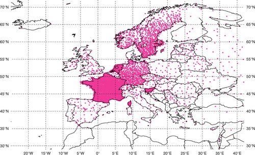
Fig. 1 EURO4M re-analysis domain and the spatial distribution of the 24-h precipitation observation network.

The analyses were produced over an area selected to be nested into the ALADIN-France domain, which was operationally used at Météo-France at the time of this work. ALADIN (Horányi et al., 1996) is a limited-area numerical weather prediction model developed within an international cooperation. The selected area consists of 288×288 points with a grid spacing of 5.5 km, centred at 46.2 °N and 2.2 °E. The ALADIN-France domain has 300×300 points with 9.5 km grid, centred at about 46.5 °N and 2.5 °E. The background is a 24-h total accumulated precipitation field initialised at 0600 UTC, downscaled from 9.5 to 5.5 km grid spacing through a 12-point cubic interpolation technique. By downscaling, a model field at coarse resolution is projected on a higher-resolution grid with the purpose of obtaining, as much as possible, more detailed information over a certain geographic area. The interpolation technique employed in our studies for downscaling purposes is the one developed in the ALADIN model and used operationally. Hereafter, the fields produced by downscaling will be denoted as the downscaled forecasts. For convenience we will refer to the forecasted fields performed at the higher-resolution grid (e.g. 5.5 km grid spacing) as the native forecasts. The 24-h total accumulated precipitation field is the sum of the four ALADIN model variables, that is, the stratiform and convective rain and snowfall amounts at the surface, respectively. The ALADIN model provides the snow field in terms of snow water equivalent. The background is chosen to match the time period of the climatological gauge reports issued daily, which are supposed to provide aggregated precipitation values from morning one day at 0600 UTC until 0600 UTC next day. It is considered that the model precipitation spin-up problem is reflected in the statistics of the background errors. The gridded analyses are generated at the resolution of the downscaled background, with observations ingested from the operational network. In the statistical model, constant values as in SAFRAN operational system were set up, as follows: the standard deviation of the observation errors, σ _o =5 mm, the standard deviation of the background errors, σ _b =13 mm, and the horizontal correlation length scale, L=35 km.

2.3. Validation of precipitation analysis system

A classical approach for validating an analysis is to apply different metrics to measure the fit to independent observations and to assess the skill. Henceforth, this method is referred to as the direct validation. A different approach is to use the analysis together with a set of other atmospheric variables, usually from a numerical forecast model, as initial data to force other applications such as a hydrological model to produce river flows or a surface model to simulate a number of surface variables (e.g. snow depth and soil moisture content). These derived output variables are then compared with the in situ measurements. We denote this approach the indirect validation.

We have performed direct validation for December, January and June and indirect validation for the entire period of 9 months (October 2009–June 2010).

2.3.1. Direct validations

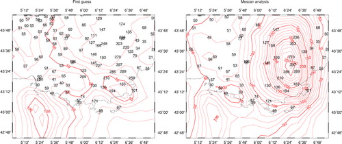
Primarily, we have tested the Mescan system for a severe weather event of 15 June 2010, when mesoscale convective systems caused, in the south-east of France, extremely large 24-h accumulated precipitation amounts. Figure 2 displays a zoom over the region of interest. In the left panel are overlapped all the available observations over that area and the background field, whereas the right panel illustrates the precipitation analysis and the observations from the operational network ingested in the analysis. Thus, two stations report amounts greater than 300 mm (with a peak magnitude of 397 mm in the Var county), 10 greater than 200 mm, and 23 raingauge values greater than 100 mm. Such high precipitation amounts, not unusual in the southern France and responsible for casualties and damages have an important societal impact despite being outliers from a statistical point of view. As such, even if the outlier is an accurate observation that contains small-scale information unresolved by the forecast model, it is usually rejected by the quality control of a data assimilation system. As shown in the left panel of Fig. 2, the operational ALADIN-France model at that time misforecasted the precipitation field both in location that is displaced by about 200 km to the south-west over the Mediterranean Sea and in maximum value (124 mm, hence of about three times lower than the largest measured value). Figure 2 (right panel) illustrates the ability of the Mescan system to represent this extreme event though the maximum value of the analysis is only 266 mm, which is about 33 % smaller than the highest rain gauge measurement. An examination of the innovations have shown values between −54 and 372 mm, the model value interpolated at the peak measurement location being of 25 mm.

Fig. 2 Maps of 24-h accumulated precipitation over the south-eastern France, valid at 0600 UTC 16 June 2010, for background (left panel) and Mescan analysis (right panel) with overlapped observations. Isohyets every 10 mm/24 h drawn for the background and analysis fields. Units mm/24 h.

The quality of the G1 analyses set is evaluated for December 2009–January 2010, a period encompassing several snowfall events, and for June 2010 when heavy precipitation affected mainly the south-eastern part of France. Over these periods, categorical scores have been computed using independent observations.

The skill of the precipitation analyses has been assessed at the same spatial scales using gridded observations, following a methodology described in Ghelli and Lalaurette (2000). Thus, the independent observations from the French network as well as the backgrounds, the Mescan and SAFRAN analyses have been projected onto a regular grid of 10 km. As a measure of skill, a number of standard categorical scores are computed (e.g. Heidke skill score, Frequency Bias Index, Equitable Thread Score, Probability of Detection, False Alarm Rate). A detailed explanation of such scores can be found in Jolliffe and Stephenson (2003) or Wilks (2006).

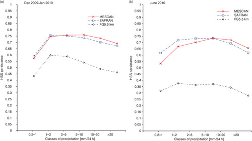
Figure 3 shows the monthly values of the HSS calculated against persistence as a function of classes of precipitation for the background (black dotted line), respectively, SAFRAN (blue dashed line) and Mescan (red solid line) analyses. The HSS ranges between −1 and 1, with one for a perfect analysis, zero for an analysis equivalent to persistence and for negative values the analysis is worse than the persistence. The persistence is the observation data set shifted in time by one day. It means that the gauge report from morning yesterday from each station was considered as if it were reported morning today, assuming that precipitation exhibits a statistical dependence in time. When examining the plots in Fig. 3a and b, it can be noticed that the quality of backgrounds changes with the season. Thus, the reduced skill in June (panel b) compared with December–January (panel a) highlights a known weakness of the sub-grid parametrisation of moist convective processes in the ALADIN model, common to other mesoscale models. That is, it produces too much precipitation when the small-scale atmospheric forcing is strong, particularly over the complex topography. Figure 3 also reveals the improved skill of the Mescan analyses compared to the background, which can be considered as a sanity check of the analysis system. Furthermore, when comparing Mescan and SAFRAN analyses, it appears that for precipitation classes greater than 5 mm, Mescan is slightly better than SAFRAN, whereas for lower values, SAFRAN has higher skill scores. The small difference between the scores of the two analyses illustrated in panel (a) can be related to the occurrence of the stratiform precipitation type in winter when the large-scale atmospheric forcing prevails.

Fig. 3 Monthly Heidke Skill Score against persistence computed as a function of classes of precipitation for (a) December 2009–January 2010, and (b) June 2010. Background (black dotted line), SAFRAN (blue dashed line) and Mescan (red solid line), respectively.

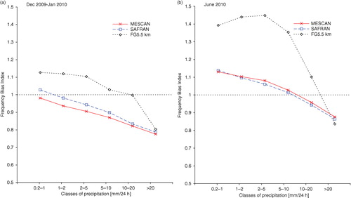
An important aspect of precipitation products to examine, particularly for hydrological applications, is their systematic errors. A common metric for such assessment, is the Frequency Bias Index (FBI) defined as a ratio between the frequency of forecasts and the frequency of actual occurrences of the event (Jolliffe and Stephenson, 2003). It ranges from zero to infinity. The optimal value for an unbiased forecast is one, whereas for values above (below) one, the model overestimates (underestimates) the precipitation frequencies.

A comparison between monthly FBI for the background, respectively, Mescan and SAFRAN analyses, computed as a function of classes of precipitation is shown in Fig. 4. In both panels, it can be noticed that the background (black dotted line) is biased and overestimates the precipitation up to the class 20 mm/day, particularly in June, and underestimates the larger amounts. The optimum interpolation algorithm should provide an unbiased analysis under the assumption that both the observations and the background are unbiased estimates. As the background is biased, the analyses away from the observations used to generate them may also be biased. While in Fig. 4a both SAFRAN and Mescan analyses are also underestimated, Fig. 4b reveals an overestimation of precipitation amounts for rates lower than 10 mm/day and an underestimation for higher rates. The discrepancy between the two analyses is small especially in June. Globally, over the 9 months period, the sum of the daily mean accumulated amounts are 705.9 mm for observations, 712.6 mm for Mescan and 723.2 mm for SAFRAN, demonstrating that overall Mescan is slightly less biased than SAFRAN.

Fig. 4 Monthly Frequency Bias Index computed as a function of classes of precipitation for (a) December 2009–January 2010, and (b) June 2010. Background (black dotted line), SAFRAN (blue dashed line) and Mescan (red solid line), respectively.

2.3.2. Indirect validation

An indirect validation of Mescan G1 precipitation analyses was carried out by using the hydrological ISBA-MODCOU system (Habets et al., 2008). ISBA (Noilhan and Mahfouf, 1996) is a land surface model that predicts surface energy budgets from an indirect atmospheric forcing. The input atmospheric variables for the ISBA model are temperature and specific humidity at 2 m, wind speed at 10 m, short- and long-wave incoming radiation fluxes and the precipitation flux (liquid or solid). The surface runoff and drainage fluxes provided by ISBA are used as input data to MODCOU (Ledoux et al., 1989) to simulate the temporal evolution of river flow (discharge) at the spatial scale of a river watershed. Aspects related to the calibration of MODCOU can be found in Golaz-Cavazzi et al. (2001) and Rousset et al. (2004). The validation of MODCOU river flow estimates is performed against measurements at the hydrological stations.

In order to generate MODCOU forcing, three experiments were conducted with ISBA by using a combination of atmospheric variables from different sources: (1) accumulated precipitation, incoming radiation and 10-m wind speed forecasted by the ALADIN model and Mescan analyses of temperature and relative humidity at 2 m (hereafter this experiment is referred to as ALADIN); (2) incoming radiation and 10-m wind speed from ALADIN and analyses of temperature and relative humidity at 2 m and precipitation from Mescan (experiment called Mescan); (3) SAFRAN analyses (SAFRAN experiment) in which all the input atmospheric variables necessary to run ISBA are produced by SAFRAN. The precipitation analyses are produced using observations from the operational network.

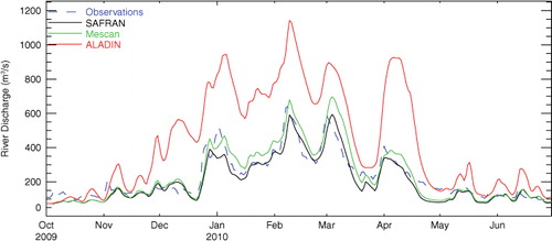
Figure 5 presents the daily river discharge of the Seine River observed at Paris-Austerlitz for the period October 2009–June 2010. The forcing from the ALADIN forecast model (red line) induces a large overestimation of the river flow, exhibiting high peaks with large discrepancies against observations, particularly at the beginning of January and February by 500 m³ s⁻¹, and April of about 700 m³ s⁻¹. On the other hand, Mescan (green line) and SAFRAN (black line) experiments show that, although peaks have a delay around 1 or 2 d, simulated river discharges follow very closely the observations. The comparison of ALADIN and Mescan curves reveals that the precipitation field is the main ingredient for estimating the Seine River flow. The Mescan analysis system clearly improves the quality of the forcing by correcting the known overestimation of the precipitation forecasts from the ALADIN model.

Fig. 5 Comparison of the time series (October 2009–June 2010) of daily river discharge for the Seine River at Paris-Austerlitz hydrological station.

In contrast with the Seine watershed, which is rather flat, the Rhône watershed contains large mountainous areas including part of the French Alps and Massif Central. This topographic feature enables the snow accumulation during the cold season. Examining the river discharges with various forcings for the Rhône River (Fig. 6), the difference between ALADIN (red line) and the other experiments is not as large as for the Seine River (Fig. 5).

Fig. 6 Comparison of the time series (October 2009–June 2010) of daily river discharge for the Rhône River at Beaucaire hydrological station.

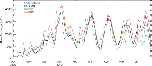
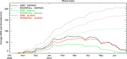
A comparison between Mescan (green line) and SAFRAN (black line) forcings shows similar results except at the beginning of May and during the month of June where the river flow derived with Mescan forcing is underestimated (Fig. 6). Figure 7 reveals that the underestimation of the river discharge by Mescan compared with SAFRAN is the result of a lower snowpack accumulation throughout the Rhône watershed. It can be noticed that at the beginning of January (February), the difference between the average accumulated snowfall produced by SAFRAN (black dotted line) and Mescan (red dotted line) is of about 42 mm (53 mm). Although seasonal cycle accumulation-melting occur, there is a large underestimation of the Mescan derived snow water equivalent field (green solid line) compared with ALADIN (red solid line).

Fig. 7 Comparison of the average accumulated snow water equivalent and snowfall over the Rhône River watershed for the period October 2009–June 2010.

This degradation can be explained by various factors that would need further investigation, such as the large discrepancy in mountainous areas between model orography and station height, large observation errors induced by non-heated rain gauges or blowing snow, incorrect specification of error statistics and correlation length scale.

Additionally, the 24-h precipitation analyses by Mescan are disaggregated into hourly precipitation with a phase change from rain to snow when the 2-m temperature is lower than 0.5 °C. The phase change introduces errors that can locally accumulate and become large particularly during the cold season. These errors affecting the snowpack accumulation in turn influence the river flow during the melting period.

2.4. Issues associated with the high-resolution analyses

An additional set of experiments (hereafter G2) has been performed at the 2.5 km grid spacing. The goal of the G2 is twofold: (1) to compare Mescan analyses with ANTILOPE precipitation products and (2) to assess the performance and to show the limitation of the Mescan precipitation system in the context in which further studies (or projects) might concentrate on the production of very high-resolution precipitation re-analyses by using observations from a surface network with low data density compared to the spatial scales resolved by the forecast model.

The background fields have been taken from two Météo-France operational models with contrasted horizontal resolutions, respectively, AROME-France and ARPEGE. The forecasts are initialised at 0600 UTC and cover 24 h such as to match the daily gauge measurement reports. AROME (Seity et al., 2011) is a limited-area convective permitting non-hydrostatic model integrated at 2.5 km grid spacing. ARPEGE is a global model (Courtier et al., 1991) run with a variable horizontal resolution which has a grid spacing of 10 km over France. Therefore, the background fields from ARPEGE have been downscaled from 10 to 2.5 km grid on the same domain as used by AROME. The 24-h accumulated precipitation analyses have been produced with observations from the operational network, for the cold season December 2013–January 2014 and also for the warm season June–August 2013. The error statistics and the correlation length scale are the same as in the G1 experiments.

The evaluation of the analyses from G2 experiments is similar to that from G1 experiments. Mescan analyses and ANTILOPE products were upscaled on a regular grid of 10 km. Likewise, the data from the 2700 independent stations were projected on the same regular grid and afterwards a number of categorical scores have been calculated. Figure 8a shows the HSS scores for the cold season, computed against persistence as a function of classes of accumulated precipitation. The skill of the two types of backgrounds is to some extent the same for precipitation in the range of 2–10 mm/day. For classes lower than 5 mm/day, the skill of AROME backgrounds is of about 3 % better than the downscaled ARPEGE forecasts, whereas for classes greater than 10 mm/day, in average there is an increased skill by about 5 % for ARPEGE. Same behaviour has been found for the warm season (not shown), except that the difference of skill between AROME and ARPEGE increases both for precipitation lower than 5 mm/day, to about 22 % for AROME side, and for precipitation greater than 10 mm/day, by about 26 % in average for ARPEGE. The decreased skill of AROME background compared with ARPEGE may arise from displacement and intensity errors, and does not convey a negative signal related to the overall performance of the model to forecast large amounts of precipitation. The small-scale patterns developed by AROME enhance the spatial variability at the observation location and may depict more accurately the overall precipitation system than ARPEGE, though, for example, it can miss the location of the precipitation maxima. The better skill in terms of HSS of ANTILOPE analyses compared with Mescan may indicate the beneficial impact of radar data in the very high-resolution surface analysis process. To improve the skill of the analyses performed using very high-resolution background fields, further work should concentrate, on one hand, on the tuning of error statistics and horizontal length scale and, on the other hand, on the usage of radar data in addition to the gauge measurements. The radar data are available at 1 km with spatial and temporal scales that are not represented in the background field. For this reason, a data upscaling work is necessary in order to create data at spatial resolution that provide useful information to the analysis system. The weather radar, however, does not measure precipitation directly, but reflectivity, which is a measure of the returned signal power, backscattered from the hydrometeors in an atmospheric scanned volume. The conversion from reflectivity to precipitation rate is done by making an assumption on the particle size distribution. It means that in addition to the gauge measurement errors, the analysis system has to account for the errors of the radar-derived precipitation data as well. The added value of assimilating radar quantitative precipitation estimates to produce 6-h gridded precipitation analyses is shown by Fortin et al. (2015).

Fig. 8 (a) HSS against persistence and (b) FBI as a function of classes of 24-h accumulated precipitation for December 2013–January 2014 for background fields from AROME forecasts (red dashed line) and downscaled ARPEGE forecasts (blue dashed line), ANTILOPE analyses (black solid line), analyses with AROME background (red solid line), analyses with downscaled ARPEGE forecast (blue solid line), respectively.

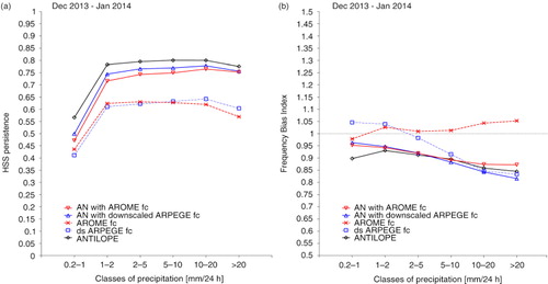
The plots in Fig. 8b, illustrating the FBI computed on the same regular grid of 10 km and using the same observation data set as for the HSS, reveal that while AROME exhibits an overall tendency to produce too much precipitation, the downscaled ARPEGE forecast fields underestimate the accumulated precipitation greater than 5 mm/day. It also appears that the precipitation analyses are all underestimated. The overall bias of Mescan analyses performed with AROME backgrounds is reduced compared with the ANTILOPE product. However, it is important to recall that the FBI is a measure of relative frequencies and not a measure of how well the analyses fit to the observations.

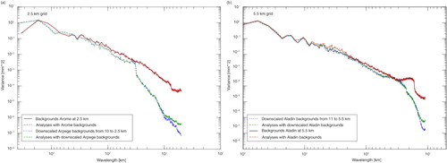
The presence of detailed small-scale spatial patterns is an important feature in high-resolution regional re-analyses compared with global re-analyses, which make them more suitable, for example, in hydrology and climate applications. Fine scales are developed by time integrating a high-resolution numerical forecast model. When employing a spatial interpolation method to downscale a prior atmospheric field from a coarse to a higher-resolution horizontal grid, spurious noise is introduced. We have quantified this noise by computing the variance spectra of the monthly mean 24-h total accumulated precipitation over the AROME-France domain at Δx=2.5 km, and over a much larger domain of 1080×1000 points with 5.5 km grid spacing covering Europe, set up at Météo-France to produce re-analyses under the EURO4M project. Variance spectra were computed based on an algorithm that employs a discrete cosine transform, proposed by Denis et al. (2002).

Figure 9a and b displays the variance spectra of the monthly mean 24-h total accumulated precipitation fields for December 2009. In both panels, it can be noticed that at the shortest wavelength represented in the model, that is, 2 Δx, the variance of the downscaled forecasts is significantly lower than the variance of the native forecasts. There is also a steep decrease of the variance at the wavelength corresponding to 3 Δx for native forecasts. As explained in Ricard et al. (2013), the reduction in the spatial variability comes from the quadratic truncation applied to the model orography. Furthermore, Fig. 9a shows that such a decrease is also triggered in the downscaled fields at about 12 Δx, corresponding to three times the value of the coarser ARPEGE grid, that is, the decrease of the variability begins below 3 Δx of the input grid. This finding may indicate that the decrease of the variability is triggered at the wavelength corresponding to the quadratic truncation applied to the input model orography. The precipitation analysis increases the variance at short wavelengths when the background is a downscaled forecast (dashed green line) and has a rather neutral impact when it is performed with background from a native forecast (dashed red line). Note that the black solid line and the red dashed line overlap. The effect of the analysis is to modify the mean value of the precipitation field. Same results have been obtained for the month of June 2013 (not shown). These findings show that for applications in which the small-scale spatial variability is important (e.g. in hydrology), it is more desirable to run a high-resolution model than to downscale fields employing the 12-point cubic interpolation technique, particularly when there is a large difference between the initial and the final grid resolutions. An alternative downscaling method, such as the statistical downscaling using regression models, that potentially may improve the quality of the background, may not generate physically consistent small-scale features. Indeed, Fowler et al. (2007) noted that in comparison to the dynamical downscaling, the statistical methods tend to underestimate variance and poorly represent extreme events.

Fig. 9 The variance spectra of the monthly mean 24-h total accumulated precipitation as a function of wavelength computed on (a) AROME-France domain at 2.5 km grid (for January 2014), and (b) a domain for running ALADIN model at 5.5 km grid covering Europe (for December 2009). The blue dotted lines stand for the downscaled forecast fields, the green dashed lines for the analyses performed with downscaled fields, the black solid lines for native forecasts at 2.5 km (5.5 km) grid and the red dashed lines correspond to the analyses performed with backgrounds from native forecasts. Note that the scales of the abscissa differ in (a) and (b).

The added value of using a background field from a high-resolution native forecast instead of downscaled one is shown in the spectral analysis but is hidden from the categorical scores without using a denser observation network. In order to demonstrate the better skill of forecasts at 2.5 km grid spacing, non-traditional verification methods such as the fuzzy techniques are required (Ebert, 2008; Amodei and Stein, 2009).

2.5. Estimation of error statistics

The goal of this section is to describe the tuning of the horizontal correlation length scale and the estimation of error statistics which have been performed based on the hypotheses of homogeneity and isotropy. The standard deviation of background and observation errors is estimated under the assumption of optimality, following the a posteriori diagnostic approach proposed by Desroziers et al. (2005).

2.5.1. Correlation length scale

The NMC method (Parrish and Derber, 1992) provides a pragmatic formulation to compute the background error covariance matrix using the forecast error statistics deduced from lagged forecasts valid at the same time. In order to estimate the statistics of background errors, we have considered differences of 24-h accumulated precipitation forecasts from ALADIN-France downscaled at 5.5 km, lagged by 12 h, as follows:

• fc -fc denoted as F ¹;

• fc denoted as F ²;

where ‘fc’ stands for the forecast, the subscripts indicate the starting day ‘d’ of the forecast and the superscripts indicate the hour of model initialisation plus the forecast range.

The background errors are computed at each grid point i as ɛ _i = F– F, for pairs of rainy points, when both F andF are greater than 0.01 mm. The horizontal covariance at distance r is estimated by employing the relation in Mahfouf et al. (2007):5

where N(r) corresponds to the number of independent pairs of points i and j separated by distance r, and is the mean error. The separation distance is binned in 10 km intervals from 0 to 600 km.

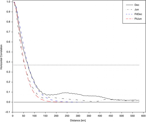
The horizontal correlation lengths for precipitation, for the whole month of December 2009 and June 2010, are presented in Fig. 10. Using the least-square method and the function defined in eq. (3), the best fit for December (blue curve) and June (red curve) is estimated for L=32 km and L=24 km respectively. We assume that these results are generally valid for the cold and warm seasons. The distances from which the correlations decrease by a factor of e ⁻¹ are 69 km for December and 52 km for June. It should be noticed the tendency towards larger correlation lengths during the cold season when stratiform precipitation prevail than in summer when convective precipitation dominate. In addition, the curves show that the correlation decreases below 0.1 for a separation distance greater than 150 km.

Fig. 10 Horizontal correlation lengths for precipitation determined in ALADIN-France domain with the ‘NMC method’ for December 2009 (black solid line) and June (black dashed-dotted line). The best fit for December (blue short-dashed line) and for June (red long-dashed line) are derived with L=32 km and L=24 km respectively. The horizontal dotted line depicts c⁻¹.

The standard deviation of background errors was computed from the statistics of ɛ leading to the value of 4.05 mm for December and 5.41 mm for June. Under the hypothesis of uncorrelated background and observations errors, the standard deviation of observation errors, σ _o , can be estimated from the variance of the innovations producing for December (June) a value of 1.97 mm (3.42 mm).

2.5.2. A posteriori diagnostic of error statistics

Desroziers et al. (2005) provide a diagnostic method to estimate error statistics in observations space, under the hypothesis that the observation and background errors are uncorrelated. Based on innovations, one can check that assuming that σ _o and σ _b are correctly specified in the analysis. Here E[ ] is the statistical expectation operator, O stands for the vector of observations, F is the vector of the background values interpolated to the observation locations and T for the transpose of the vector. The observation and the background variance errors can be estimated from and , where A is the vector of analysis values at observation locations.

We have used the computed innovations and analysis departures from the analyses performed at 5.5 km grid, with observations from the operational network, for the month of December 2009 and June 2010. From the a posteriori diagnostics, the estimated values of standard deviation of observation and background errors for December (June) are σ _o =2.35 mm (4.19 mm) and σ _b =4.49 mm (6.98 mm), respectively. Since the initial values used in the Mescan system are σ _o =5 mm and σ _b =13 mm, it appears that both of them are largely overestimated for December.

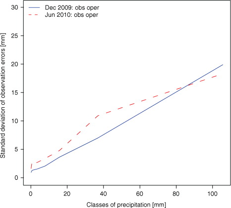
The same methodology was applied to estimate the standard deviation of observation errors as a function of classes of accumulated precipitation. The results are plotted in Fig. 11. Both curves illustrate that the observation errors exhibit a growth related to the amount of the daily precipitation, and hence, they can be approximated by a linear function of the form σ _o (x) = ax+b, x being the measured value, with a and b constants. The curves indicate that the standard deviation of observation errors may reach 20 % of the measured value in December (blue line) and around 30 % in June (red dashed line) for precipitation by 40 mm/day. These plots suggest that the usage of a variable σ _o in the analysis system can be more appropriate than to assign it a constant value. The choice for a variable σ _o may also be justified, for example, by an increase of the measurement errors during heavy precipitation episodes associated with strong wind gusts. At the same time, employing a variable σ _o implicitly leads to a discussion about specification of σ _b . Thus, a too high value of σ _b such as to ensure σ _o (x) < σ _b for all precipitation classes will rather neglect the background and draw the analyses too much to the observations, particularly for light precipitation which in turn are not very accurate either. A more straightforward approach is to consider σ _o (x) as a sort of step function and to assign it an upper limit: σ _o (x) = ax+b, for x<d and : σ _o (x) = c, for x≥d, where c and d are defined constant values. In such a way, σ _b could be given a value estimated by the a posteriori diagnostic.

Fig. 11 Standard deviation of observation errors as a function of classes of 24-h accumulated precipitation amount in the observation space for December 2009 (blue solid line) and for June 2010 (red dashed line).

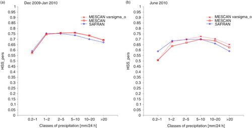
Figure 12 shows that for both trial periods there is an improvement of the skill, in terms of HSS against persistence, of the analyses produced with a variable σ _o . In that case, we have chosen σ _o =0.1 x+0.9. Except for precipitation amounts lower than 2 mm/24 h, in both panels the scores of Mescan with variable σ _o (red dotted line) are better than SAFRAN (blue dashed line) and Mescan with the constant σ _o =5 (red solid line).

Fig. 12 Monthly Heidke Skill Score against persistence computed as a function of classes of precipitation for (a) December 2009–January 2010, and (b) June 2010. SAFRAN (blue dashed line), Mescan (red solid line) with constant σ _o , and Mescan with variable σ _o (red dotted line), respectively.

3. Aspects related to the precipitation re-analyses at the European scale

Among other things, the EURO4M project allowed close cooperation between several National Meteorological Services. This was the case between SMHI and Météo-France. Intensive collaborative work was necessary to create background fields and common observation data sets. In this section, we briefly describe the input data used to produce the 4-yr data set of 24-h accumulated precipitation re-analyses at 5.5 km over Europe for the period 2007–2010. In addition, we emphasise some difficulties encountered with the precipitation observations. The European gridded precipitation re-analyses have been produced using the same error statistics as in the G1 and G2 experiments (i.e. σ _o =5 mm, σ _b =13 mm, and L=35 km).

3.1. Background fields

The background fields for 24-h precipitation analyses at the European scale come from the HIRLAM forecasts initialised at 0000 and 1200 UTC from a 3D-Var re-analysis performed by SMHI. The background field is downscaled from 22 to 5.5 km and is created as the sum of 12-h accumulated precipitation: (fc ^00UTC+18-fc ^00UTC+06)+(fc ^12UTC+18 -fc^12UTC+06), where ‘fc’ denotes the forecast and the superscripts indicate the hour of the model initialisation plus the forecast range. A combination of forecasts of different ranges has been successfully tested in Mahfouf et al. (2007). To reduce the model spin-up problem, they selected the precipitation fields not too close from the initial time, but not too far either such as to have a good evolution of the large-scale fields.

3.2. Observations

A challenge for producing long-term precipitation re-analyses at the European scale is the availability of observations from a relatively dense gauge network. For example, it has been found that the observation density from the operational archive of ECMWF or Météo-France received on the GTS is low. Particularly, the mountainous areas are poorly sampled and large regions such as southern and eastern Europe have sparse data (as illustrated in Fig. 1). After investigations, it has been decided to use observations from ECMWF and ECA&D (version 6) databases. Prior to creating the input observation data set for the Mescan system, a data pre-processing work has been carried out, primarily to select only 24-h precipitation reports that match the climatological day. First the data have been merged and then the duplicated reports discarded. Finally, additional observations from the Swedish and French national networks were added. A particular attention was given to the ECA&D database which has been designed for climatological purposes (rather than for data assimilation). This archive contains data from a number of n stations (divided into the same number of individual files) across Europe, not all of them received on the GTS, each station having its own data available as a time series of daily datum from the year X to the year Y (X <Y). In order to become compliant with the analysis system, datum from a particular day from each of the n stations had to be gathered into a daily product. Only the information from stations reporting amounts from first day morning 06UTC+Δt until next day morning 06UTC+ Δt (Δt < 3 h) have been used, although the database includes stations with reports on different time intervals. Finally, the pre-processed observation data set contains about 7100 daily precipitation observations of which around 4300 over France.

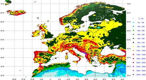
The validation of the first analysis data set revealed two distinct problems with the observations. On one hand, we identified gross errors very likely related to mistakes in the report transmission. For example, one station has sent for several consecutive days reports with amounts greater than 400 mm/day, or another even 900 mm/day. Certainly, these errors are readily managed by the analysis system when the automatic quality controls are activated. On the other hand, a more difficult problem to solve is shown in Fig. 13. Indeed, it was found that one or more stations (which are nearby each another) geographically located in a moist region as those in Latvia (Baltic area) send reports of 0 mm/day for several days or months, sometimes the reports having small gaps with reliable data. Under such circumstances, the analysis system will not be able to deal with such errors, particularly when the background also provides small precipitation amounts, unless some specific or additional criteria in the quality control and the data selection are used, or an elaborated external pre-processing treatment of the observations is performed. Figure 13 illustrates that in Latvia, systematic errors in the observations may produce analyses which do not reflect at all the climate of the region. While the surrounding countries exhibit precipitation amounts around 750 mm/year (for the year 2010), in the eastern Latvia values are less than 100 mm/year, as little as in the North-east Africa. Furthermore, in the data sparse regions or when the observations are not available as in the western Balkans (Albania, Montenegro and southern Croatia), patterns of large precipitation amounts (greater than 3000 mm/year) may occur. Consequently, the analyses are either identical or very close to the background field. As the precipitation field is discontinuous by its nature and includes interactions across multiple spatial and temporal scales, the absence of measurements in some areas will have a greater negative impact on the accuracy of the precipitation analysis than, for example, on the 2-m temperature which is a continuous field. In addition, the spatially inhomogeneous distribution of the gauge network has an influence on the quality of the precipitation analysis which in data sparse areas will reflect the one of the background and will be higher in data dense regions.

Fig. 13 Map of annual precipitation amount from 24-h precipitation analyses for the year 2010. Units mm/year.

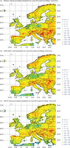
Figure 14 shows a comparison of the monthly 24-h accumulated precipitation fields for June 2010, for Mescan at 5.5 km, ERA-Interim at 25 km and GPCC at 50 km grid spacing, respectively, with the purpose of qualitatively assessing the added value of the Mescan analyses. Whereas gauge data are used to produce both GPCC (right panel) and Mescan products, the ERA-Interim (middle panel) is a forecast model field that is produced without assimilation of precipitation data. However, to produce Mescan analyses, additional gauge data from the French climatic network (non-GTS data) have been used, whereas for the GPCC products the data have come only from the GTS. Thus, a comparison of the precipitation fields over France shows that the patterns in the left panel exhibit higher, realistic amplitudes in the south-eastern and central regions than in the other panels. Furthermore, the background fields used in Mescan analyses provide a valuable information in data sparse areas such as the northern Spain where a narrow precipitation band of higher magnitude than in the middle panel can be noticed. In the right panel, there is a pattern of similar shape but of lower magnitude. At the same time, the high-resolution gridded analyses provide small-scale structures not only over mountainous regions and along the sea coasts but over flat regions as well (e.g. The Netherlands, Germany, south of the Great Britain).

Fig. 14 Maps of the monthly 24-h accumulated precipitation for June 2010 for Mescan (left panel) at 5.5 km, ERA-Interim at 25 km (middle panel) and GPCC (right panel) at 50 km grid spacing, respectively. Units mm/month.

4. Summary and conclusions

The purpose of this article was to describe and assess the performance of the Mescan precipitation system. While the Mescan system may be considered validated through the results shown in this article, the studies performed during the EURO4M project enable to tackle the issues related to the high-resolution precipitation analyses. To this aim, precipitation analyses have been performed, respectively, at 5.5 and 2.5 km grid spacing using as background fields the downscaled and native forecasts. The validation of Mescan analyses at 5.5 km grid-mesh has been done over France through the direct and indirect approaches, and the accuracy has been evaluated employing different metrics. The results have shown that in terms of categorical scores (HSS, FBI), the quality of the analyses is improved compared to the quality of the background which is a desired feature of an analysis system. In addition, the Mescan system can produce analyses that over French territory have almost the same quality as the well-validated SAFRAN analysis system (Quintana-Seguí et al., 2008).

An indirect validation has demonstrated that the 24-h precipitation analyses produced by Mescan could be used for hydrological applications. Nevertheless, further work is needed to improve the precipitation analysis, particularly in the mountainous area, and to mitigate the errors affecting the snowpack evolution. To better understand the origin of the underestimation of the river discharges for the Rhône River forced by Mescan compared to SAFRAN, further studies may concentrate on the evolution of snowpack characteristics as a function of weather conditions at the observation location.

The evaluation performed at 2.5 km grid spacing have shown that the downscaling procedure decreases the spatial variability of the forecast precipitation field. Ingesting the available observations from the SYNOP and climatic networks, the analysis system neither tends to modify the spatial variability of the native forecasts nor increases the variance of the downscaled ones. Further work should demonstrate that, by using appropriate metrics, there is an added value when using background from a very high-resolution forecast model. Such studies have not been undertaken in the current project. The spectral analysis has shown, however, the positive impact on the analyses when using high-resolution native forecasts as background fields, whereas the categorical scores have indicated a degradation of the quality of the analyses in term of HSS.

Potential improvements to the analysis scheme could also be identified by performing the analysis in the log space, testing anisotropic background error correlation functions dependent on orography or from a more appropriate selection of the observations used in the linear system such as to account for the difference of altitude between the model orography and the gauge height. The results also indicate that a bias correction procedure to improve the quality of the analyses (carried out with or without downscaled backgrounds) is needed.

6. Appendix A. Acronyms

Table

4D-Var	Four-dimensional variational data assimilation
ALADIN	Aire Limitée Adaptation Dynamique Développement International
ANTILOPE	ANalyse par spaTIaLisation hOraire des PrEcipitations
AROME	Application of Research to Operations at Mesoscale
ARPEGE	Action de Recherche Petite Echelle Grande Echellele
ECA&D	European Climate Assessment and Dataset
ECMWF	The European Centre for Medium-Range Weather Forecasts
EUMETNET	A group of European National Meteorological Services
EURO4M	European Reanalysis and Observations for Monitoring
FG5.5	First Guess at 5.5 km grid
FBI	Frequency Bias Index
GPCC	Global Precipitation Climatology Centre
GTS	Global Telecommunication System
HIRLAM	High Resolution Local Area Modelling
HSS	Heidke Skill Score
ISBA	Interaction Sol–Biosphère–Atmosphére
JMA	Japan Meteorological Agency
MODCOU	MODélisation COUplée
NCEP	National Centers for Environmental Prediction
NCAR	National Center for Atmospheric Research
NMC	National Meteorological Center now called NCEP
OPERA	Operational Programme for the Exchange of Weather Radar Information
SAFRAN	Système d'Analyse Fournissant des Renseignements Atmosphériques à la Neige
SMHI	Swedish Meteorological and Hydrological Institute
SWE	Snow Water Equivalent

5. Acknowledgements

The research leading to these results has received funding from the European Union, Seventh Framework Programme (FP7/2007-2013) under grant agreement no 242093. We gratefully acknowledge Jean-François Mahfouf for fruitful discussions, for carefully reading the early version of the manuscript and for his relevant suggestions. Also, we are grateful to Françoise Taillefer for useful discussions. We thank Per Dahlgren (SMHI) for providing HIRLAM analyses at 22 km grid, Per Undén and Ulf Andrae for assistance and constant support. We thank Albert Klein Tank (KNMI) and ECA&D team for providing readily access to the European precipitation observation data set. We also acknowledge Eric Martin and Yves Durand for fruitful discussions regarding SAFRAN system. The authors acknowledge the constructive and helpful comments of the two anonymous reviewers which helped to improve the quality of the revised version of the article.

Notes

¹Information about the EURO4M project financed by the European Union and the availability of data sets can be found at www.euro4m.eu

²For more information visit http://www.eca.knmi.nl

³See www.gpcc.dwd.de

References

- Amodei M. , Stein J . Deterministic and fuzzy verification methods for a hierarchy of numerical models. Meteorol. Appl. 2009; 16: 191–203.
- Bhargava M. , Danard M . Application of optimum interpolation to the analysis of precipitation in complex terrain. J. Appl. Meteorol. 1994; 33: 508–518.
- Courtier P. , Freydier C. , Geleyn J.-F. , Rabier F. , Rochas M . The ARPEGE project at Météo-France. Proceedings of the ECMWF Workshop on Numerical Methods in Atmospheric Models. 1991; Reading, UK, ECMWF. 193–231.
- Daley R . Atmospheric Data Analysis. 1991; Cambridge University Press, Cambridge, UK.
- Dee D. P. , Uppala S. M. , Simmons A. J. , Berrisford P. , Poli P. , co-authors . The ERA-Interim reanalysis: configuration and performance of the data assimilation system. Q. J. Roy. Meteorol. Soc. 2011; 137: 553–597.
- Denis B. , Côté J. , Laprise R . Spectral decomposition of two-dimensional atmospheric fields on limited-area domains using the discrete cosine transform (DCT). Mon. Weather. Rev. 2002; 130: 1812–1829.
- Desroziers G. , Berre L. , Chapnik B. , Poli P . Diagnosis of observation, background, and analysis-error statistics in observation space. Q. J. Roy. Meteorol. Soc. 2005; 131: 3385–3396.
- Durand Y. , Brun E. , Mérindol L. , Guyomarc'h G. , Lesaffre B. , co-authors . A meteorological estimation of relevant parameters for snow models. Ann. Glaciol. 1993; 18: 65–71.
- Durand Y. , Giraud G. , Brun E. , Mérindol L. , Martin E . A computer-based system simulating snowpack structures as a tool for regional avalanche forecasting. J. Glaciol. 1999; 45: 469–484.
- Ebert E . Fuzzy verification of high-resolution gridded forecasts: a review and proposed framework. Meteorol. Appl. 2008; 15: 51–64.
- Fortin V. Analyse de précipitation CaPA: Proposition d'installation d'une passe parallèle. Séminaire Recherche en Prévision Numérique [Precipitation Analysis CaPA: Recommendation to install a parallel suite. Workshop Research in Numerical Weather Prediction]. 2007. Dorval, QC, Environment Canada, 65 pp. Online at: http://collaboration.cmc.ec.gc.ca/science/rpn/SEM/dossiers/2007/seminaires/2007-10-26/Fortin2007RPN_CaPA_final.pdf.
- Fortin V. , Roy G. , Dobaldson N. , Mahidjiba A . Assimilation of radar quantitative precipitation estimation in the Canadian Precipitation Analysis (CaPA). J. Hydrol. 2015; 531(Part 2): 296–307.
- Fowler H. J. , Blenkinsop S. , Tebaldi C . Review linking climate change modelling to impacts studies: recent advances in downscaling techniques for hydrological modelling. Int. J. Climatol. 2007; 27: 1547–1578.
- Gelman A. , Carlin J. B. , Stern H. S. , Rubin D. B . Bayesian Data Analysis. Texts in Statistical Science. 1995; Chapman and Hall, London.
- Ghelli A. , Lalaurette F . Verifying precipitation forecasts using upscaled observations. ECMWF Newslett. 2000; 87: 9–17.
- Golaz-Cavazzi C. , Etchevers P. , Habets F. , Ledoux E. , Noilhan J . Comparison of two hydrological simulations of the Rhône basin. Phys. Chem. Earth B. 2001; 26(5–6): 461–466.
- Habets F., Boone A., Champeaux J.-L., Etchevers P., Franchisteguy L., co-authors. The Safran-Isba-Modcou (SIM) hydrometorological model applied over France. J. Geophys. Res. 2008; 113 D06113. DOI: http://dx.doi.org/10.1029/2007JD008548.
- Häggmark L. , Ivarsson K.-I. , Gollvik S. , Olofsson P.-O . Mesan, an operational mesoscale analysis system. Tellus A. 2000; 52: 2–20.
- Horányi A. , Ihász I. , Radnóti G . ARPEGE-ALADIN: a numerical weather prediction model for Central-Europe with the participation of the Hungarian Meteorological Service. Idöjárás. 1996; 100: 277–301.
- Ingleby B . Global assimilation of air temperature, humidity, wind and pressure from surface stations. Q. J. Roy. Meteorol. Soc. 2015; 141: 504–507.
- Jolliffe I. T. , Stephenson D. B . Forecast Verification: A Practitioner's Guide in Atmospheric Science. 2003; Chichester, UK: John Wiley and Sons. 240.
- Kalnay E . Atmospheric Modeling, Data Assimilation and Predictability. 2002; Cambridge University Press, Cambridge, UK.
- Kalnay E. , Kanamitsu M. , Kistler R. , Collins W. , Deaven D. , Gandin L. , co-authors . The NCEP/NCAR 40-Year reanalysis project. Bull. Am. Meteorol. Soc. 1996; 77: 437–471.
- Kistler R. , Kalnay E. , Collins W. , Saha S. , White G. , Wollen J. , co-authors . The NCEP-NCAR 50-Year reanalysis: monthly means CD-ROM and documentation. Bull. Am. Meteorol. Soc. 2001; 82: 247–267.
- Laurantin O . ANTILOPE: Hourly rainfall analysis merging radar and rain gauge data. Proceedings of the International Symposium on Weather Radar and Hydrology, Grenoble. 2008; France, 10–12 March 2008. 2–8.
- Ledoux E. , Girard G. , de Marsily G. , Deschenes J . Kluwer Academic Publishers . Spatially distributed modelling: conceptual approach, coupling surface water and ground water. Unsaturated Flow Hydrologic Modelling – Theory and Practice. 1989; , Vol. 275. Kluwer Academic, Norwell, MA, NATO ASI Series C. 435–454.
- Lespinas F. , Fortin V. , Roy G. , Rasmussen P. , Stadnyk T . Performance evaluation of the Canadian Precipitation Analysis (CaPA). J. Hyrometeorol. 2015; 16: 2045–2064.
- Lopez P . Direct 4D-Var assimilation of NCEP Stage IV radar and gauge precipitation data at ECMWF. Mon. Weather Rev. 2011; 139: 2098–2116.
- Lorenc A. C . A global three-dimensional multivariate statistical interpolation scheme. Mon. Weather Rev. 1981; 109: 701–721.
- Mahfouf J.-F. , Brasnett B. , Gagnon S . A Canadian precipitation analysis (CaPA) project: description and preliminary results. Atmos. Ocean. 2007; 45: 1–16.
- Noilhan J. , Mahfouf J.-F . The ISBA land surface parameterization scheme. Global Planet. Change. 1996; 13: 145–159.
- Onogi K. , Koide H. , Sakamoto M. , Kobayashi S. , Tsutsui J. , Hatsushika H , co-authors . JRA-25: Japanese 25-year re-analysis project progress and status. Q. J. Roy. Meteorol. Soc. 2005; 131: 3259–3268.
- Parrish D. , Derber J . The National Meteorological Center's spectral statistical interpolation analysis system. Mon. Weather Rev. 1992; 120: 1747–1763.
- Quintana-Seguí P. , Le Moigne P. , Durand Y. , Martin E. , Habets F , co-authors . Analysis of near-surface atmospheric variables: validation of the SAFRAN analysis over France. J. Appl. Meteorol. Climatol. 2008; 47: 92–107.
- Ricard D. , Lac C. , Riette S. , Legrand R. , Mary A . Kinetic energy spectra characteristics of two convection-permitting limited-area models AROME and Meso-NH. Q. J. Roy. Meteorol. Soc. 2013; 139: 1327–1341.
- Rousset F., Habets F., Gomez E., Le Moigne P., Morel S., co-authors. Hydrometeorological modeling of the Seine basin using the SAFRAN-ISBA-MODCOU system. J. Geophys. Res. 2004; 109: 1–20. DOI: http://dx.doi.org/10.1029/2003JD004403.
- Seity Y. , Brousseau P. , Malardel S. , Hello G. , Bénard P , co-authors . The AROME-France convective-scale operational model. Mon. Weather. Rev. 2011; 139: 976–991.
- Soci C., Bazile E., Besson F., Landelius T., Mahfouf J.-F., co-authors. D2.6 Report describing the new system in D2.5 EURO4M report, 26 pp. 2013. Online at: http://www.euro4m.eu/downloads/D2.6_Report_describing_the_new_system_in_D2.5.pdf.
- Talagrand O . Assimilation of observations, an introduction. J. Meteorol. Soc. Jpn. 1997; 75: 191–209.
- Uppala S. M. , Kållberg P. W. , Simmons A. J. , Andrae U. , Da Costa Bechtold V. , Fiorino M. , co-authors . The ERA-40 re-analysis. Q. J. Roy. Meteorol. Soc. 2005; 131: 2961–3012.
- Wilks D. S . Statistical Methods in the Atmospheric Sciences. 2nd ed . 2006; Academic Press, San Diego, CA.
- World Meteorological Organization. WMO-8: Guide to Meteorological Instruments and Methods of Observation. 2012; WMO, Geneva, Switzerland. updated 2010 ed.