Significance of changes in medium-range forecast scores

Abstract

The impact of developments in weather forecasting is measured using forecast verification, but many developments, though useful, have impacts of less than 0.5 % on medium-range forecast scores. Chaotic variability in the quality of individual forecasts is so large that it can be hard to achieve statistical significance when comparing these ‘smaller’ developments to a control. For example, with 60 separate forecasts and requiring a 95 % confidence level, a change in quality of the day-5 forecast needs to be larger than 1 % to be statistically significant using a Student's t-test. The first aim of this study is simply to illustrate the importance of significance testing in forecast verification, and to point out the surprisingly large sample sizes that are required to attain significance. The second aim is to see how reliable are current approaches to significance testing, following suspicion that apparently significant results may actually have been generated by chaotic variability. An independent realisation of the null hypothesis can be created using a forecast experiment containing a purely numerical perturbation, and comparing it to a control. With 1885 paired differences from about 2.5 yr of testing, an alternative significance test can be constructed that makes no statistical assumptions about the data. This is used to experimentally test the validity of the normal statistical framework for forecast scores, and it shows that the naive application of Student's t-test does generate too many false positives (i.e. false rejections of the null hypothesis). A known issue is temporal autocorrelation in forecast scores, which can be corrected by an inflation in the size of confidence range, but typical inflation factors, such as those based on an AR(1) model, are not big enough and they are affected by sampling uncertainty. Further, the importance of statistical multiplicity has not been appreciated, and this becomes particularly dangerous when many experiments are compared together. For example, across three forecast experiments, there could be roughly a 1 in 2 chance of getting a false positive. However, if correctly adjusted for autocorrelation, and when the effects of multiplicity are properly treated using a Šidák correction, the t-test is a reliable way of finding the significance of changes in forecast scores.

• statistical significance
• forecast verification
• Student's t
• temporal autocorrelation
• paired differences
• multiple comparisons

1. Introduction

Forecast verification is central to the ongoing development of weather prediction. Every year, a Numerical Weather Prediction (NWP) centre will trial dozens of scientific developments before they are merged into an upgrade of the forecasting system. The quality of medium-range forecasts in the northern extratropics is improving by around 10–20 % per decade at centres such as the European Centre for Medium-Range Weather Forecasts (ECMWF; e.g. Simmons and Hollingsworth, 2002; Magnusson and Källén, 2013). Although some of that comes from step-changes like the introduction of variational data assimilation (e.g. Andersson et al., 1998), most of the improvement likely comes from the flow of smaller developments like model parametrisation upgrades or newly launched satellites. These changes often have less than 0.5 % impact, which is hard to detect with forecast verification (note also that improvements do not necessarily add linearly, so it takes many smaller developments to achieve a 20 % improvement per decade).

The central problem is that chaotic error growth leads to large differences in skill between any two forecasts (e.g. Hodyss and Majumdar, 2007). Even when verification from hundreds of forecasts is combined, these chaotic differences are large enough to cause appreciable differences in average forecast scores. As will be shown, two perturbed but otherwise identical model configurations can differ by 1 % in forecast error when computed from a sample of 60 forecasts. A real change in error of 0.5 % is undetectable in this context. To verify any scientific change at ECMWF, it is now routine to use at least 360 forecasts. One aim of this study is to investigate the size of sample required to reliably test a development in a high-quality forecasting system. A broader hope is to encourage better practice in evaluating scientific developments in forecasting which are still sometimes documented without considering the possible impact of chaotic variability on the results.

Statistical significance testing is becoming more widespread in meteorology (Ebert et al., 2013) and the statistical background is given by Jolliffe (2007) while textbooks cover all the fundamentals (von Storch and Zwiers, 1999; Wilks, 2006). However, although forecasting centres tend to rely on a Student's t significance test applied to paired differences in forecast errors, this is not much examined in the literature. The textbook on forecast verification by Jolliffe and Stephenson (2012) devotes only a few pages to the subject of significance. Rather, the focus has been on the development of more sophisticated verification techniques that do not always see widespread use (Casati et al., 2008). At ECMWF, the paired difference approach was set in place by Mike Fisher (1998), though only in an internal publication. It is hoped the current work will help to address the documentation deficit, so it will summarise the basics in Section 3.

Even when significance testing is applied, scientists question its reliability: some think the significance tests are over-cautious but others wonder if some unusual statistical property of forecast scores might cause significance to be overestimated. This author's suspicion was that too many results were simply the result of chaotic variability. In a recent example, a set of 360-sample experiments needed to be repeated after the discovery of a compiler bug. The code generated by the improved compiler was not bit-reproducible with before, leading to chaotic divergence (e.g. Lorenz, 1963) between the original and the new experiment. Statistically significant impact at day 7 moved from the Northern Hemisphere (NH) to the Southern Hemisphere (SH), suggesting at minimum that no significance was associated with the hemisphere in which the impact appeared (Geer et al., 2014, discussion of their Fig. 20). Although the compiler bug might have affected forecast quality, it is most likely that the tests of statistical significance were too generous. Hence a second aim is to explore the validity of the current approach, which has not been fully established. Fisher (1998) showed that temporal autocorrelation was important and introduced a correction for the t-test. The current study will also investigate the issue of multiple comparison (e.g. Benjamini and Hochberg, 1995) as a possible explanation. However, we should also question the assumptions of Gaussianity, randomness and independence built into the Student's t-test.

At the heart of significance testing is the null hypothesis. In the case of forecast verification, we would like to test the null hypothesis that a perturbation to the forecasting system gives no improvement or deterioration in forecast error, on average. The null hypothesis built into the Student's t-test is just a model of this, and it assumes that forecast error differences are independent and distributed randomly with a Gaussian distribution. However, a forecasting system is not random but chaotic, and its errors are not independent from one forecast to the next; there is no guarantee that its statistics will be modelled correctly in the t-test. The example of the compiler upgrade that affected the experimental results of Geer et al. (2014) is a more practical model for the null hypothesis, and it motivates the central idea of the current work: that it is totally feasible, if expensive, to explicitly compute a null population using perturbed but otherwise identical experiments. The results of this study will be based on a sample of 1885 pairs of forecasts covering 2.5 yr of experimentation. This independent realisation of the null population can be used to experimentally test the assumptions that are being made in the classical approach. It can also be used to create an entirely non-parametric significance test, that is, one that makes no assumptions on the distributions of forecast scores. These are the new tools to be used in this study.

This study will be restricted to medium range (day 3 to day 10) extratropical forecast scores of which the quintessential example is the root-mean-square (RMS) error in 500-hPa geopotential height (e.g. Lorenz, 1982). As will be illustrated in the next section, these scores are mainly sensitive to large-scale errors in the location of the low- and high-pressure features of extratropical Rossby waves. The quality of modern synoptic analyses is very good, but over a 10-d forecast the errors grow rapidly. Since the errors that are being measured are large compared to the errors in the reference (i.e. the analysis) and little affected by small-scale features, these traditional extratropical scores are robust measures of synoptic-scale error. For example, the standard deviation and the RMS error are almost identical, demonstrating there is little systematic error, and the exact scale of the verification grid is unimportant (unpublished work by the author). To limit the scope of the problem, this study will explicitly exclude situations where errors in the reference are closer in size to those of the forecasts being verified, that is, verification of the stratosphere, the tropics, and the first few days of the forecast. The difficulties of forecast verification in these situations will hopefully be the subject of further investigation, and of course such problems have motivated much work in the past (e.g. Murphy, 1988; Thorpe et al., 2013).

The error of synoptic forecasts is not the only measure of forecast skill: many users of forecasts are more concerned with variables like near-surface temperature, cloud and rain. However, it is still important to check that upgrades do not cause harm to the large-scale forecast. Problems can come through scientific oversights, unforeseen interactions or simply from coding errors. The intention is not to exclude other valuable approaches in forecast testing and verification, but forecast quality at most ranges and scales is dependent on the synoptic forecast, so these basic scores will always be important.

2. Experiments

This study is based on full-cycling data assimilation and forecast experiments covering 1 January 2011 to 31 July 2013. 1885 forecasts are available, initialised twice-daily from analyses at 00Z and 12Z. Experiments use ECMWF cycle 38r2 which was operational during 2013 and has 137 vertical levels. A horizontal grid T511 equivalent to about 40-km resolution has been chosen, lower than the operational resolution but far cheaper to run, and only a little less skilful at the medium range. Forecasts are verified at ranges from 12 h through to 10 d, against the experiment's own analysis, so some forecasts at the end of the period cannot be verified. The precise number of forecasts verified varies from 1885 to 1866 for the 12-h to 10-d forecast.

Table 1 summarises the three experiments used in this study. The perturbation experiment will be explained in Section 4. As well as the control and perturbation experiment, routine scientific testing is illustrated by removing one Advanced Microwave Sounding Unit (AMSU-A, on the satellite Metop-A; Robel, 2009) from the global observing system. AMSU-As measure temperature in broad vertical layers across the vertical extent of the atmosphere and AMSU-As on seven satellites are the most influential group of observations for medium-range forecasting (e.g. Radnoti et al., 2010). But the typical decision being made at an operational centre is not whether this type of observation should exist at all, which would cause a large impact on scores, but whether to add one extra satellite. Borrowing an economics concept, what matters is marginal impact. As will be shown, going from six to seven AMSU-As gives a 0.5 % improvement in forecast scores at day 5, which would be a useful contribution to the (roughly) 2 % per year improvement in scores from all developments in data assimilation, modelling and the observing system.

Table 1. Experiments used in this study

Name	Description
Control	ECMWF operational configuration (cycle 38r2) with all observations but with T511 horizontal resolution.
Perturbation	Scientifically identical to the control, but with a technical modification that results in numerical differences in some operators in the data assimilation, compared to the control. See Section 4.
AMSU-A denial	The AMSU-A on Metop-A has been removed from the observing system.

3. Basics

Forecasts are generated from a set of assimilation experiments and verified against the best estimate of the true atmospheric state, which is usually an analysis. For a field of m model grid-points j, forecasts f _j are compared to analyses a _j valid at the same time. The RMS error r can be computed as:1

Weights w _j sum to 1 and are proportional to the area of the grid-box. Statistics are usually computed over set regions of the globe, here the Northern Hemisphere and Southern Hemisphere (excluding the tropics) defined as 20°N–90°N and 20°S–90°S. Atmospheric fields are interpolated to a regular latitude–longitude grid, in this case 2.5°, before computing the RMS error. This study concentrates on RMS scores which are the simplest to compute and most popular; other choices such as anomaly correlation or standard deviation can be used, but when considering midlatitude synoptic scores the results are very similar – this will be justified later.

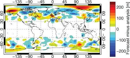
Figure 1 shows forecast minus analysed 500-hPa geopotential height on a typical day in the northern winter. These are the f _j –a _j available to eq. (11 ), though note the weighting term w _j reduces the influence of the errors at high latitudes compared to their visual prominence in this projection, particularly poleward of 75°. Errors are spatially quite smooth and contiguous across areas at least 1000 km in extent. It is clear that day 5 forecast errors in 500-hPa height measure inaccuracies in the large-scale synoptic forecast in the midlatitudes. Small-scale errors have little impact on the RMS and there is no need to use a higher resolution than 2.5° to compute these scores. Tropical regions exhibit little variability in geopotential, hence the relative lack of errors there. The situation is similar through the medium range but in the short-range, errors are generally on scales of 500 km or less (not shown). Interestingly, day-5 wind errors exhibit smaller scales (e.g. 500 km, not shown) but as will be seen, regional wind scores are highly correlated with geopotential height errors.

Fig. 1 Day-5 forecast minus analysed geopotential height at 500 hPa in the control experiment, at 00Z on 31 January 2012.

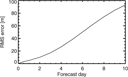
The RMS error as a function of lead-time (Fig. 2) illustrates the rapid baroclinic error growth in midlatitudes. As mentioned, the experiment's ‘own analysis’ has been chosen as the verification reference. Where the experiments are comparable in skill and close in quality to the best available, the own analysis is a reasonable choice of reference because it avoids various possibilities of biasing the comparison in the early forecast range (e.g. Geer et al., 2010; Bowler et al., 2015). However, the forecast error at the initial time is by definition zero, which is unsatisfactory and incorrect. Nevertheless, issues of short-range verification are not the subject of the current study. All results and figures in this study have also been repeated using the ECMWF operational forecast as the reference. However, such a change in the reference has negligible effect on this study. Appendix A gives further details.

Fig. 2 RMS error of NH geopotential height at 500 hPa in the control experiment, as a function of forecast lead time, for the control experiment, aggregated over 1 January 2011 to 31 July 2013.

A noteworthy aspect of the typical statistical framework is that each forecast is verified individually, and then the scores are averaged arithmetically. Figure 2 shows the mean of the RMS over the n forecasts (1875 at day 5 in this example) with i representing each forecast:2

One reason to treat the r _i as separate samples is to provide a population to which the Student's t-test can be applied. An alternative approach would be to compute the RMS [eq. (11 )] across all grid-points and forecast times simultaneously, but that would make it more difficult to devise a hypothesis test, and the results would likely be dominated by large winter errors (in the same way that an RMS computed globally over Fig. 1 would be dominated by errors of the NH winter.)

Figure 3a shows the evolution of day-5 RMS error of Northern Hemisphere (NH, 20°N–90°N) geopotential height in the control run. The most obvious feature in RMS error is the seasonal cycle, with errors reaching 65 m winter and sometimes reducing to 20 m in summer. This reflects the larger amplitude of Rossby waves in winter. It is clear that forecast scores tend to be correlated from one day to the next, with periods of smaller or larger errors persisting for at least a week, reflecting the amplitude and predictability of the evolving weather patterns. Autocorrelation between RMS scores of successive forecasts (every 12 h) and every second forecast (every 24 h) are 0.76 and 0.6, respectively. For this reason, scores are highly correlated between different experiments, as illustrated in panel b. The scientific components in these experiments (e.g. forecast model, the vast majority of observations) are mostly identical and that must also contribute to the correlation between them. Still, the denial of an AMSU-A is a fairly important scientific perturbation of the system but it seems to make little difference to the forecast scores. There is little hope of applying a t-test to these results: control and experiment are highly correlated, and (not shown) their PDFs are not Gaussian, having a fat tail in the direction of higher errors, that is, towards forecast ‘busts’. This reflects the non-linear, chaotic nature of synoptic forecasts.

Fig. 3 Time series of (a) RMS error of 500-hPa NH geopotential height at day 5 in the control experiment (black), verified against an own-analysis reference. (b) As (a), but covering a shorter period of time and including scores from the AMSU-A experiment (red). (c) Experiment minus control over the full time period.

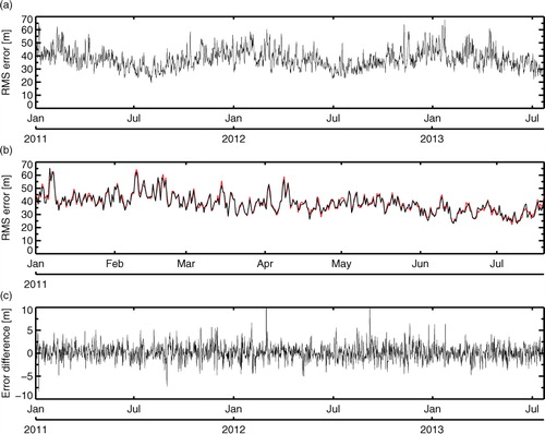
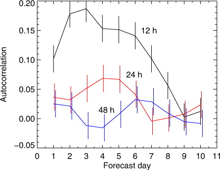
The solution (Fisher, 1998; von Storch and Zwiers, 1999; Wilks, 2006) is to look at the paired differences, that is, the time series of:3 This is shown in Fig. 3c; seasonal variability and forecast-to-forecast correlation appear to have been removed. Figure 4 shows the time-autocorrelations at various forecast validity times. At day-5 these are 0.15 for base times separated by 12 h, 0.07 for separations of 24 h and essentially zero for any longer period. As shown by Fisher and later in this study, to get the statistical testing exactly right, it is important to deal with the autocorrelation. However, for now we will assume that taking paired differences has created a statistical population that has sufficiently little autocorrelation that a normal t-test can be used to test for statistical significance.

Fig. 4 Time autocorrelation of paired differences (AMSU-A Denial minus control) in RMS error of NH geopotential height at 500 hPa, as a function of forecast lead-time. Autocorrelations are shown for forecasts separated by 12 h (black), 24 h (red) and 48 h (blue). This pattern is representative of all tropospheric levels in the NH and for other choices of forecast score, such as anomaly correlation, or the RMS error in temperature or vector wind. However, autocorrelation becomes very significant in the stratosphere, where systematic errors dominate RMS forecast scores, and it is slightly larger in the SH. Error bars have been estimated with a Monte-Carlo approach: they are represented by the standard deviation of a large number of lag-1 autocorrelations estimated from samples of 1885 normally distributed random numbers.

We want to know how the forecast scores of the experiment differ from the control and the usual way is to compute the mean of the paired differences across the n forecasts:4

In this example, , so eliminating one AMSU-A appears to degrade the scores, that is, it makes RMS errors slightly larger. However, this is small in comparison to the standard deviation s of the paired differences, which is 1.76 m in this example. The question is whether this 0.18 m increase in error is statistically significant.

The usual null hypothesis in forecast verification is that forecast-to-forecast variability in d _i is purely random and centred on zero. The null hypothesis gives rise to a null population, which is an infinite set of random differences between forecast scores d _i . As explained earlier, we are attempting to represent a different and more precise null hypothesis: that there is no mean difference in scores and that any sampling error in mean scores computed from finite samples comes from the chaotic variability of paired differences in forecast quality, which may or may not be independent, random or Gaussian.

Given the mean and standard deviation s of the paired differences, a test statistic z can be computed (e.g. Wilks, 2006):5

If the null hypothesis is true, z can be shown to follow a t-distribution (Student, 1908) which varies according to the population size n but for larger n it tends towards a standard Gaussian (i.e. one with unit standard deviation and zero mean). In the paired difference test, the mean of the null population µ ₀ is zero, so it will not be written explicitly from now on. k is an inflation factor to account for autocorrelation or other effects that might affect the results. This will be useful later but for the moment we assume no inflation so k=1. The t-test recognises that a mean computed from a finite sample is an uncertain estimate of the true mean of the population. z is essentially the ratio of the mean of the population (e.g. ) to an estimate of the sampling error in that mean, that is, . For smaller n (e.g. less than 50), the t-distribution is broadened compared to a standard Gaussian because of the uncertainty in s as an estimate of the population standard deviation.

By comparing the test statistic z to the t-distribution, we can determine the consistency of the result with the null hypothesis. For large sample sizes, 95 % of the t-distribution falls within ±1.96. In our example, z=4.52, which is far outside the usual range of the t-distribution. Even though eliminating one AMSU-A increases forecast errors by only 0.18 m, this is still a highly significant result in the context of 2.5 yr of experimentation. If the null hypothesis were true, the probability of this occurring, p, would only be 2×10⁻⁵. It is usual in forecast verification to declare as statistically significant any result which has less than p=0.05 chance of being consistent with the null hypothesis. Although many scientific fields refer to this p value, in forecast verification we typically call this a 95 % (i.e. (1 − p)×100 %) confidence level. It is worth noting that normally a ‘two-tailed’ test is applied, that is, that we are interested both in situations where the forecast scores get worse or better.

The difference in forecast scores is usually presented against forecast lead-time (Fig. 5) by normalising with the forecast score of the control, that is, . Statistical significance testing is conventionally represented using an ‘error bar’ illustrating the 95 % probability range of the t-distribution. This can be labelled ±z ₉₅ (i.e. for larger samples, ±1.96 in z-space). To convert this to a normalised difference in forecast error, we first obtain the equivalent confidence range ±d ₉₅ by substitution into eq. (55 ):6

Fig. 5 Normalised change in RMS error of NH geopotential height at 500 hPa (AMSU-A denial minus control) as a function of forecast lead-time, aggregated over 1866–1885 forecasts between 1 January 2011 and 31 July 2013. Vertical bars (which should not be confused with regular error bars) give the 95 % confidence range.

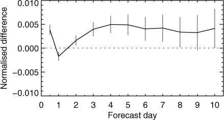
(note how k gives a way of inflating the confidence range if needed, but it equals 1 for the moment). The range ±d ₉₅ can then be normalised by and centred on the forecast score to produce the range plotted in Fig. 5.

To be strictly correct, the confidence range should be centred on the zero line (this style of plotting will be demonstrated later) and not on the forecast score. Centring on the forecast score makes it easy to conflate the confidence range with a typical error bar, which is something very different, that is, the standard error of an estimate. However, the score-centred confidence range is widely used, maybe because when several forecast experiments are placed on the same figure, it becomes possible to judge (in an approximate way) the statistical significance of differences between the experiments as well as between those experiments and the control.

Figure 5 shows the forecast impact of removing one AMSU-A from the global observing system. Though impossible to identify in Fig. 3, this has a statistically significant impact of around 0.5 % increase in forecast error from day 3 through to day 8. But the random variability (s) of forecasts beyond day 8 is so large that even with our very large sample it is impossible to confirm whether eliminating one of seven AMSU-As affects the scores. There is also some strange behaviour up to day 2, which relates to problems in short-range verification including systematic error, but is not the subject of this study. In most routine verification, it is impossible to achieve a sample size remotely as large as used in this example. For verification over a couple of months with n=120, the confidence range would be times larger, as inferred from eq. (66 ). There would be no statistical significance in any of the results in Fig. 5. The issues of interest in this study are first, to see how far these confidence ranges can be trusted and second, to demonstrate the size of sample required to generate significant results.

4. The null distribution

As explained in the introduction, it is possible to generate a real null population by making an ‘upgrade’ to the forecasting system that has no scientific impact. This will be called the ‘perturbation experiment’ and it can be achieved by making a purely technical change that alters the numerical reproducibility of the forecasting system without altering any of the science. Appendix B gives the technical details of how this is done. Normal chaotic error growth causes a rapid divergence between any two assimilation experiments into which even the slightest numerical perturbation is introduced – just as seen by Lorenz (1963). Although the observations are the same in both experiments and they keep the analyses on a similar path, the analyses can still take a range of plausible solutions within the range of error of the observations and the model first guess. The forecasts made from those analyses will also vary. The control and the perturbation experiment could be seen as a crude two-member ensemble of data assimilations (EDA). An EDA is used operationally at ECMWF to estimate flow-dependent background errors for the main analysis, and the additional ingredients are broadly just more members, plus perturbations to the observations and to a few model parameters (Isaksen et al., 2010; Bonavita et al., 2015). Due to the additional perturbations applied, the spread of a true EDA is likely to be larger than that between the perturbation and control experiment, so it would not be an appropriate representation of the null distribution we are interested in here.

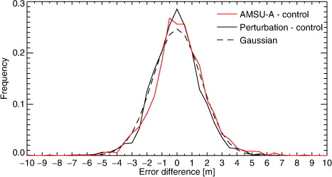
Figure 6 shows histograms of the paired differences between the AMSU-A experiment and the control (as shown in Fig. 3c) and between the perturbation experiment and the control. The histograms are both very similar, and close to a Gaussian in shape. They are not the smooth curves we might hope for, because even with 1876 samples there are sampling errors in the PDF, compared to one generated from an infinite population. However, the greater errors in the AMSU-A denial experiment show themselves as a general shift to the right compared to the null population. Forecast degradations of greater than 6 m occur on eight occasions in the AMSU-A denial experiment and on just one occasion in the perturbation experiment. These might be cases where the AMSU-A observations that were removed were particularly critical to forecast skill, perhaps because they observed an area associated with rapidly growing forecast errors. However, it is hard to ascribe statistical significance to that, and the main effect of removing one AMSU-A is to increase forecast errors by a small amount on average. Apart from this rightwards shift, the PDF of AMSU-A differences looks very similar to that from the perturbation experiment. Hence, most of the variability in the AMSU-A differences (e.g. Fig. 3c) must come from the same source as that in the perturbation experiment: chaotic variability in the quality of forecast scores.

Fig. 6 Histograms of paired differences in NH RMS 500-hPa geopotential height errors at day 5. A Gaussian is plotted that has the same standard deviation as the perturbation minus control population. The integral of this histogram is normalised to 1 (it is a PDF). Bins are 0.5 m in size. Each population has 1876 members.

Table 2 summarises statistical properties of the samples in Fig. 6, as well as those at other forecast times. As is indicated by the confidence ranges plotted in Fig. 5, at longer forecast ranges it is harder to be sure that the AMSU-A experiment has genuinely larger forecast errors than the perturbation experiment, because the chaotic variability of scores is so much larger. To underline this, at day 10, the AMSU-A denial and the perturbation experiment both apparently cause an increase in error, of very similar magnitude (0.38 m or 0.35 m). The standard deviations of the paired differences for the AMSU-A experiment are similar to those from the perturbation experiment, supporting the normal approach of using the standard deviation of the population under test to represent that of the null population.

Table 2. Statistical properties of the paired differences in NH RMS 500-hPa geopotential height errors at various forecast ranges

Name	Day	Mean [m]	Std. dev. [m]	Skewness	Kurtosis
AMSU-A-	3	0.07	0.55	−0.10	2.67
control	5	0.18	1.77	0.47	3.60
	7	0.26	3.90	0.21	1.92
	10	0.38	8.43	−0.06	1.27
Perturbation-	3	−0.01	0.48	−0.13	1.76
control	5	−0.04	1.62	−0.12	1.61
	7	0.12	3.63	0.14	1.10
	10	0.35	8.30	0.08	0.51

The skewness and kurtosis in Table 2 indicate minor deviations from Gaussianity, and it appears that kurtosis becomes smaller in the longer forecast ranges. Bigger samples should give more reliable results, and this can be achieved by combining populations at different forecast ranges and also from the Southern and Northern Hemisphere, noting that the shapes of the PDFs are similar at different time ranges and in the different hemispheres (not shown). However these scores must be independent, otherwise the combined PDF will be artificially broadened (see Wilks, 2006). Using correlation to estimate independence, Section 7 will show that paired differences in forecast scores are correlated to about 5 d in forecast lead-time and across most of the vertical extent of the troposphere. Having excluded the tropics, the stratosphere and the early forecast range (up to day 3 here, for safety) there are only around four independent sets of hemispheric scores available to make a bigger sample: day 4 and day 10 in the SH and NH. These sets are standardised by dividing by their standard deviation and Fig. 7 shows the results, which are very similar to Fig. 5. Both the AMSU-A and the perturbation differences have skewness and kurtosis relatively close to those expected from a true Gaussian (Table 3). However, a chi-squared test (see Wilks, 2006) would reject the hypothesis that these curves are Gaussian. It will be shown later that this level of non-Gaussianity has no real effect on the significance testing of forecast scores, presumably due to the central limit theorem.

Fig. 7 Histograms of paired differences in RMS 500-hPa geopotential height errors, standardised by dividing by the standard deviation of four sub-populations (day 4 and day 10 in both SH and NH). This gives a population of 7464 in each histogram. The dashed line is the standard Gaussian. Bin size is 0.2 and the integral of the PDF across all bins is 1.

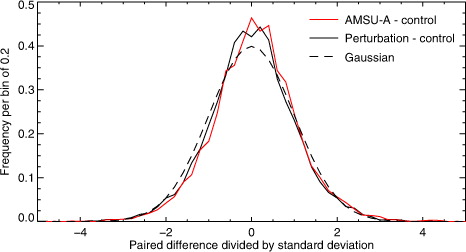
Table 3. Skewness, kurtosis and chi-squared of the populations shown in Fig. 7

Name	Skewness	Kurtosis	Chi-squared
AMSU-A- control	0.145	1.39	1045
Perturbation- control	−0.053	1.30	168.9

A Gaussian will have a skewness of 0 and kurtosis of 0 by the definitions used here. Chi-squared is computed against the Gaussian on the 47 bins between −4.6 and +4.6, and would have to be less than 60.4 to confirm Gaussianity at the 95 % confidence level.

It is worth restating the most important conclusion from this section: the differences in forecast scores between any pair of experiments show a lot of variability, but almost all of it is down to chaotic variations in the quality of forecast scores. The average changes in forecast quality resulting from a typical upgrade to an operational forecasting system are many times smaller than the standard deviation of this variability. Identifying small genuine changes in forecast scores is difficult.

5. Establishing significance in shorter experiments

So far we have examined the results from 2.5 yr of forecast verification, which is unaffordable on a routine basis. What if only 1 month of experimentation, that is, 60 forecasts, were available? There are 31 different non-overlapping, contiguous blocks of this length in the long experiments, so it is possible to compute the mean change in forecast scores for each of them. Figure 8 shows a histogram of the results from each block, at day 5 in the NH as usual. Over the complete period with 1876 forecasts, removing an AMSU-A has been seen to increase forecast errors by 0.18 m compared to a 95 % confidence range of ±0.08 m, based on Table 2 and eq. (66 ) (still assuming k=1). The 95 % confidence range for 60 forecasts would be ±0.44 m. At this confidence range, removing one AMSU-A would only have given statistically significant results in 5 of the 31 blocks. The 26 results that did not reject the null hypothesis illustrate ‘type-II’ failures of the significance test. Here, the null hypothesis is in fact false (as we have shown over the full set of 1876 forecasts) but there is insufficient statistical ‘power’ to distinguish that. There might be a temptation to reduce the size of the confidence range, for example, to 80 %, which would result in a significance threshold of ±0.29 m. However, the 60-forecast blocks from the perturbation experiment illustrate why this could be a bad idea: there are 3 of 31 blocks significant at the 95 % level and 13 of 31 significant at the 80 % level. The perturbation experiment — changing the number of parallel processors used in the ECMWF forecasting system — is not a real scientific change and should not appear as such. Rejecting the null hypothesis when it is actually true is a ‘type-I’ failure of the test. The philosophy in the rest of this work is to focus on correctly limiting type-I errors to the 95 % confidence level, assuming that type-II errors can be reduced by extending the length of the forecast testing and better designing our forecasting experiments (how to achieve this practically will be discussed later). At a broader level, the point of Fig. 8 is to illustrate how hard it is to identify, in any statistical way, the difference between small samples drawn from the perturbation and the AMSU-A experiment.

Fig. 8 The uncertainty of forecast differences computed over one month (i.e. 60 forecasts). The figure shows histograms of the mean of paired differences in NH RMS 500-hPa geopotential height errors at day 5. There are 31 different contiguous 60-forecast samples available in the 2.5-yr experimental period. Bin size is 0.1 m. The dashed line shows the t-distribution transformed into the space in which we are computing means.

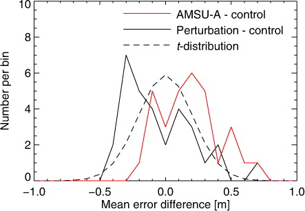
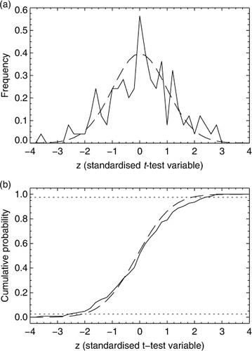
If the t-test is valid for forecast scores, then the block-means computed from the explicit null population should exactly follow a t-distribution. The number of blocks in Fig. 8 is too small to test this robustly, but more blocks can be found by looking at a combined sample of scores from the NH and SH, day-4 and day-10 as in Section 4. Taking samples of 60 contiguous and non-overlapping forecasts, there are then 124 different independent t-tests that can be performed on the explicit null population. The z-scores from each of these tests are summarised in Fig. 9a. Making allowances for what is still a small sample, they appear to be distributed according to the t-distribution. However, there are too many z-values in the tails, that is, with magnitudes greater than 2. The t-test, as it has been applied so far without accounting for autocorrelation, is too generous and gives more false positives than expected. The cumulative distribution function (CDF) of these z-scores is shown in Fig. 9b and could be used to construct a significance test free from any of the statistical assumptions needed for the Student's t approach. The 95 % confidence limits would be at about ±2.5 rather than ±2.0 in the t-test. Accounting for this using the inflation factor k in eq. (66 ), k=2.5/2.0=1.25. Assuming that this result is valid for all sample sizes, the confidence ranges presented in Fig. 5 should be increased in size by 25 %. A more rigorous examination of this result will be made in Section 6 which shows that the need for an inflated confidence range can be explained by temporal autocorrelation, as originally proposed by Fisher (1998). For now, we will concentrate on the even more important issue of the impact of chaotic variability on the scores computed from ‘smaller’ samples.

Fig. 9 The result of performing t-tests on samples from the explicitly generated null population, that is, the differences between the perturbation and control experiments: (a) PDF of z-tests generated from blocks of 60 paired forecast differences (solid) and the Student's t-distribution (dashed); (b) CDF of the same. Dotted horizontal lines indicates the 2.5 and 97.5 % quantiles, the limits of the 95 % confidence test. Based on a total of 124 independent blocks, 31 from each of the SH and NH at day 4 and day 10. Bin size is 0.25.

It is now rare to present results from forecast systems based on only 1 month of testing, so we can examine a more typical sample size of 230 forecasts, which is nearly 4 months of experimentation, and divides the 2.5 yr experiment period into eight separate non-overlapping, contiguous blocks. Also it is more typical to present normalised changes in forecast scores against forecast validity time, so the results from the eight blocks are shown in this way in Fig. 10. Two confidence ranges are included, one based on a t-test without inflation and a broader one with the 25 % inflation factor suggested by Fig. 9. For the AMSU-A minus control experiments in panel a, only four of these blocks give statistically significant results at day 3 or beyond according to the inflated t-test. Even a 230-day AMSU-A denial experiment will have too little statistical significance to give reliable conclusions: type-II error still dominates.

Fig. 10 Normalised change in NH 500-hPa height RMS forecast error: a) AMSU-A minus control; b) perturbation minus control. Separate lines are shown for eight independent blocks of 230 forecasts. Change in error is normalised by the RMS error of the control experiment. The shading indicates the 95 % confidence range estimated in the normal way (no inflation, dark grey) or with the 25 % inflation factor estimated from the explicit null population (light grey). To compute the confidence range, the standard deviation of paired differences computed from all 2.5 yr of samples in the null distribution has been used. It is centred on zero, which is more statistically correct than centring on the experimental result (the method used in Fig. 5). This approach gives less visual clutter when many experiments are presented on the same figure.

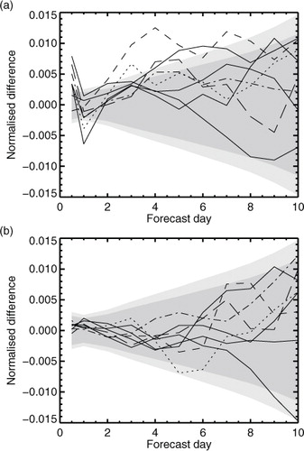
The perturbation experiment should not be mistaken for a genuine change in forecast scores, but if the t-test were done without inflation (the narrower confidence range in Fig. 10b), five of the eight perturbation experiments would show at least one instance of ‘statistically significant’ improvement. This illustrates how important it is to get the confidence range exactly right, and why narrowly significant results should be treated with caution. More generally, comparing both panels of Fig. 10, even with 230 samples, it would be hard to identify any difference in the results between many of the AMSU-A denial experiments and many of the perturbation experiments.

6. The inflation factor and temporal autocorrelation

Section 5 has shown the need for an inflation factor of around 25 % when using the t-test, using the explicitly generated null population and making no statistical assumptions. Possible statistical explanations for this are the violation of assumptions of Gaussianity, independence and randomness in the t-test. The main aim of this section is to explain the inflation factor and find how best to estimate it in practice using normal statistical tools, and finally to validate those tools against the experimentally derived null distribution.

Before coming back to the populations of real forecast scores, these issues can be investigated using Monte-Carlo simulations. The analysis performed in Fig. 9 can be repeated with distributions made from normally distributed random numbers and is shown in Fig. 11. As seen earlier (Table 2, 3 and Fig. 7) the paired differences of forecast scores have appreciable kurtosis, more outliers than might be expected, and high chi-squared values. It was found that a non-Gaussian PDF with such features could be simulated by shuffling together two distributions: a) putting 1 000 000 random numbers into a t-distribution with 8 degrees of freedom (using the t-distribution here simply as a convenient way of generating non-Gaussianity); b) to boost the tails of the PDF, 40 000 additional random numbers from a constant (rectangular) distribution between −4 and +4. This generated a population with a kurtosis of 1.3 and chi-squared of 36 399, similar to the real scores, though with the non-Gaussianity slightly exaggerated. However, the PDF and CDF of the means computed from 60-sample blocks was essentially no different from that predicted by the t-distribution (used conventionally, with 59 degrees of freedom). This is consistent with the central limit theorem: averages computed from a population are expected to be normally distributed even if the population distribution is not Gaussian itself. Hence the minor non-Gaussianity of the real forecast score differences can already be ruled out as the likely cause of the inflated error bars.

Fig. 11 As Fig. 9, but based on randomly generated populations representing a true Gaussian (dashed), an uncorrelated non-Gaussian population with a kurtosis of 1.3 (solid black, barely distinguishable from the Gaussian), a Gaussian population with 0.07 autocorrelation, representing forecasts made 24 h apart (red) or with [0.15, 0.07] autocorrelation, representing forecasts made 12 h apart (blue). Results are based on 16 666 non-overlapping blocks each containing 60 samples.

Figure 4 shows that paired forecast differences at day-5 have an autocorrelation of 0.15 across 12-h separations samples and 0.07 across 24 h forecast spacing. This autocorrelation can be simulated by convolving a normally distributed random number sequence with an appropriately chosen kernel, as described in Appendix C. Figure 11 also examines the influence of this temporal autocorrelation on the results of t-tests. This broadens the sampling distribution so that the confidence range would need to be inflated to ±2.5 in z-space. The autocorrelation problem could be reduced by only including forecasts every 24 h, rather than every 12 h. Simulations have been made for this too, showing that an inflated confidence range of perhaps ±2.1 would be required (whether spacing forecasts more widely in time is a good strategy is examined in Section 9). Overall, it looks like the temporal autocorrelation of paired differences is sufficient to explain the broadening of the t-distribution observed with real forecast scores in Fig. 9; there does not appear to be any other problem with the randomness or Gaussianity of paired differences generated from forecast experiments, even if they are generated from a chaotic rather than a random system.

As shown by Fisher (1998), and more generally by, for example, Wilks (2006), in the t-test of the paired differences in forecast scores, it is possible to account for the effect of temporal autocorrelation using autoregression (AR) models. Temporal autocorrelation increases the variance of the sampling distribution of the mean relative to the variance of the sample, which can be represented with an inflation factor k where7 and the sample mean , sample standard deviation s and sample size n have already been introduced in Section 3. The t-test, in eq. (55 ), computes the ratio of the sample mean to its estimated sampling error, so the inflation factor k describes the increase in that expected sampling error. Assuming an autoregression model fits the data, it can be used to compute the inflation factor k as a function of the population autocorrelation, as outlined in Appendix C.

Table 4 shows estimates of the inflation factor k using the autoregressive approach. The lag-1 and lag-2 autocorrelation of the day-5 NH paired AMSU-A minus control differences from Fig. 4 have been used, based on the complete population of 1866–1885 samples (autocorrelations from the perturbation-control population are not significantly different from the AMSU-A-control population). There is appreciable sampling error in the autocorrelation and this propagates into the inflation factor estimates (see Appendix C). Using the AR(1) model applied to forecast scores with 24 h spacing would give an inflation factor of k=1.07±0.02, consistent with the results of Fisher (1998). Since then, many scientists have moved to using forecasts separated by 12 h; applying the AR(1) model in this situation gives k=1.16±0.02, which is an underestimate because it does not correctly take into account the lag-2 autocorrelation. The AR(2) model gives k=1.22±0.04, consistent with the results generated from the simulated null population in Fig. 9.

Table 4. Estimates of k using autoregressive models and the autocorrelations for day-5 NH geopotential paired differences from Fig. 4, either for 12 or 24 h separation between forecasts

		Autocorrelation
Model	Forecast separation	Lag-1	Lag-2	k
AR(1)	24	0.07	N/A	1.07±0.02
AR(1)	12	0.15	N/A	1.16±0.02
AR(2)	12	0.15	0.07	1.22±0.04

A Monte-Carlo technique has been used to estimate the standard deviation of error in the k estimate (see Appendix C).

To test this conclusion more rigorously, the method of estimating k from the explicit null population has been automated. It can be applied to sample sizes other than the 60-forecast blocks used in Fig. 9 and it can be applied to the individual components (e.g. NH, SH, day-4 and day-10) as well as to combined samples. To reduce quantisation in the results, the bin size used for computing the CDF is 0.01 in the automated approach rather than 0.25 as shown in the figure. Further, assuming that the distribution should be symmetric, z ₉₅ is estimated as the average of the 0.025 and 0.975 quantiles. Nevertheless, the results are insensitive to these details (not shown). It is possible to estimate the sampling error in this technique using a Monte-Carlo approach. For 124 blocks, the standard deviation of sampling error in k is 0.09 and it becomes unacceptably large for smaller samples (e.g. for 31 blocks it is 0.17). To validate the estimates of k using the AR(2) technique in Table 4, k was estimated using day-5 forecast scores, a 30-forecast block size (31 blocks across the 2.5-yr experimentation period) and combining results from NH and SH to give a large-enough sample size of 124. This gives a best estimate of the day-5 inflation factor of k=1.19±0.09, so the results of the two approaches are indeed consistent.

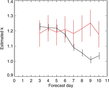
The automated technique was also used to explore the sensitivity of this k estimate to different choices of block size, hemisphere and forecast validity time. Block size mainly affects the size of the sampling errors, though at very small block sizes, e.g. 10 forecasts, the k estimates are significantly lower than those from the AR(2) estimate (e.g. 1.14±0.04). Appendix C speculates that very small blocks may naturally exhibit less autocorrelation due to the increasing dominance of the start and end samples. It is not possible to see any substantial difference between hemispheres, but for forecasts valid at day 8 and beyond, there may be a discrepancy between the autocorrelation approach and the non-parametric estimates, illustrated in Fig. 12. The autocorrelation estimates decline markedly at this forecast range (Fig. 4) leading to smaller estimated inflation factors, but the block method indicates a need to inflate the confidence range at all forecast validity times. At forecast days 3–7 we can be confident that temporal autocorrelation using an AR(2) model is sufficient to reproduce the inflation factors observed in the simulated null population. At days 8–10 there may yet be some unexplained property of the forecast scores, for example smaller but longer-range temporal correlations that are not modelled by AR(2) approach.

Fig. 12 Estimates of the inflation factor k for forecasts separated by 12 h made using the AR(2) technique with autocorrelations from Fig. 4 (black) or using the non-parametric technique applied to blocks of 30 paired differences from the explicit null population (red).

There remains the issue of how the inflation factor should be determined practically. Appendix C shows that estimates of the lag-1 and lag-2 autocorrelations from typical population sizes are affected by sampling error and that this propagates into quite large errors in the k estimate. For example, an estimate of k based on autocorrelation computed from 360 samples would have a 1-standard deviation range of ±0.09; for the 12 h data, that could mean that the inflation of the t-test confidence range could easily fluctuate between 12 and 31 % from one experiment to the next. Hence, unless the sample size is very big, as in this study, it is not reliable to generate autocorrelation estimates from the population under test. An alternative would be to use an explicitly generated null population, if available, to provide fixed estimates of k. These could be estimated either using the non-parametric CDF method of Fig. 4, or using the autoregressive method and a table of autocorrelation parameters estimated from the null population. However, the standard errors of the non-parametric approach are substantially larger than those from the autocorrelation approach, even after blocks from day 4 and day 10, SH and NH have been combined. Further, autocorrelation can be estimated for different hemispheres, different forecast times, and it can be extended to areas that this study has not examined, such as the stratosphere. The AR method makes it easier to tailor k to the situation and this approach is now being trialled in one of the ECMWF forecast verification packages, based on pre-tabulated autocorrelation estimates from the null population in this study. Any underestimate of the inflation factor at day-8 and beyond (e.g. Fig. 12) is of less practical consequence given how hard it is to show any statistical significance in changes in forecast quality at this range.

7. Correlations in forecast scores

So far the focus has been on RMS errors in 500-hPa geopotential height. It is also common to verify other dynamical fields (e.g. wind, temperature and relative humidity) and other vertical levels, from the surface to the stratosphere. Another popular measure of error is the anomaly correlation (AC or ACC, e.g. Jolliffe and Stephenson, 2012). 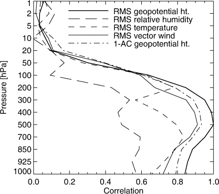Figure 13 shows linear correlations of the paired differences [d _i , eq. (33 )] from these scores against the day 5 RMS errors in 500-hPa geopotential height. These results are for the null distribution (perturbation minus control) but they would be the same for the AMSU-A denial (not shown). RMS geopotential scores are well-correlated across the troposphere though correlations decline towards the boundary layer and into the lower stratosphere. Anomaly correlation of geopotential height and RMS vector wind errors seem to bring little extra information — they are likely to be measuring rather similar kinds of errors in the large-scale synoptic patterns of the atmosphere (remember that the tropics are excluded from this study, where these scores might give more independent information). Only the RMS errors in relative humidity seem to be measuring something different, with around a 0.5 correlation to RMS errors in geopotential. A broad conclusion is that results based on geopotential height are likely to be replicated in any midlatitude medium-range score focused on tropospheric dynamics.

Fig. 13 Correlation of paired differences in NH day-5 RMS 500-hPa geopotential height error with paired differences in other measures of forecast error on the same forecast day for the same hemisphere. Anomaly correlation of geopotential height error (AC) has been transformed to (1-AC) to give positive rather than negative correlation.

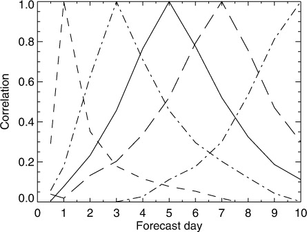
Forecast error differences are also correlated across forecast day. If one forecast is better than another at day 5, it is natural to expect the advantage to continue at day 6. That appears to be the case, but correlations across longer time ranges become quite weak. The correlations for RMS 500-hPa geopotential height error are shown in Fig. 14. The correlations of day-5 error differences (the solid line) drop to 0.1 or less at day 1 and day 10. Ignoring correlations less than 0.1, forecast error differences are correlated over about 2 days in the early forecast range and for 4–5 days in the medium range. Hence, even if one forecast is better than another at day 1, as measured by RMS error difference, this says nothing about the RMS differences in the medium range (at least as far as linear correlations are concerned). A hypothesis to explain this is that the large-scale synoptic errors that dominate the RMS errors in the medium or longer range have grown from much smaller, localised errors that are not an important contribution to the RMS errors at earlier ranges. Further, as has been shown, the daily variability of the paired RMS differences is dominated by chaotic variability.

Fig. 14 Correlation of paired differences in NH RMS 500-hPa geopotential height error across forecast day, for forecasts with the same base time. Examples shown for day 1, day 3, day 5, day 7 and day 10.

It is also interesting to look at the consistency of the averaged change in scores [, eq. (44 )] across forecast time. This analysis has to be performed on blocks of forecast scores like those in Fig. 10. Surprisingly, for blocks containing, for example, 60 or 230 samples, the correlations look a lot like Fig. 14 whether computed from the AMSU-A denial or the perturbation experiment (not shown). It should not be misunderstood from these results that initial condition error is not important in controlling the medium range error. Even small changes in the size of the initial condition error do affect the medium range, as can be shown when statistics are computed over long periods as exemplified by the AMSU-A denial in Fig. 5. However, the day-to-day variability in paired differences in forecast scores is dominated by chaotic variability in most typical experiments.

The effect of chaotic variability on forecast score correlations is best seen in Fig. 10. Panel a shows blocks from the AMSU-A denial experiment. Some blocks show an increase in RMS error across all forecast times, but with varying amplitude through the forecast range, likely due to sampling error. In panel b, the perturbation experiment does not show so much consistency across forecast time. However, results can still be consistent across 3–4 forecast days. It is tempting to think that if a few forecast days in a row show consistent changes in the scores, even if these changes are not statistically significant, that makes the results somehow more reliable. Such runs of consistent but not significant changes in scores can be generated by chaotic forecast variability.

Another aim of this correlation analysis has been to make an estimate of how many independent statistical tests are being made when we verify a full suite of scores across different hemispheres, different levels and different parameters. This will be particularly important later when trying to understand the impact of statistical multiplicity. Looking at the range over which linear correlations drop to 0.1, and excluding the tropics, stratosphere and early forecast range, there are only two uncorrelated tropospheric scores in one hemisphere: mid-range (day 3–6) and long-range (day 7–10). There is no correlation between paired differences in the SH and NH (not shown). We cannot necessarily assume that a lack of linear correlation indicates full statistical independence, but making that assumption would give a total of four independent scores.

8. Multiple comparisons

It has been shown that when the small temporal autocorrelation in paired differences is taken into account, an individual t-test is statistically robust. However, scientists often run multiple experiments and they usually look at more than one forecast score. So the issue of multiple comparison (multiplicity) can contribute to the excessive number of false positive results in forecast testing. The 95 % confidence range applies only to a single statistical test where it means there is only a 5 % chance of a type-I error (i.e. incorrectly rejecting the null hypothesis). However, once many tests have been made, the chance of a false positive becomes much greater. The issue of multiplicity is much better known in the medical sciences (e.g. Benjamini and Hochberg, 1995). In the atmospheric sciences, it has only received attention where it is most obvious, when trying to compute a significance test for each location in a latitude–longitude field (e.g. Livezey and Chen, 1983; Wilks, 2006). In forecast verification, the problem is most apparent when trying to compute changes in forecast scores as a function of latitude and pressure. Geer et al. (2010) found it was necessary to make a Bonferonni correction (e.g. Abdi, 2007) of the significance level from 95 to 99.8 % to counter the tendency to assign excessive statistical significance across one latitude–height diagram. There, an assumption was made that there were about 20 independent statistical tests being made across the diagram. It has to be recognised that the number of independent statistical tests is generally much less than the number of tests being made, as neighbouring points in a spatial field are usually correlated. Much of the difficulty of dealing with multiplicity is in trying to understand how independent the tests are and correcting appropriately.

The explicit null population can be used to demonstrate the effect of multiple comparisons on forecast testing, based on the 31 independent blocks of 60 forecasts. To gain extra samples, we combine what we assume are independent tests at day 4 and day 10, SH and NH, making 124 independent tests. Performing a t-test on each block using k=1.22 inflation, there are six rejections of the null hypothesis. We know the null hypothesis is true, so these rejections are incorrect, that is, type-I errors. The chance of type-I errors across multiple tests can be calculated using the binomial distribution as explained in Wilks (2006). Table 5 gives the probability of type-I errors for certain numbers of tests at 95 % confidence. For N=124 independent tests, we would have a 59 % probability of getting between four and seven type-I errors. Hence results computed from the explicit null population are consistent with statistical expectations. This also helps confirm the estimate from Section 7 that the NH and SH at day 4 and day 10 constitute four independent statistical tests. If they were all dependent, this would be an N=32 situation, but the presence of four or more type-I errors would be quite improbable in this case (see Table 5, only 0.07 probability). Further, had the same 132 tests been performed without inflation, that is, k=1, there would have been 14 type-I errors (not shown in the table, only 0.4 % probability). Hence, to control these false positives, it is necessary to inflate for autocorrelation and to understand the effect of multiple comparisons.

Table 5. The probability of a particular number of false results (type-I errors) being generated by N significance tests computed using a 95 % confidence range

	0	1	2	3	4	5	6	7
N=4	0.81	0.17	0.01	0.00	0.00	0.00	0.00	0.00
N=8	0.66	0.28	0.05	0.01	0.00	0.00	0.00	0.00
N=12	0.54	0.34	0.10	0.02	0.00	0.00	0.00	0.00
N=16	0.44	0.37	0.15	0.04	0.01	0.00	0.00	0.00
N=32	0.19	0.33	0.27	0.14	0.05	0.02	0.00	0.00
N=124	0.00	0.01	0.04	0.08	0.12	0.16	0.16	0.15

Generated from the binomial distribution following Wilks (2006). Bold type indicates the most probable number.

As far as hemispheric scores are concerned, it is unlikely to find so many independent tests being made in one scientific study (although there could be many times this number of tests being made across all the experiments being performed at one forecast centre.) However, even in a single study it is quite typical to examine the results from two or more experiments compared to a control. If there are about four different independent tests being made per experiment in the extratropical troposphere, across two experiments that would be N=8 independent tests. The table shows that at the 95 % confidence level there is a 34 % chance of one or more type-I errors across this testing, for example, roughly a 1 in 3 chance of a type-I error. If three experiments had been tested, that is, N=12, there would be a 1 in 2 chance of a type-I error. This clearly highlights the danger of ‘trawling’ — of experimenting with a variety of different strategies for improving an NWP system and picking the strategy that gives the apparently significant result.

The normal way to control multiplicity is the Šidák correction (e.g. Abdi, 2007) which seeks to control the type-I error rate across a whole ‘family’ of statistical tests. If a single test is at 95 % confidence and the null hypothesis is true, it has a c=0.95 chance of correctly confirming the null hypothesis. Given N independent tests, the chance of correctly confirming the null hypothesis in all of them is simply c ^N . If we want to set the ‘family-wise’ confidence interval to some value c _FAMILY , then the confidence range to be applied to each independent test, c _SIDAK , must be8 For example, if we want a 95 % family-wise confidence interval, that is, no more than a 5 % chance of a type-I error across two experiments compared to a control, with N=12, then c _FAMILY =0.95 and c _SIDAK =0.996. Each individual test must be made at a 99.6 % confidence level to give a 95 % confidence level across all testing. This affects the size of the confidence interval in eq. (66 ) through the t-distribution's z ₉₅ being replaced by the equivalent for a 99.6 % confidence level. In this example, the threshold z would increase from 1.96 to 2.87, giving a 46 % increase in the size of the confidence bars. Hence, in situations when several experiments are being compared together, the issue of multiple testing can become more important than that of temporal autocorrelation.

Applying the Šidák correction in this way, using an estimate of the number of independent tests in each experiment, appears a good strategy for controlling multiplicity in forecast testing. If rigorously applied in the forecast verification packages used for development testing at weather centres, this can help diminish the appeal of ‘trawling’ because the more hypotheses being tested at once, the lower will be the statistical power of any individual test. The more precisely formulated the hypothesis, the higher the statistical power available. For example, ‘better high orography screening for AMSU-A improves day-5 NH geopotential height errors’ is an N=1 hypothesis whereas ‘one of three possible new versions of the AMSU-A high orography screening will potentially improve forecast scores anywhere at any forecast range’ would be an N=12 hypothesis.

9. Minimum sample size needed for significance

It has been shown that paired differences in forecast quality between an experiment and control are dominated by chaotic variability in forecast error and that the real improvement from a typical scientific upgrade is a small signal on top of this. The inflated confidence limits (k=1.22, both with or without multiplicity correction) will be used to explore how this affects the size of sample required to verify a typical upgrade to an NWP system. As illustrated by the similarity of the distributions of paired differences from the perturbation and AMSU-A denial experiments (e.g. Fig. 6), the explicitly generated null population is valid for any experiment performed with the same forecasting system, so based on the standard deviations of the null population (Table 2) it is possible to predict the size of the 95 % confidence range for a typical experiment.

Figure 15 shows the results. It is hard to achieve statistical significance in short experiments unless a very large change is made to the quality of the forecasting system. Even without multiplicity correction, with 40 forecasts, the confidence range at day 5 would be ±2 %. It is rare to see genuine improvements of this size in medium-range forecast skill. One of the most significant developments in ECMWF history, the introduction of 3D-Var, generated improvements in day 5 errors of 5 % in the SH but just 1 % in the NH (Andersson et al., 1998). The example of removing (or adding) a single AMSU-A instrument is more typical, with its impact of around 0.5 %, and on average ECMWF scores are improving each year by about 2 %, based on dozens of different scientific contributions. As mentioned before, the problem is that we are typically making small developments in what is already a very good forecasting system. Though it can be illustrative to make experiments where, for example, the whole satellite observing system is discarded, such experiments do not precisely address the question of how to make progress.

Fig. 15 95 % confidence range for 500-hPa geopotential height in the NH, expressed as a percentage of the RMS error of the control, and as a function of the number of forecasts in the sample used to compute the scores: (a) without correction for multiplicity; (b) with an N=4 Šidák correction for multiplicity. If d ₉₅ is the range read from this figure, the full confidence range is ±d ₉₅.

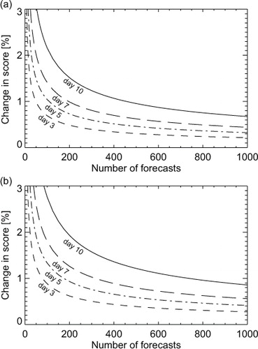
The ‘typical’ 0.5 % impact will begin to show statistical significance at day 5 with a sample of 424 forecasts, or 674 if N=4 multiplicity is taken into account. The extra cost of taking multiplicity into account should strongly motivate efforts to better design the experimentation and refine the hypotheses that are being tested, so as to reduce N. This result also suggests that even the recent ECMWF practice of demanding 6 months of testing for any proposed upgrade is likely to be insufficient (with two forecasts per day, this is about 360 forecasts in total). However, there is a greater problem of verifying scientific changes that have yet smaller impacts, particularly in preventing changes that make small degradations from entering the system. Even with 730 forecasts, a whole year of experimentation, at day 5 it would be impossible to distinguish a 0.2 % improvement from a 0.2 % degradation and in fact around 3000 forecasts would be required to give statistical significance. That is not a practical sample size: to create the 1880 forecasts used for the current work required a major effort that lasted nearly a year, that took advantage of the installation of a new supercomputer, and that was suspended during busy periods. For the longer-range scores, such as day 10, a real 0.5 % change in scores will not generate statistically significant results even with greater than 1000 forecasts, as illustrated in Fig. 5. There seems no justification for extending the forecast range used in the verification of typical experiments beyond 10 d, since very few results will be statistically meaningful.

Given that the temporal autocorrelation between paired differences requires us to inflate the confidence range, and this is worst when forecasts are made only 12 h apart, it might be thought better to verify forecasts spaced further apart, to minimise the autocorrelation and hence reduce the inflation required. However, this would be counterproductive, as shown in Table 6 (for simplicity concentrating on results without multiplicity correction.) Forecasts spaced 24 h apart still require a confidence range inflated using k=1.07. A 48 h spacing would probably remove all autocorrelation, which would allow the t-test to be used without inflation. The number of samples required to identify a 0.5 % change with statistical significance would reduce from 424 to 327 or 286 respectively. However, this can only be obtained with 327 or 572 d of data assimilation, as opposed to 212 if the forecasts are made every 12 h. The best choice depends on the relative computational cost of the forecast versus the data assimilation, but usually the cost of data assimilation is substantially greater. Hence it is most efficient to generate forecasts every 12 h but to inflate the confidence range accordingly.

Table 6. In order to give statistically significant results at 95% confidence range for a certain change in the NH 500-hPa geopotential height forecast sores at day 5, the top section shows the number of samples required, and the bottom section the number of days of experimentation required

Change in scores [%]	2	1	0.5	0.25
	Number of samples required
Forecasts every 12 h (k=1.22)	29	108	424	1690
Forecasts every 24 h (k=1.07)	23	84	327	1301
Forecasts every 48 h (k=1)	20	73	286	1136
	Days of experimentation
Forecasts every 12 h (k=1.22)	14	54	212	845
Forecasts every 24 h (k=1.07)	20	84	327	1301
Forecasts every 48 h (k=1)	40	146	572	2272

Results are shown using confidence limits inflated appropriately for forecast separations of 12, 24 and 48 h.

10. Conclusion

This study is a response to the difficulty of testing small improvements in forecast quality in the context of an already high-quality operational forecasting system. There is a natural desire among scientists to somehow ‘go beyond’ statistical significance and to draw inferences based on non-significant results. One aim of this study was simply to demonstrate how dangerous that is. The extent that chaotic variability affects forecast scores may not be fully appreciated. It has been shown how easy it is to generate apparently ‘statistically significant’ results by making a technical perturbation to a forecasting system, while keeping the science identical. However, even with statistical significance testing based on the Student's t-test, these happen more regularly than would be expected. In the differences between the technical perturbation experiment and the control, we would hope to generate very few statistically significant results, in line with the aim to have only 5 % chance of a false positive (type-I error); in fact using a simple t-test where no correction has been made for autocorrelation or multiplicity, we would generate false positives too frequently, confirming the anecdotal evidence that we are sometimes interpreting chaotic variability in NWP systems as a real scientific impact.

The need for a correction to the simple t-test has been demonstrated with an explicitly generated null population of thousands of paired forecast differences representing the true null population. Using a non-parametric technique in which the population is divided into contiguous, non-overlapping blocks and the t-test is applied to each block, it is demonstrated that an inflation factor of k=1.19±0.09 is required in the t-test for geopotential height scores at day 5, when forecasts are separated by 12 h. Non-Gaussianity has been ruled out as an explanation; the effect can be attributed to temporal autocorrelations in the paired differences as originally demonstrated by Fisher (1998). Using a good estimate of the null population's temporal autocorrelation, an autoregression model can be used to derive k without having to go to the trouble of applying the non-parametric approach on which this study is based. However, there are a number of important limitations to this approach:

• In the past, where autocorrelation corrections have been applied, they have been based on an AR(1) model. This is fine for forecast base times separated by 24 h but insufficient if the forecast base times are separated by 12 h, as has become increasingly popular. In that case, an AR(2) model is required.

• Estimates of the autocorrelation from the sample under test can be subject to substantial uncertainty. Using a Monte-Carlo approach, it has been shown that the k estimates based on AR(2) autocorrelation computed from 360 samples would have a standard error of ±0.09. Where possible, it is better to use fixed autocorrelation estimates derived from a much larger sample, such as the thousands of paired forecast differences used in this study, which brings the error down to ±0.02.

• At forecast days 8–10, the AR(2) model is not capable of reproducing the observed k inflation factors, which remain at around 1.2 while the autoregression model tends towards 1. A possible explanation is that small autocorrelations exist over much greater time ranges than are captured in the lag-1 and lag-2 autocorrelations treated by the AR(2) model. It may be difficult to make further progress understanding this issue, as any such correlations will be difficult to estimate accurately from the data.

• It is sometimes assumed that because forecast scores are correlated in time, it is safer to verify only forecasts that are well-separated, for example, to use only one forecast every 24 h, or indeed every 10 d. However, this is a poor strategy if testing involves running the data assimilation system, because it reduces the number of samples available without much reducing the cost of the testing, which is usually dominated by the assimilation component. With forecasts every 12 h, the confidence range needs to be inflated to take account of autocorrelation, but this is outweighed by the reduction in sampling uncertainty brought by the extra samples. It is always easier to detect changes in the quality of the forecasts using forecasts every 12 h than with a less frequent spacing.

The problem of multiplicity occurs when scientific studies examine the results from many different experiments and/or from many different scores. It is typical to generate an exhaustive set of forecast scores on many different levels and parameters, for different regions and views (e.g. zonal cross-sections and maps) and for different parameters, and this is vital for catching problems and for in-depth understanding of a forecast upgrade. Necessary as this is, it somewhat violates the scientific philosophy of making the hypothesis before performing the test, and it runs the risk of generating spurious results through multiplicity. However, for medium-range synoptic scores (ignoring the short-range, the tropics and the stratosphere) it has been estimated that there are only about four independent statistical tests being made in each experiment (in the mid-range, e.g. days 3–6, and the long-range, e.g. days 7–10, in the SH and NH). All dynamical scores are strongly correlated (whether computed as anomaly correlation or RMS, whether applied to geopotential, temperature or to the wind fields) and they are correlated across much of the troposphere. Changes in forecast scores are correlated from one forecast day to the next (even in the perturbation experiment) so even if a run of a few days appears statistically significant, this still counts as just a single result. Even before thinking about multiplicity, this suggests it is sufficient to pick, in advance, a set of scores that will represent these four independent tests, and on which the most rigorous statistical evaluation is to be based. However, there are still enough independent tests being made to cause problems of multiplicity. For example, when three experiments are being compared to a control, there are 12 independent tests of the medium-range synoptic scores being made. With a 95 % confidence range for the individual tests, that brings a 46 % chance of getting one or more false positives across all the synoptic testing. Hence, scientists should be sceptical of isolated results (e.g. without a correction for multiplicity, if forecast scores are improved only at day 4 in the SH in one of a set of three experiments, that should definitely be ignored). The recommended approach is to apply the Šidák correction based on an estimate of the number of independent tests being made.

Another aim of this study has been to give guidance on the sample sizes required to reliably test a small scientific change. Only the most significant developments demonstrate impacts on medium-range forecast scores of around 1–5 %, and something smaller is typical. The example here has been the 0.5 % change in scores resulting from the addition or removal of a single AMSU-A instrument (where six others are still assimilated). A steady flow of smaller changes like this has contributed significantly to the improvement of scores over the last few decades, and in any case, even the minor developments need scientific testing to prove they are not making scores worse. But to reliably test a 0.5 % change requires at least 400 forecasts, which would be computationally very expensive at any forecasting centre.

Are these results, based on perturbations to the ECMWF system, applicable to other forecasting centres? Apart from the sample size n, the size of the t-test confidence range is principally determined by the standard deviation of paired forecast differences s [refer to eq. (66 )] which can be seen as a measure of the chaotic divergence (the dynamical instability) of the forecast system under test. The corrections for autocorrelation and multiplicity make additional inflations on top of this basic confidence range. Recent results from continued testing with the ECMWF system also show that s may not be that constant, and that it may perhaps be affected by choices such as the resolution of the NWP system (recent testing done at the T639co resolution, equivalent to 15 km, gives s ≅3.16 m at day 5 compared to the s=1.62 m seen in the current experiments in Table 2). Further analysis of these new results will have to wait, but this suggests it would be necessary to check the s applicable to a particular forecasting system before determining the exact number of forecasts required to verify any particular level of impact. However, it is possible to estimate this reliably from a relatively small sample of paired forecast error differences. There may be some differences in magnitude when applied to other NWP systems, but the patterns shown in Fig. 15 are clear: it is very hard to distinguish small changes in forecast skill from the chaotic variability of a perturbed forecast system.

In the situation where traditional medium-range scores cannot always be used as a guide to the quality of scientific developments in forecasting, what do we do? We could just assume a priori that something that improves the science will improve the forecasts. However, bugs can creep into the system and science can be less well-understood than anticipated, so it is not realistic to abandon testing altogether. It is probably best to test fewer configurations but to do it more rigorously, generating many more samples and accepting the additional cost. A particularly wasteful strategy is that of making various minor changes to the system in various different experiments and then trying to decide between them using the forecast scores. This is basically ‘trawling’, and sets up a situation where the effect of multiplicity, unless corrected, will generate misleading results. One of the candidate developments may be chosen almost at random. Instead, it is better to carefully assess those minor changes before starting long forecast runs, and then to take just the best candidate forward into a full experiment. For example, when choosing among three different improved cloud screening schemes, it should be possible to find detailed evidence to distinguish the best among them (perhaps, in this case, by comparing to independent cloud retrievals.) Then the hypothesis that better cloud screening improves forecast scores can be taken forward in a single, long, high-quality forecast experiment.

There are a number of other strategies that may help. First, ensembles are one way to generate additional samples, though there are statistical challenges in interpreting the results and in generating confidence intervals. Second, in some cases, it might be appropriate to use substantially lower resolution for testing so as to generate more samples for less cost. However, the applicability of results from relatively low resolution compared to those from a full-resolution model requires confirmation. A third possibility is to concentrate on short-range forecast testing, where statistical significance is apparently easier to achieve. However, there are many pitfalls in short-range verification, particularly when using analyses as the reference, so often observation-based verification can be more reliable. Another issue with the short-range strategy (from the point of view of medium-range forecasting) is that it assumes that improvement in forecasts in the very short range will actually lead to improvement in the medium range. That is clearly true in general, averaged over many cases, but if it is only very small areas (whose locations change continuously) that control the growth of baroclinic errors, these areas are likely to get lost in hemispheric scores. Finally, innovative methods for diagnosing observation impact such as adjoint sensitivity (e.g. Baker and Daley, 2000) or ensemble spread (e.g. Harnisch et al., 2013) could be useful but because they are usually only applied to short-range verification, they face exactly the same issues. Short-range forecast verification has been excluded from the current study, but it is of great interest to understand it better. Overall, medium-range dynamical forecast scores remain the simplest, most direct and reliable tools for evaluating scientific improvements, but they do require sufficiently large samples along with rigorous statistical evaluation.

11. Acknowledgments

The following are thanked for assistance, discussions and reviews: Mike Fisher, Michael Rennie, Martin Janoušek, Elias Hólm, Roger Harbord, Stephen English and Erland Källén and an anonymous reviewer. Tomas Wilhelmsson and Deborah Salmond are acknowledged in their thankless task of controlling the numerical reproducibility of the forecasting system, which was essential in creating the perturbation experiment.

12. Appendix

A. Results using operational analysis as the reference

The results presented have been based on own-analysis verification. However, the entire study has been repeated using ECMWF operational analyses as the verification reference. The results are generally very similar and lead to very similar conclusions. Results and figures in Sections 3, 4 and 7 are nearly identical except for the changes in forecast scores in the early range (day 2 and earlier) of Fig. 5. Later sections rely on results that are themselves affected by sampling noise in their finer details. So where results are based on a limited number of blocks, details of the figures do differ with operational analysis as the reference, but all the conclusions are the same, including that the t-test is overly generous without an inflation of the confidence range of about k=1.22.

B. Creating the perturbation experiment

In the ECMWF assimilation system, two otherwise identical experiments will exhibit small numerical differences when the number of parallel processes is changed. In the variational data assimilation, observations and grid-points are distributed differently, and where floating-point summations are made across the results from different observations, they are made in a different order, resulting in very slight numerical differences at the level of precision of the 64-bit floating-point arithmetic. However, these small differences grow during the analysis process, resulting in visible differences between analyses, which also propagate through forecasts. There is a regularly maintained test procedure where the parallel distribution of observations is instead preserved and an option called LREPRO4DVAR is activated that recodes the key areas of code in ways that can preserve numerical reproducibility (such as doing sums using integer rather than floating-point arithmetic). This comes at additional computational expense, so it is only used for testing, and with these options set the ECMWF assimilation system is completely bit-reproducible when the number of parallel processes is changed. Because we can turn this numerical difference on and off, we can be confident that it is well understood and causes no knock-on bugs or other unknown scientific effects.

The areas that generate numerical differences in the analysis when different numbers of processors are used are the following:

• When computing the scalar product of the 4D-Var control variable.

• When computing the observational cost function.

• In the variational bias correction scheme, the accumulation of adjoint sums and the accumulation of bias predictor statistics.

• In the observation operator for all-sky microwave radiances, an optimisation that gives slightly different results depending on the exact order in which observations are processed.

• In the adjoint of the model-to-observation interpolation operator, which can sum adjoint contributions from many different observations onto the same model variables.

Experience shows that the source of the numerical perturbation is unimportant: any pair of experiments based on the same system and same resolution appear to exhibit a similar level of chaotic divergence, as demonstrated in this study by the very similar standard deviation of paired differences in the AMSU-A denial and the perturbation experiment.

C. Modelling variance inflation with autoregression models

Fisher (1998) and Wilks (2006) show how to specify an inflation factor k in eq. (66 ) to account for autocorrelation, under the condition that the autocorrelation can be modelled using an autoregression (AR) model. The day-5 NH 500-hPa geopotential height forecast score differences have a 12 h autocorrelation r ₁=0.15 and 24 h autocorrelation r ₂=0.07 (Fig. 4). Modelling this autocorrelation with an AR(2), k can be computed using:C1 C2 C3 C4 C5

The AR(1) solution can be obtained by setting r ₂=r ₁. A more general solution for any AR(N) can be found in Wilks (2006). For the NH example, k=1.22 which is quite similar to the implied inflation from the revised confidence limits suggested in Section 5. Rather than compute a null population explicitly, as is done in this work, it is possible to estimate the inflation factor directly from autocorrelation estimates of the population of paired forecast score differences, for example, Fig. 4. This enables the inflation factor to adapt flexibly to different forecast-spacings (e.g. every 12 h versus every 24 h) and to any variations there may be in different parameters and regions of the globe. The main problem is that estimates of autocorrelation are themselves subject to sampling uncertainty. Table 7 explores the effect of this on estimates of k using a similar Monte-Carlo method to that used to estimate the error bars for Fig. 4. For the typical sample sizes used in forecast verification, this will add considerable uncertainty to the estimates of the confidence ranges themselves. Only for very large samples, such as with the 1885 forecasts available in this study, does the estimate of k become reliable enough. Another interesting effect is that when small sample sizes are used, even beyond the large sampling error, the estimate of k has a clear low bias; this parallels the low bias in the non-parametric estimates of k in Section 6. A possible explanation is that the samples at the beginning and end of the block may contribute less to the autocorrelation and hence start to dominate the results.

Table 7. Sampling uncertainty of inflation factors k generated from autocorrelation parameters r ₁ and r ₂, which themselves have been estimated from a sample of finite size

Sample size	Mean	Std. dev.	Min	Max
Statistics of inflation factors generated from forecasts every 12 h (simulated by [0.025, 0.065, 0.82, 0.065, 0.025] convolution)
10	0.869	0.324	0.22	2.14
60	1.161	0.219	0.65	1.98
360	1.214	0.090	0.96	1.59
1885	1.223	0.038	1.11	1.35
Statistics of inflation factors generated from forecasts every 24 h (simulated by [0.035, 0.93, 0.035] convolution)
10	0.811	0.305	0.21	2.02
60	1.025	0.190	0.56	1.77
360	1.065	0.077	0.85	1.37
1885	1.071	0.033	0.98	1.17

A Monte-Carlo method is used: sequences of normally distributed random numbers are made autocorrelated by applying a convolution function; r ₁ and r ₂ are estimated and from these k is computed. 1000 randomly generated blocks of 10, 60, 360 or 1885 samples have been used.

D. Using bootstrapping to sample the null distribution

The results in the main study are limited by the number of samples that can be generated for comparison to the t-distribution whilst requiring contiguous and non-overlapping groups of forecasts. A larger set of samples could be computed using the moving block bootstrap resampling technique described by Wilks (2006). The basic unit is a small contiguous block of paired differences which is long enough to preserve most of the autocorrelation in the data but short enough to allow the population to be resampled in many different combinations. Here, a block length of four forecasts is used, which can be justified following Wilks (1997), based on the 0.15 autocorrelation between subsequent paired differences (from Section 3). These blocks are randomly drawn from the null population, with replacement, and assembled to create a sample of data from which a mean can be computed. Also, to gain the largest and cleanest sample, the four independent populations (NH and SH at day 4 and day 10, as used in Section 4) can be used. From each of the four null populations, 10 000 samples of size n are created by bootstrapping and their mean and standard deviation s are computed. These can be transformed into z-space via eq. (55 ). The results are shown in Fig. 16.

Fig. 16 (a) PDF of z-tests generated from bootstrapped samples of 720 forecasts (solid) and the Student's t-distribution (dashed). Based on a total 10 000 for each of the four independent populations.

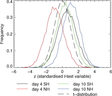
However, it looks like even bootstrapping cannot beat the limitations of a relatively small sample. For example, at day 10 in the NH, even over 1885 forecasts, the perturbation experiment has RMS errors that are on average 0.35 m larger than in the control (Table 2). This must be purely an effect of chaotic variability, as the experiments have no scientific differences. Bootstrapping creates a smoother histogram based on samples from these 1885 forecasts, but it can do nothing about these biases. Distributions like those in Fig. 9 can be generated but, although they are smoother, for the larger-size samples they are generally just as lopsided. Removing the bias would be incorrect, as that is part of the chaotic variability. There does not seem much to be gained from bootstrapping for the present work.

References

- Abdi H . Salkind N . The Bonferroni and Šidák corrections for multiple comparisons. Encylopedia of Measurement and Statistics. 2007; Sage, New York, USA. 103–107.
- Andersson E. , Haseler J. , Undén P. , Courtier P. , Kelly G. , co-authors . The ECMWF implementation of three-dimensional variational assimilation (3D-Var). III: Experimental results. Quart. J. Roy. Meteorol. Soc. 1998; 124: 1831–1860.
- Baker N. L. , Daley R . Observation and background adjoint sensitivity in the adaptive observation-targeting problem. Quart. J. Roy. Meteorol. Soc. 2000; 126(565): 1431–1454.
- Benjamini Y. , Hochberg Y . Controlling the false discovery rate: a practical and powerful approach to multiple testing. J. Roy. Stat. Soc. Series B. 1995; 57: 289–300.
- Bonavita M., Isaksen L., Hólm E., Fisher M. The evolution of the ECMWF hybrid data assimilation system. Quart. J. Roy. Meteorol. Soc. 2015; 142: 287–303. DOI: http://dx.doi.org/10.1002/qj.2652.
- Bowler N. , Cullen M. , Piccolo C . Verification against perturbed analyses and observations. Nonlinear Process. Geophys. 2015; 22(4): 403–411.
- Casati B. , Wilson L. , Stephenson D. , Nurmi P. , Ghelli A. , co-authors . Forecast verification: current status and future directions. Meteorol. Appl. 2008; 15(1): 3–18.
- Ebert E. , Wilson L. , Weigel A. , Mittermaier M. , Nurmi P. , co-authors . Progress and challenges in forecast verification. Meteorol. Appl. 2013; 20(2): 130–139.
- Fisher M . Statistical Significance Testing of Forecast Experiments. 1998. ECMWF Internal Memorandum R48.8/MF/30.
- Geer A. J., Baordo F., Bormann N., English S. All-Sky Assimilation of Microwave Humidity Sounders. 2014. ECMWF Tech. Memo. 741. Online at: http://www.ecmwf.int.
- Geer A. J. , Bauer P. , Lopez P . Direct 4D-Var assimilation of all-sky radiances: Part II. Assessment. Quart. J. Roy. Meteorol. Soc. 2010; 136: 1886–1905.
- Harnisch F. , Healy S. , Bauer P. , English S . Scaling of GNSS radio occultation impact with observation number using an ensemble of data assimilations. Mon. Wea. Rev. 2013; 141(12): 4395–4413.
- Hodyss D. , Majumdar S. J . The contamination of ‘data impact’ in global models by rapidly growing mesoscale instabilities. Quart. J. Roy. Meteorol. Soc. 2007; 133: 1865–1875.
- Isaksen L., Bonavita M., Buizza R., Fisher M., Haseler J., co-authors. Ensemble of Data Assimilations at ECMWF. 2010. ECMWF Tech. Memo. 636. Online at: www.ecmwf.int.
- Jolliffe I. T . Uncertainty and inference for verification measures. Wea. Forecasting. 2007; 22(3): 637–650.
- Jolliffe I. T. , Stephenson D. B . Forecast Verification: A Practitioner's Guide in Atmospheric Science. 2nd ed . 2012; Wiley, Chichester, UK.
- Livezey R. E. , Chen W. Y . Statistical field significance and its determination by Monte Carlo techniques. Mon. Wea. Rev. 1983; 111: 46–59.
- Lorenz E . Atmospheric predictability experiments with a large numerical model. Tellus. 1982; 34(6): 505–513.
- Lorenz E. N . Deterministic nonperiodic flow. J. Atmos. Sci. 1963; 20(2): 130–141.
- Magnusson L. , Källén E . Factors influencing skill improvements in the ECMWF forecasting system. Mon. Wea. Rev. 2013; 141(9): 3142–3153.
- Murphy A. H . Skill scores based on the mean square error and their relationships to the correlation coefficient. Mon. Wea. Rev. 1988; 116(12): 2417–2424.
- Radnoti G., Bauer P., McNally A., Cardinali C., Healy S., de Rosnay P. ECMWF Study on the Impact of Future Developments of the Space-Based Observing System on Numerical Weather Prediction. 2010. ECMWF Tech. Memo. 638. Online at: http://www.ecmwf.int.
- Robel J. NOAA KLM User's Guide (February 2009 revision). 2009. Online at: http://www.ncdc.noaa.gov/oa/pod-guide/ncdc/docs/intro.htm.
- Simmons A. , Hollingsworth A . Some aspects of the improvement in skill of numerical weather prediction. Quart. J. Roy. Meteorol. Soc. 2002; 128(580): 647–677.
- Student . The probable error of a mean. Biometrika. 1908; 6: 1–25.
- Thorpe A. , Bauer P. , Magnusson L. , Richardson D . An evaluation of recent performance of ECMWF's forecasts. ECMWF Newslett. 2013; 137: 15–18.
- von Storch H. , Zwiers F. W . Statistical Analysis in Climate Research. 1st ed . 1999; Cambridge University Press, Cambridge, UK.
- Wilks D . Resampling hypothesis tests for autocorrelated fields. J. Clim. 1997; 10(1): 65–82.
- Wilks D . Statistical Methods in the Atmospheric Sciences. 2nd ed . 2006; Academic Press, Burlington, MA, USA.