Internal variability of a 3-D ocean model

Abstract

The Defence Centre for Operational Oceanography runs operational forecasts for the Danish waters. The core setup is a 60-layer baroclinic circulation model based on the General Estuarine Transport Model code. At intervals, the model setup is tuned to improve ‘model skill’ and overall performance. It has been an area of concern that the uncertainty inherent to the stochastical/chaotic nature of the model is unknown. Thus, it is difficult to state with certainty that a particular setup is improved, even if the computed model skill increases. This issue also extends to the cases, where the model is tuned during an iterative process, where model results are fed back to improve model parameters, such as bathymetry.

An ensemble of identical model setups with slightly perturbed initial conditions is examined. It is found that the initial perturbation causes the models to deviate from each other exponentially fast, causing differences of several PSUs and several kelvin within a few days of simulation. The ensemble is run for a full year, and the long-term variability of salinity and temperature is found for different regions within the modelled area. Further, the developing time scale is estimated for each region, and great regional differences are found – in both variability and time scale. It is observed that periods with very high ensemble variability are typically short-term and spatially limited events.

A particular event is examined in detail to shed light on how the ensemble ‘behaves’ in periods with large internal model variability. It is found that the ensemble does not seem to follow any particular stochastic distribution: both the ensemble variability (standard deviation or range) as well as the ensemble distribution within that range seem to vary with time and place. Further, it is observed that a large spatial variability due to mesoscale features does not necessarily correlate to large ensemble variability. These findings bear impact on the way data assimilation should be addressed – especially in relation to operational forecasts.

• Baroclinic
• ensemble modelling
• salinity
• temperature
• elevation
• Skagerrak
• Baltic Sea

1. Introduction

For several decades, ensemble modelling has been an integral component of the meteorology forecasting process. During the data assimilation process, model ensembles may be constructed as perturbations on the initial conditions using schemes like ‘breeding of growing modes’ (see Toth and Kalnay, 1993), or singular modes (see for example, Molteni et al., 1996). The use of data assimilation is presently in wide use in ocean modelling, see for example, Shchepetkin and McWilliams (2005) and O'Dea et al. (2012). However, the use of ensemble models is less common. In some cases, the background error covariances are estimated using a ‘seasonal ensemble’ from a single multiannual model run, see for example, Oke et al. (2008). This, however, is not equivalent to running an ensemble of models.

As part of the MyOcean framework (EU research framework programme, FP7), Golbeck et al. (2015) presented several operational model setups for the North Sea–Baltic Sea region and join them in a cumulative ‘Multi Model Ensemble’ (MME). Although some of the individual setups employ data assimilation, none uses ensemble modelling. The common MME is available online in forecast mode and shows intramodel variability in time and space.

Some large-scale (basin to global) operational model systems do use ensemble members to produce ocean forecasts (Sakov et al., 2012; Brankart et al., 2015; Chu et al., 2015). There, ensemble members are generated by perturbing the physical state in the ocean or by using ensemble atmospheric forcing. For hindcast studies, a number of ensemble model studies have been made. For instance, Melsom (2005) studied the mesoscale variability along the Norwegian coast, using eight ensemble members that were generated by perturbing the initial field in a HYCOM model setup. Furthermore, Holt et al. (2011) used a coupled ocean–atmosphere mesoscale ensemble (33 members) system to provide uncertainty information for tropical cyclones.

The most common variable to assimilate seems to be sea surface temperature (SST) from satellites. However, assimilation of SST may have only a minor effect on the model result for Skagerrak and Kattegat, our area of interest, since the baroclinic features in these regions are mainly governed by salinity differences, see for example, Gustafsson (1999) and Nielsen (2005). For the North Sea–Baltic Sea regional domain, Fu et al. (2011) showed in a model study that there is a positive effect when including assimilated T/S profiles. They found the effect to be ‘persistent for nearly 3 weeks’ for their setup running in hindcast mode. A much shorter time scale is reported by Losa et al. (2012), where assimilation of SST in the North Sea leads to improvements for ‘up to 5 days’ in a pre-operational model.

The actual location of the mesoscale features may be important to the users of operational forecasts, as the positions of eddies and fronts in some areas have significant impact on, say, surface velocities. This has a direct influence on, for example, search-and-rescue operations (e.g. Melsom et al., 2012), oil drift forecasting used for environmental protection (e.g. Broström et al., 2011) and ship routing (e.g. Chu et al., 2015).

This article will examine in detail some of the uncertainties related to pure stochastical/random phenomena within a single numerical experiment. The purpose is to shed light on some of the inner workings of the model, prior to a decision on how to refine the model setup using data assimilation and ensemble modelling. In the present work, the term ‘Internal Model Variability’ denotes the variation within a numerical (hydrodynamic) model due to effects such as numerical round-off, that is, effects which are unrelated to the model parameter settings, physical forcing and boundary conditions. Golbeck et al. (2015) compared results from different models originating from various operational centres in northern Europe. The study examined the results for the North Sea and Skagerrak for a 1-yr period, and a significant spread in the model results was observed. In Skagerrak, the yearly average of the ensemble standard deviation of the sea surface salinity was found to be about 3–4 PSU. However, it was not examined how much of the variability that is due only to the stochastic nature of the individual models (ensemble members). We conjecture that the internal model variability is a key element in understanding how the model works, and, for example, to determine if a model change gives a significantly improved result. Also, the internal variability is important in the setup of ensemble models and in the interpretation of the results from ensemble systems.

2. On numerical models and stochastic (random) processes

The physical processes of hydrodynamics inherently contain a stochastic component caused by the turbulent nature of the flow processes. The end result is that for any given initial state and forcing, there is not a single determinable path of the system – it is chaotic in nature, see for example, Lamb (1932). This does not mean that the processes are entirely unpredictable, but rather that the exact physical state cannot be predicted in advance, see for example, Lorenz (1963). It may be predicted that there will be a number of eddies, swirls or gyres, but the exact path of each eddy is not possible to determine in advance. In some sense, the physical system may be seen as a stochastic process, which is executed only once.

A numerical model, which accurately describes the physical processes, will – at least to some degree – share the stochastic nature of the flow. If the transient nature of the flow is to be predicted, then the experiment must simulate each eddy (on the chosen scale). Although a particular numerical result may be reproduced exactly by re-running the experiment, it is still so that the result should be seen as a single outcome of a stochastic process. If the simulation is perturbed just slightly, then it may result in a rather different end result. If the perturbation is small enough, then the overall model stochastic process is not changed, and the second simulation may be viewed as a second outcome of the same stochastic process.

At FCOO (Defence Centre for Operational Oceanography), it is often necessary to go over each model setup to see if it can be improved. Normally, each candidate setup is then simulated for several years of hindcast, and a statistical analysis comparing model data with observations is performed to evaluate the model skills. The model skills, such as explained variance, of the various model setups are then compared to determine which model setup is ‘the best’. However, as each numerical experiment should be seen as a stochastic process, it may not be possible to determine which of the model setups on average give the best result. In principle, each experiment ought to be run several – or tens of – times to get an estimate for the statistical properties. Then, those properties could be compared between the various setups and the ‘best’ setup could be chosen. In practice, however, this method would be very cumbersome with respect to compute resources, as several years of hindcast should be computed for several setups and the whole thing repeated many times.

2.1. Simulation perturbation: branching

The ocean circulation forecasts made at FCOO are based on the GETM (General Estuarine Transport Model; Burchard and Bolding, 2002) code. The model has a very good track record for the North Sea–Baltic Sea transition zone, see for example, Holtermann et al. (2014), which is a key area for FCOO. As the numerical experiments themselves are repeatable, it is necessary to, in some sense, perturb (‘push’ or ‘nudge’) in order to trigger a branching or bifurcation into different stochastic outcomes. There are surely many different ways to trigger a branching. However, it seems imperative that the perturbation is so small that it does not represent a significant physical change. In some sense, the perturbation must be (much) smaller than the accuracy with which the perturbed quantity is known, such that the perturbed quantity is not less accurate than the unperturbed quantity.

After a quantity is perturbed, simple numerical arithmetic, such as round-off or truncation errors, may increase the differences over time. This effect may depend on how diffusive the processes are – some numerical processes may actually converge back to a stable equilibrium if the perturbation is small enough. The present study will try to shed light on the following topics:

• How large an initial change (perturbation) is needed to trigger a branching?

• How fast do the changes grow after a branching?

• How long does it take branched simulations to ‘grow apart’, that is, so the physical states vary?

• How large is the maximum/long-term variation between branched simulations?

It may a priori be expected that the initial growth of differences could be roughly exponential. This behaviour is in accordance with the theory for dynamic systems, where close trajectories diverge exponentially fast if the so-called Lyapunov coefficient is positive, that is, if the system is chaotic. There must be a limit for how large the differences (variability) can be, as the local (in time and space) salinity variations indicate some limit for the maximum possible variability between ensemble members.

In the present study, we perturb the 3-D GETM hotstart files, that is, the initial conditions. The salinity of each vertical column is updated by adding a small value, , to each cell of the column. As the salinity of each water column is perturbed, the vertical stability of the column should not be affected except in very special cases. It must be ensured that the update does not result in negative salinities. However, as the examined model setup uses a minimum salinity of 0.01 PSU (corresponding to freshwater runoff), this requirement should be met, as long as the random constant is numerically much smaller than 0.01 PSU.

In the present study, the perturbation is implemented as a scale multiplied by a random component, that is, , where is a scale of unit PSU, and each p(x,y) is randomly chosen from a uniform distribution over the interval [−0.5: 0.5[. Here, and in the following, (x,y) denotes the horizontal spatial coordinates, typically longitude and latitude. It may be noted that the perturbations in the present study are not chosen to maximize the initial growth of ensemble modes, see for example, Toth and Kalnay (1993), as might often be of practical usage in ensemble modelling.

As p is symmetric about zero, the average salinity change should be close to zero. The seed, p(x,y), and range, , can be chosen uniquely and independently. Therefore, it is possible to create perturbations, which are ‘in the same direction’ (identical seed), but with different magnitudes (scale). In addition, the scale can be chosen to be absolute (a specified range in PSU), or be relative to the local (maximum of) salinity in each water column.

2.2. Statistical ensemble variability measures

To assess the model variability, a number of independent simulations are made. In the following, z and t denote, respectively, the vertical coordinate and time. Each simulation in an N-member ensemble is denoted by an integer, n, where 1⩽n⩽N. If the nth ensemble value of a quantity f is denoted by f _n , then the average of f is defined as the simple mean over ensemble members:1 Similarly, the standard deviation, denoted as STDDEV, is computed straightforward as2 The surface salinity standard deviation is denoted as σ _SS. In some cases, the range of the ensemble is examined, where range is computed as3

In some sense, RANGE may be considered the ‘maximum variability’ within the chosen ensemble. However, as RANGE is computed based on (max – min), it really takes into account only the two most extreme ensemble members at each time step. The present study will use N=20, and it may easily be shown that for a 20-member ensemble, RANGE must be within two to roughly six times STDDEV, depending on the distribution of the ensemble. Thus, RANGE may also be used as a measure of the variability.

The simulations are perturbed at a particular point in time (t=0). Thus, at t=0, the variability is limited to the perturbation applied. For large values of t, the standard deviation may fluctuate but is not expected to increase in general. The actual values of the ‘limit’ are expected to depend strongly on the location, and on how much the natural variability of the variable is at that location. This includes phenomena like gradients across fronts and strength and size of local eddies.

3. The FCOO model setup

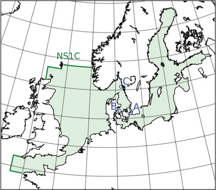
In this study, the FCOO operational GETM setup ‘NS1C’ (Büchmann et al., 2011) is examined. It is a 60-layer, 1 nautical mile resolution setup covering the North Sea–Baltic Sea area, see Fig. 1. Prior to the present experiments, which start on 2013-01-01, the operational setup has been run in a hindcast mode for the 3 yrs (2010–2012).

Fig. 1 FCOO NS1C model setup. Data comparison positions are marked for clarity: Drogden (A) at (longitude; latitude)=(12.7117; 55.5358), Ballen (B) at (10.6444; 55.8167) and Å13 (C) at (11.0333, 58.3367).

The present version of the NS1C setup uses MPI parallelization with 261 subdomains, each of size 66 × 30 in the horizontal. The advection schemes are first-order monotone for velocities, and TVD (third-order monotone) for salinity and temperature. The turbulence is parameterised using a second-order κ–ɛ model implemented under the GOTM (General Ocean Turbulence Model) framework, see Umlauf and Burchard (2005). The lateral boundary conditions of the NS1C setup are obtained from a coarser 2-D/barotropic model of the North Atlantic (NA3) and a tidal signal using the OSU tidal inversion (Egbert and Erofeeva, 2002) with a newer high-resolution data set (COAS, 2015). Boundary conditions for salinity and temperature are computed by interpolation of a monthly climatology. Meteorological forcing is from HIRLAM (Undén et al., 2002) S03, 3 km resolution, hourly fields, provided by the Danish Meteorological Institute (DMI). Freshwater fluxes are computed from daily forecasts from the HBV model (Lindström et al., 1997), provided by the Swedish Meteorological and Hydrological Institute (SMHI) and from observational data provided by the German Federal Maritime and Hydrographic Agency (BSH).

In Fig. 1, the positions ‘Drogden’, ‘Ballen’ and ‘Å13’, which are used for data comparison in the present study, are shown. The positions all lie in the difficult transition area between the North Sea and the Baltic Sea.

In the FCOO operational setup, a higher resolution 600 m model (DK600) covers the inner Danish waters, that is, the transitional zone between the North Sea and the Baltic Sea. At FCOO, the operational setups (NA3, NS1C and DK600) are executed operationally four times per day, providing 54-h forecast data used for, for example, search-and-rescue operations, low sea-level warnings, and oil-drift analyses. In addition, the forecasts are provided as a service to the general public.

4. Experiment A: branching and repeatability

For the initial test (experiment A), a short 5-d simulation experiment is undertaken starting at the perturbation date 2013-01-01.

For standard double precision arithmetic (64-bit, 53-bit mantissa), the relative accuracy (machine epsilon) is around 1.1 × 10⁻¹⁶. Thus, to actually perturb a salinity value of around 35 PSU, an update of at least 4 × 10⁻¹⁵ PSU must be made. For the case where , the typical update is of magnitude 2.5 × 10⁻¹⁵ PSU, so for many water columns in the North Sea, there will be zero perturbation in this case. As the perturbation scale is decreased to 10⁻¹⁴ PSU and below, the largest salinity values are no longer modified, and a subset of subdomains have unmodified hotstart files. At a scale of 10⁻¹⁸ PSU, even the smallest salinity values are no longer changed. In such cases, the hotstart files are identical to the baseline experiment, and the ‘perturbation’ ends up being just a repetition of the unperturbed baseline experiment.

In addition to the zero-perturbation ‘baseline’ experiment, perturbations have been made with changing by a factors of 10 from 10⁻⁴ PSU down to 10⁻¹⁸ PSU.

The actual amount of salt redistributed in each perturbation, that is, the volume of positive salt added to approximately half the cells, can be estimated as4 where p _max=0.5 is the maximum value of the positive half of uniform distribution [0:0.5[, N _cells is the number of water columns in the model, A _cell and D _avg are, respectively, the average surface area and depth of the columns. An equivalent amount of salt is removed from other columns, thus the word ‘re-distribution’. As an example, the salt redistribution for may be estimated asThe computations for from 10⁻⁴ PSU down to 10⁻¹⁴ PSU are completely equivalent and can be scaled by their exponent, that is, roughly 100 g of salt is redistributed with 10⁻¹⁴ PSU.

Perturbations have also been made, where the perturbation scale is a set fraction of the maximum salinity in the water column to be updated. Here, relative values ranging from 10⁻¹⁵ and down to 10⁻¹⁹ have been examined. The smallest value again corresponds to a pathological zero update of the initial conditions, resulting in a repetition of the baseline experiment. For a relative scale of 10⁻¹⁸, only the upper part of a single water column is actually updated, and the total amount of salt change is <1 µg in this case. Even so, simulation branching is observed both for this and all other cases where a non-pathological change of the hotstart files have been made. Thus, for the present case, any actual modification of the initial salinity – no matter how small – has resulted in a simulation branching.

5. Experiment B: realistic independent ensemble

As even the smallest change to the hotstart files (initial conditions) leads to a simulation branching, a very small perturbation scale is chosen for the following experiment. It is, however, prudent to have a very large number of possible perturbations. Therefore, the perturbation scale is chosen large enough, so that the salinity may be changed in all vertical columns. Further, the change to a single column should not just have one or two discrete possible perturbations, but many (preferably at least a few hundreds). A perturbation scale of 10⁻¹² PSU ensures that there will be hundreds of possible permutations for each water column – even in high-salinity waters. As a consequence, the perturbation of Experiment B is chosen with scale (absolute value). On a side note, this means that approximate 10 kg of salt is redistributed over the entire volume of the North Sea and Baltic Sea, compared to teratons of total salt in the area. The seed for each ensemble member is saved to file for possible later rerun of the experiment.

For Experiment B, 20 independent perturbations are made from the baseline experiment to give a reasonable ensemble size. Each ensemble member is started at the perturbation date (2013-01-01) and is run for 1 yr. The first 2 d have been simulated with output in double-precision NetCDF and with a higher output frequency (every 15th minute) for 3-D data. The added precision is necessary in order to compute statistics of the very small variations of the initial ensemble.

5.1. Results after first week of simulation

In Fig. 2, the RANGE of the elevation at a particular position is depicted. It should be noticed that the RANGE starts at O(10⁻¹⁴) m and increases rapidly up to a few tenths of a millimetre over the first few days simulated. It is noted from Fig. 2 that the computed ratio between RANGE and STDDEV falls within the limits of approximately 2–6 expected for a 20-member ensemble.

Fig. 2 Elevation RANGE (max − min results) at position ‘Ballen’, see Fig. 1 for position. Also shown is the ratio RANGE/STDDEV, where RANGE and STDDEV are computed over the 20 ensemble members.

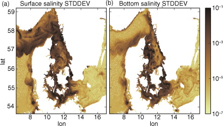
In Fig. 3, the ensemble salinity standard deviation is depicted after 5 d of simulation. At this point, the model output is in single precision, so the minimum differences of O(10⁻⁷) m or lower corresponds to machine accuracy on the output. In a few days, STDDEV grows by 10–11 orders of magnitude in many areas.

Fig. 3 Salinity variation (PSU) (STDDEV over 20 ensemble members) at surface (a) and bottom (b) after 5 d of simulation.

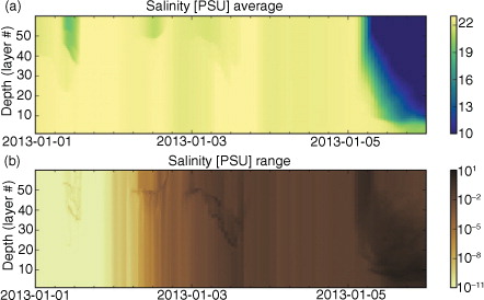
The salinity variation at Drogden Sill is shown in Figs. 4 and 5. As expected, the initial RANGE corresponds to the applied level of perturbation. However, after a few hours, the variation grows very fast. An exponential increase of 10 orders of magnitude in 34 h (about 7 orders of magnitude per day) is shown for reference in Fig. 4. On 2013-01-05, after the initial exponential growth, an outflow of brackish Baltic Sea water is visible in the data, see Fig. 5a. It is interesting that the maximum ensemble variability for salinity for this episodic event does not occur at the surface nor at the bottom, but rather in the halocline, see Fig. 5b, where for a brief period RANGE reaches a maximum of 5.8 PSU (maximum standard deviation 1.5 PSU). The fast development of the ensemble variability is not unique to the Drogden Sill, a similar development can be observed at other positions. Not surprisingly, the initial variability is consistently around 10⁻¹² PSU for all examined positions, corresponding to the initial perturbation level. At position ‘Å13’ in the eastern Skagerrak, see Fig. 1, sea surface salinity RANGE grows from roughly 10⁻¹² to 10⁻⁵ in about 13 h, corresponding to a growth rate of about 13 orders of magnitude per day (results not shown). Thus, although the exponential growth rate varies in the model area, similar behaviours are observed throughout the system: a few hours with very little variability variation – probably just a re-balancing of the system after the perturbation, followed by a rapid exponential growth for about 1–2 d. Finally, a slower increase in the variability can be observed, as the ensemble develops towards a saturated state.

Fig. 4 Surface salinity RANGE (max − min over 20 ensemble members) time series at the Drogden Sill (the Sound).

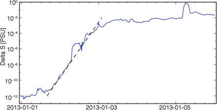
Fig. 5 Time-depth diagram of ensemble salinity AVG (a) and RANGE (b) at the Drogden Sill (the Sound). Water depth at the sill is approximately 8 m.

5.2. Variation growth anomalies

The time series of standard deviation within the ensemble members have been studied carefully, and it has been noted that there are sporadic ‘jumps’ in the data, that is, times where the difference between the simulations increases very rapidly in a single point. This effect is particularly noticeable in log-scale animations of the development of the standard deviation over the first days.

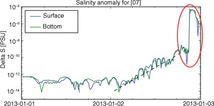
Figures 6 and 7 highlight one particular jump occurring in the German Bight after nearly 2 d of simulation. In Fig. 6b, the location of the jump stands out clearly on the ‘background’ standard deviation. There are no signs of this feature just 15 min earlier in the simulation, see Fig. 6a. The bottom salinity variation is very similar to the depicted surface variation (results not shown). A closer inspection of the data has revealed that just a single ensemble member (#07) of the 20 stands out from the rest. In Fig. 7, the absolute value of the salinity anomaly of this single simulation is shown. The anomaly is computed as the difference between the salinity of the chosen simulation and the average of the other 19 ensemble members. To gauge the initial growth rate, a dashed line with a constant growth of six orders of magnitude per day is shown for comparison. From Fig. 7, it is noted that there is an apparent instantaneous increase in the anomaly by about five orders of magnitude from 4.1×10⁻¹⁰ to 5.6×10⁻⁵ PSU. Just after the jump, the sign of the anomaly (not shown) is positive at the surface and negative at the bottom. In other words, after the jump the salinity gradient from surface to bottom is slightly larger for simulation #07 than for the other 19 ensemble members. These jumps seem to occur only relatively rarely in time and space, and only for the first days of the simulation, after which the general variability is so large as to hide the difference occurring from a single jump.

Fig. 6 Surface salinity variability (PSU) before (a) and after (b) a discrete ‘jump’ in a single ensemble member.

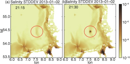
Fig. 7 Absolute value of the salinity anomaly of simulation #07 at (longitude, latitude)=(7.569, 54.441).

The mechanics of the jump can be explained by the vertical advection scheme in GETM, which has an (optional) iterative process to ensure the stability of the scheme. The number of iterations involves the computation of a round-up (ceil-function) on a floating point variable. This means that even a small variation in the floating point value may change the number of iterations, which again may trigger a relatively large difference in the result. As a consequence, initial almost identical simulations may drift apart ‘slowly everywhere’ due to the numerical differences of the slightly perturbed data undergoing identical instructions, and ‘sudden sporadically’ due to the occasional differences in the number of iterations in some of the computations, that is, differing instructions. It should be noted that the observed discrepancies in, for example, salinity from a change of the iteration count have been small – less than 10⁻⁴ PSU – much smaller than the typical error of the model. Further, one extra iteration step in the vertical iteration does not necessarily yield a higher accuracy of the end result. Hence, in the case mentioned above, simulation #07 is not better or worse than the rest. It is just different.

5.3. Spatial distribution of ensemble variability

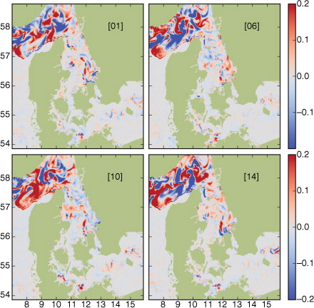
Previously, see Figs. 4 and 5, it was shown that the salinity variability at the Drogden Sill increases to O (1) PSU within a few days of simulation. A similar increase takes place in many other parts of the domain, but both the rate of increase and the final size may vary with space. If the surface salinity of the individual ensemble members is examined after a few months of simulation, see Fig. 8, then it may be noted that they have a lot of overall features in common. For instance, the members all show mesoscale eddies in Skagerrak and a north–south oriented front in the central Kattegat. Also, salinity gradients of several PSU across fronts seem consistent features. Common frontal features can be observed also north of the Sound and along the German coast in the western Baltic Sea. However, a more detailed inspection of the images in Fig. 8 reveals that the exact locations and shapes of eddies and fronts differ among the simulations. Noticeably, the shapes of the eddies in central Skagerrak (latitude=58° N, longitude=9.5°E) differ between members #6, #10 and #14. The ensemble-averaged surface salinity exhibits the same large-scale spatial variability as the individual ensemble members (results not shown), that is, with the high values of about 35 PSU in western Skagerrak and down to about 8 PSU in the western Baltic Sea. A priori, the largest ensemble variability may be expected to occur in regions with strong salinity gradients, which for date 2013-03-01 is in the German Bight, in Skagerrak, and in the northwestern and central Kattegat regions (Fig. 8). In practice, however, large anomalies from ensemble average are found in Skagerrak and near the front in central and north western Kattegat, but not in German Bight, see Fig. 9.

Fig. 8 Surface salinity (PSU) for 4 of 20 ensemble members after 2 months of simulation (2013-03-01).

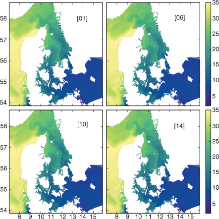
Fig. 9 Salinity anomaly (PSU) for 4 of the 20 members after 2 months of simulation (2013-03-01).

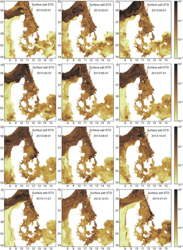
In Fig. 10, snapshots of σ _SS are shown for the first day of each month throughout the simulated period. There are many regions where the variation covers several orders of magnitude, either temporally from one time frame (month) to the next or spatially within a time frame. During the first month of simulation, σ _SS increases from O(10⁻¹²) PSU to above O(10⁻³) PSU on most locations, see Fig. 10a. It is worth to notice that the variability in the surface salinity does not continue to increase beyond the first few months. This suggests that 1 yr simulation period should be sufficiently long to reach a saturated state for the internal variability of the surface salinity. From Fig. 10, it is noted that the highest ensemble standard deviations are found in frontal zones and eddies in Skagerrak and Kattegat. Also, there seems to be some hotspots for variability in the Danish Straits and western Baltic Sea. It must be noticed that for a few locations, there is relatively high variability at the end of simulation. For instance, east of Bornholm (Fig. 10l), σ _SS is above 0.1 PSU on 2014-01-01. For that region, that is a rather high ensemble variability, the spatial variability of the salinity within each member is less than about 1 PSU in that particular region. However, from the present data set, it is not readily possible to determine if the high variability is due to initial effects, seasonal effects or just plain random stochastics.

Fig. 10 Surface salinity STDDEV (PSU), σ _SS, over 20 ensemble members at 1-month time interval.

There are even higher σ _SS values between these 12 dates. The temporal maximum of σ _SS, see Fig. 11a, shows irregular features with strong gradients. This suggests that the events responsible for the maxima are local phenomena such as strong fronts. If the position of a front differs between the ensemble members, then it is only during a short period and in this local area that there will be high values of σ _SS. Before and after the frontal passage, the values will be much lower. The maximum values in σ _SS in Skagerrak, eastern Kattegat and the southern part of the Sound are several PSUs, and about one PSU on some locations in western Kattegat, western Baltic Sea and German Bight. Even though fronts frequently occur in the southwestern Kattegat and the Great Belt, the maximum σ _SS is about one order of magnitude lower in these areas. This might seem surprising or even counterintuitive, but it might simply indicates that fronts in the Great Belt are more deterministic in nature than, for example, eddies in Skagerrak.

Fig. 11 Maximum surface salinity STDDEV (PSU) over time (a) and time-average (b) as well as time-maximum (c) and time-average (d) bottom salinity standard deviation over time for the 12-month simulation. Computations based on hourly values of salinity.

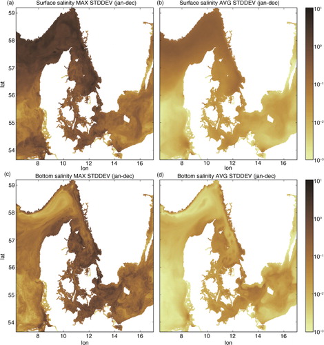
In general, the temporally averaged σ _SS, see Fig. 11b, is about one order of magnitude smaller than the maximum values. Further, the temporally averaged field is much smoother than the field of annual maximum values. The large difference in magnitude between these two fields indicates that the large values are reasonably rare events, with longer periods of modest variability in between. It is worth to notice that certain areas, such as the German Bight and the western Baltic Sea, stand out with especially high ratio between maximum σ _SS and time-averaged σ _SS values. It is concluded that high-variability events are rarer in these particular areas than in, say, Skagerrak.

The distribution of bottom salinity ensemble standard deviation (σ _SB) differs significantly from σ _SS. The temporal maximum and time averaged values of σ _SB over the simulated year are shown in Fig. 11c and d. It is immediately noted that there are very low values of σ _SB in the deeper areas of Skagerrak and Kattegat. In these areas, the bottom is dominated by high-saline oceanic water with little salinity variation in time and space, which could explain the limited ensemble variability. In other areas, such as the eastern Kattegat near the Swedish coast, the western Baltic and the Arkona Basin, there are relatively deep areas (depth>20 m) that have significantly higher values of σ _SB. In these areas, it is expected that there are significantly more activities, saline inflows, etc., which lead to higher variations in the ensemble. Finally, it should be mentioned that the values of σ _SB above 1 PSU are observed in areas where upwelling frequently occurs, such as southern and western Kattegat. As observed for the surface layer, high maximum values and relatively low averaged value are present in the German Bight and parts of western Baltic Sea. It should in this context be noted that only the surface and bottom field are analysed here. There may be even higher maximum and average ensemble standard deviations within the water column.

5.4. Ensemble variability in different areas

The ensemble variability of salt and temperature varies significantly between the various areas shown in Fig. 12. Further, there is a large difference between the maximum variability in an area and the average variability over the area. Also, for several areas, there is a large difference between variability at the surface and at the bottom. To quantify the long-term variability, the time average over the final 4 months of simulation, that is, September–December, is computed for each region. It is thus assumed that the ensemble have reached some steady state for variability within the first 8 months of simulation. As we shall see, this may not be the case for all areas, but that will be dealt with later.

Fig. 12 Regions to compute time evolution of averaged and maximum standard deviation of salinity and temperature.

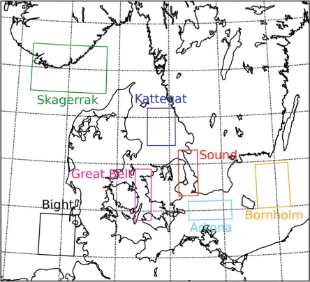
From Table 1, it is noted that the long-term regional maximum variability (STDDEV) is typically significantly larger than the regionally averaged values, by roughly one order of magnitude. Together the two numbers may provide a good indication of the typical variability for the variables in a particular area. It should be noted, though, that the values in Table 1 may be sensitive to the actual period chosen for the temporal averaging, both to the start and the length of the period. In particular, the start of the period should be late enough to be after any initial effects due to the model branching, and the length should be sufficiently large to yield an accurate average value. As both start and length of the period could be chosen differently, the values in Table 1, should be taken as orders of magnitude only.

Table 1. Computed long-term ensemble variability for salinity and temperature for different areas

		STDDEV salt (PSU)				STDDEV temperature (°C)
	Depth (m)	Surface		Bottom		Surface		Bottom
	Avg (area)	Avg (area)	Max (area)	Avg (area)	Max (area)	Avg (area)	Max (area)	Avg (area)	Max (area)
Skagerrak	290	1.4E-01	7.4E-01	7.2E-03	1.6E-01	7.9E-02	4.5E-01	3.1E-02	3.1E-01
Kattegat	28	5.7E-02	5.3E-01	3.8E-02	6.9E-01	2.2E-02	1.8E-01	4.9E-02	3.4E-01
The Sound	12	4.2E-02	4.4E-01	5.8E-02	8.9E-01	1.7E-02	2.4E-01	2.1E-02	1.8E-01
Arkona	39	1.9E-02	1.5E-01	4.7E-02	5.0E-01	2.1E-02	1.3E-01	3.6E-02	3.5E-01
Great Belt	17	2.2E-02	2.3E-01	2.2E-02	3.3E-01	6.8E-03	1.3E-01	7.6E-03	8.9E-02
Bornholm	72	1.8E-02	8.1E-02	2.3E-02	1.9E-01	3.7E-02	2.3E-01	4.9E-02	3.8E-01
German Bight	22	6.7E-03	8.5E-02	4.6E-03	7.0E-02	3.2E-03	3.8E-02	2.7E-03	2.3E-02

Regional average and maximum values of STDDEV have been temporally averaged over the final 4 months of simulations. Average depth of each region is given for reference.

The data in Table 1 may be used to identify some rather different stochastic regimes. In particular, Skagerrak and the German Bight are areas where the surface salinity within each ensemble member varies significantly in both time and space. In Skagerrak, the variation is typically 28–34 PSU, while the chosen area of the German Bight experiences values around 24–34 PSU, see for example, Fig. 8. However, the ensemble variation is more than an order of magnitude larger for Skagerrak than for the German Bight. In words, the different ensemble members agree more on the salinity distribution in the German Bight than in Skagerrak. This indicates that there is a significantly larger stochastic component of the surface salinity distribution in Skagerrak than in the German Bight. In Skagerrak, the salinity variation is typically due to ‘free’ eddies and fronts, while the German Bight is dominated by forced flows due to, for example, tidal waves and the Coriolis force.

5.4.1. Initial time scales.

In addition to the long-term temporal average, it is important to evaluate the initial temporal evolution of the ensemble variability, that is, how long does it take before the ensemble is ‘fully evolved’ and reaches the long-term ‘saturated’ state. It may seem feasible to locate the first time the regionally averaged variability exceeds the computed long-term value. It turns out, however, that this simple estimate of time scale is very sensitive to individual spikes, which occur early in the simulations of the STDDEV time series (results not shown). To decrease the influence of short spikes, the variability time series can be low-passed filtered. The so-called Hanning filter is used with a time window typically several days wide. As the original time series covers many orders of magnitude, the filter is used on log(STDDEV). Due to a large variation in the variability growth rates among the areas, it is not trivial to choose a window size: the computed time scales will – at least to some extent – depend on the used filter. This is especially true for the smallest time scales, even though the start of the time series is padded with the initial value to reduce the boundary effect of the filter. On the other hand, a narrow filter window will not give the necessary effect for the more slowly growing cases. To deal with this problem, all cases are initially filtered using an 8-d wide Hanning window. If the time scale is found to be less than twice the filter width, then the width is reduced by 1 d, and the time scale is recomputed. This process is repeated iteratively until the condition is fulfilled. In all cases, a window width of at least 1 d is used.

The time scale of the initial growth of the ensemble variability is shown in Table 2 for the different areas. To gauge the sensitivity of the filter values, the process has been repeated varying the initial filter width in five steps from 6 to 16 d, and varying the ‘re-iterate condition’ on the ratio between computed time scale and used filter width in three steps from two to one. If, for a particular case, the ratio between the maximum and minimum time scales computed in this way exceeds 1.20, then the result may be seen as particularly sensitive to the filtering process. This is true for approximately 20% of the cases, and these are marked with asterisks in Table 2. It should be noted that – as was the case for Table 1 – all the values in Table 2 are only estimates and should be used with caution as ‘order of magnitude’ numbers. The actual numbers may change with the specific initial state – and there may also be a seasonal variation, which is not examined in the present study. For a single case, the time scale varied from 5 to 10 d during this sensitivity estimation.

Table 2. Time scales (in days) to reach long-term ensemble variability (Table 1) for salinity and temperature for different areas

	Time-scale STDDEV salt (days)				Time-scale STDDEV temperature (days)
	Surface		Bottom		Surface		Bottom
	Avg (area)	Max (area)	Avg (area)	Max (area)	Avg (area)	Max (area)	Avg (area)	Max (area)
Skagerrak	21	18	59	18	19	17	55	48*
Kattegat	18	47	122*	26	17	11	300*	24
The Sound	28	4	5	4	15	10	129*	12
Arkona	43	75*	22	5	45*	24	130	137
Great Belt	5	3	7	4	6	6	7*	4
Bornholm	54	32	55	18	72	83*	73*	94*
German Bight	10	5*	16	10	10	10	13	11

Low-pass filtered time series of log(STDDEV) have been used for the computations, see text. Values 20% or more sensitive to the filtering process are marked with asterisks.

Normally, but not always, the time scale of the area-averaged variation is larger than the time scale of the maximum variance in an area. It is important to note that a few areas, in particular the Kattegat Bottom, have very large time scales. So large that a longer simulation may be necessary in order to accurately determine the time scales for those few areas. For the remaining areas, however, the time scales are much smaller than the simulation period and, thus, are expected to be reasonable estimates for how fast-branching simulations deviate for each area. Some areas like the Great Belt and, to some extent, the Sound have characteristic short time scales of less than a week. Other areas develop on scales of several weeks to months.

6. Ensemble variability in eastern Skagerrak, a case study

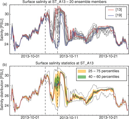
In Section 5, high internal variability was found in a number of different areas, in particular in Skagerrak. In the present section, a single event is examined in order to exemplify the impacts of the previous findings. The analyses in the present section are based on numerical results from September 26 to October 26 at position ‘Å13’, see Fig. 1. This time period and location was chosen to demonstrate the ensemble variations during an event with large differences between the ensemble members. In this particular case, large variability develops in an area with large horizontal salinity gradients due to the north-bound Baltic Current, which due to the Coriolis force, follows the Swedish coast. In the time leading up to the event, no especially large freshwater fluxes have been observed. Meteorologically, the period is dominated by relatively low winds and relatively stable pressure. On September 21 and 22, that is, 2 weeks before the event, a passing low-pressure system leads to moderate westerly winds slightly larger than 10 m/s for a few days, but no unusually strong winds seem to have triggered this particular event. As can be seen from Fig. 13a, the salinity variation is very small – less than 0.1 PSU RANGE – at the start and the end of the chosen period. However, between these dates, there are very large variations within the ensemble. For example, for October 07 member #19 predicts a decrease of about 1.7 PSU, from 24.9 to 23.2 PSU, while member #13 predicts an increase of about 5.4 PSU, from 25.8 to 31.2 PSU. The maximum ensemble RANGE in the period is about 8 PSU and occurs on October 8 (the equivalent maximum value of σ _SS is about 3 PSU). Two days later, the RANGE is <0.5 PSU, decreasing to <0.1 PSU after further a few weeks. Therefore, the variability, computed as RANGE in this case, varies about two orders of magnitude within the examined period. It is important to note that for a particular point in time and space, for example, Å13 at 2013-10-07 19:00 UTC, the distribution of salinity values from the ensemble members is very uneven and does not at all resemble a uniform or Gaussian distribution. The salinity varies between 23.5 and 31.3 PSU; several members predict values very close to the minimum, while none predicts salinity within the 24–26 PSU interval. Around the time of maximum RANGE, the ratio of RANGE to STDDEV shows significant variation (results not shown) with a minimum ratio of 2.5 around the time of maximum RANGE, and subsequently increasing rapidly to 4.9. If these numbers are compared to the computed percentiles found for a Gaussian distribution, see Section 2, then it seems unlikely that the distribution could be Gaussian. Time series of computed statistical variables is shown in Fig. 13b. It is interesting that the 25–75 percentile range shown in yellow often, for example, 2013-10-08, covers a very large part of the total range, as this indicates that 50% of the simulations are at the extreme ends of the interval. At other times, the 25–75 percentile band is very narrow, which could indicate a common tendency around the median with fewer outliers near the extremes. It should also be noted that there is often a significant difference between the median and mean values. On several occasions, the mean value does not even fall within the 40–60 percentile range shown in green. It is important to keep in mind the uneven/unpredictable distribution, if the ensemble is used to deduce more general features of the model stochastics.

Fig. 13 Time series of surface salinity at position ‘Å13’ in eastern Skagerrak from September 26 to October 26. Surface salinity of the 20 ensemble members, highlighting two particular members (a), and time series of statistical properties (b) including minimum and maximum values (grey), median (blue) and mean (red) values, and two percentile intervals. Dashed black lines indicate times used in later figures: 2013-10-04 20:00 and 2013-10-08 00:00.

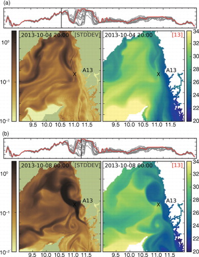
If the surface salinity in Skagerrak – near the Å13 position – is examined in detail, then it becomes apparent that the high internal variability at Å13 during this event may be caused by uncertainty in the positions of eddies and fronts in the area. In Fig. 14, the surface salinity in Skagerrak is depicted for two particular dates. Data for a single ensemble member are compared to ensemble variability σ _SS. The dates correspond to, respectively, very low and very high ensemble variability at Å13. On 2013-10-04 20:00, the ensemble members predicted nearly the same salinity value at Å13. At this time, there are high values of σ _SS north of Å13 and near the Norwegian coastline, but not closer to Å13, where the value is σ _SS=0.2 PSU, see Fig. 14a, left panel. The surface salinity for member #13 shows that there is a front off the coastline that separates the low saline waters along the coast line and the high saline waters in the centre of Skagerrak, see Fig. 14a, right panel. Obviously, the surface salinity distribution for the other ensemble members is similar to member #13, except for locations with high σ _SS. On 2013-10-08 00:00, the ensemble members predict very different surface salinity at Å13, see Fig. 13. The standard deviation is now above 2.0 PSU over a large area in eastern Skagerrak (Fig. 14b, left panel), as the ensemble members disagree on the exact locations of a front and eddy in the area. The online material includes animations of surface salinity, both in the form of frames like Fig. 14, and for two particular ensemble members (#13 and #19) side by side. Such animations provide valuable insights into the workings of internal variability.

Fig. 14 Surface salinity in eastern Skagerrak on 2013-10-04 20:00 (a) and 2013-10-08 00:00 (b), where X indicates the location for position ‘Å13’. Sea surface salinity STDDEV (PSU) (left) and surface salinity (PSU) for ensemble member #13 (right). In each subfigure, the top panel indicates time in a way consistent with Fig. 13.

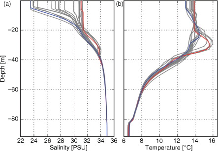
The different pathways for the water masses in the ensemble members can also be observed deeper in the water column. On October 8, the mixed layer depth in the different ensemble members varies from 3.5 to 20 m, and the salinity RANGE at 20 m depth is 1.8 PSU, see Fig. 15a. The vertical variations in temperature are also significant on this occasion, where some members predict temperature increase of almost 2 °C from 20 to 30 m depth, while other members predict a decrease from the mixed layer towards the bottom, see Fig. 15b.

Fig. 15 Vertical profiles of salinity (a) and temperature (b) for individual ensemble members on 2013-10-08 at position ‘Å13’. Members #13 (red) and #19 (blue) are highlighted identical to Fig. 13a.

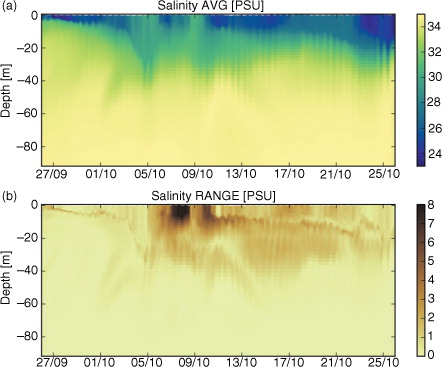
The temporal evolution of salinity average and range is shown in Fig. 16. The previously observed high variability periods, see Fig. 13, can be refound in Fig. 16b. The highest salinity variability is found at and just below the free surface. If the variability is compared with the ensemble average in Fig. 16a, then it is noted that the maximum salinity variability occurs right after a period with well-mixed conditions, where there is very little salinity difference in the upper half of the water column. The present single event does not, however, seem to be enough to conclude if there is a firm connection between well-mixed conditions and high variability. The temperature average and range at Å13 for the same period are depicted in Fig. 17. From Fig. 17a, it is noted that both before and after the well-mixed period, there are periods with warmer waters at intermediate water depths. This is interpreted as ‘warm summer waters’, less affected by the autumn cooling of the surface. Compared with the surface salinity, the surface temperature has very little ensemble variability. This is likely because the surface temperature is tightly bound to the used meteorological forcing, which does not vary between the ensemble members. Further, it is clear from Fig. 17b that large temperature variability may be found in the intermediate waters. Thus, high variability in temperature and salinity may be quite unrelated phenomena.

Fig. 16 Time-depth plot of salinity AVERAGE (a) and RANGE (b) over the ensemble at position ‘Å13’.

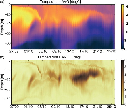
Fig. 17 Time-depth plot of temperature AVERAGE (a) and RANGE (b) over the ensemble at position ‘Å13’.

7. Conclusions and further work

The stochastic uncertainty connected to the simulations of a single 3-D baroclinic ocean model setup has been examined, namely the FCOO NS1C operational setup, see Büchmann et al. (2011). The model compilation and execution are fully repeatable, so the uncertainty is unrelated to random rounding effects taking place in the floating point computations. Rather, the stochastic features are attributed to cascading effects from small-scale to larger mesoscale features. Perturbations have been made solely on the salinity initial conditions, and it has been shown that even the slightest perturbations, corresponding to well under 1 µg salt, result in simulation branching and in large local differences of several PSUs within a few days of simulation.

To estimate the stochastic component inherent to a single numerical experiment, a 20-member ensemble based on initial perturbations of 10⁻¹² PSU has been created and run for 1 yr. No perturbations have been made to the equations of state or the forcing fields driving the simulations. During an initial phase, the ensemble variability grows exponentially fast with as much as seven orders of magnitude in a single day. It is concluded that the growth is due to two inherently different processes. Primarily, a simple repetition of the time-stepping computations causes the original slight differences to increase exponentially in time. This happens even if all ensemble members go over exactly the same numerical instructions sequence. Secondarily, however, discrepancies in the number of repetitions in an iterative procedure for vertical stability causes ‘sporadic jumps’, as some ensemble members may make additional computations.

It was found that the ensemble variability depends heavily on the area. For instance, the average sea-surface salinity ensemble standard variation varies about a factor of 20 from the German Bight to Skagerrak, with the highest values in Skagerrak. High ensemble variability was found in areas with high mesoscale activity, such as Skagerrak and Kattegat, where eddies may propagate reasonably unrestricted by coastal processes. However, also some areas with many fronts, such as the Sound, show relatively high ensemble variability. It has been shown that in some cases the maximal ensemble variability may be found not at the surface or bottom, but in the interior of the water column, such as near a bottom boundary layer developing under a freshwater outflow. In the Baltic Sea, there are also regions with high mesoscale activity, but the spatial salinity gradients are sufficiently small to limit the variability. In general, high internal model variability does not seem to be initiated by extraordinary forcing, such as storms or very large freshwater outflow.

Periods with very high ensemble variability have been found to be short-term events and very limited spatially. The impact from these events on the annual statistics is relatively limited. For example, the found annually averaged surface salinity ensemble standard deviation is about an order of magnitude smaller (0.1 PSU vs. 3–4 PSU for Kattegat and Skagerrak) compared wih the results by an MME study (Golbeck et al., 2015), that is, an intra-model study. There are several reasons for the much higher intramodel variability values, such as different model resolutions and different forcings, including the freshwater fluxes. However, the high internal variability events increase the uncertainty connected to setup tuning and validation.

The stochastic distribution of, for example, salinity within the ensemble – found in the present work – is itself variable not just in magnitude. Sometimes, the ensemble values are concentrated around a common average with a few outliers, while other periods show a ‘bundling’ of values at opposite ends of an interval with very few members predicting intermediate results. Results indicate that the model ensemble probably does not follow a normal distribution. This may bear an impact on data assimilation where it is often an assumption that model errors follow a particular ensemble distribution. The time scales for the model internal variability to reach a final saturated state also exhibit significant variations between regions – for the surface variables from in the order of 5 d in the Great Belt to around 2 months for the Bornholm Basin. For the bottom variables, the time scales tend to be larger, and for the bottom temperature in Kattegat, the time scale was found to be too large to be estimated by the present 1-yr simulation. The estimated time scales seem consistent with the findings by Fu et al. (2011), who report that the effects of data assimilation in the transition area can ‘persist for nearly 3 weeks’, while Losa et al. (2012) reported a much shorter time scale of ‘up to 5 days’ in the North Sea with SST assimilation.

For an event with very high ensemble variability of surface salinity at a particular position in Skagerrak, it has been observed that there was not an equivalent high variability of surface temperature. Further, very high temperature variability was found – only in the middle of the water column. This variability may be decoupled from the surface mesoscale structures. As a consequence, it may be difficult to decrease the variability in the deeper layers of the waters, if data assimilation of surface quantities only is considered. However, the actual SST values may be useful if remote sensing of SST is used in recursive selection and re-branching of ensemble members, as described by van Leeuwen (2010). Then, data for each ensemble member are compared to observations, and the best-fitting members are selected for further processing and re-branching, while badly fitting members are discarded and exempted from further simulation. It may be successful in areas, where the time scale for temperature variability is sufficiently large and there is enough ‘open water’ for the SST to actually produce a picture of high enough resolution without coast effects. Thus, candidates, where such ideas may prove successful, are areas which have both relatively large geographic extend and a large time scale of SST ensemble variability. In particular, the Bornholm and the Arkona Basins seem candidates for this application, as the time scales of the SST ensemble variability development seem very large (40–70 d). In Skagerrak and Kattegat, the estimated time scales to full decoupling of the ensemble members are smaller – in the order of a few weeks (17–19 d). Thus, it is expected that the selection and re-creation process might be repeated at least several times per week in order to keep the ensemble members reasonably close to the observations. However, if an operational ocean forecast model is to be significantly improved by reducing the internal variability and bringing the simulated mesoscale features ‘in phase with nature’, it may require additional data sources such as altimeter, RF arrays, ferry-boxes and on-line buoys and observation stations. In fact, many operational models for the North Sea–Baltic Sea assimilate satellite-derived SST or in-situ data, including ferry-box data, see Golbeck et al. (2015). However, in operational modelling assimilation, combining the full variety of measured data seems less used – if at all.

8. Acknowledgements

We would like to thank our colleagues at FCOO for good discussions, constructive criticism and liberal feedback. Also, we acknowledge our colleagues at BSH, DMI and SMHI for the data provided for the FCOO operational setup – data which have also been used for the present study. The reviewers are thanked for comments and suggestions, which have led to improvements of the manuscript.

Notes

¹For a 20-sample draw from a Gaussian (normal) distribution, the ratio RANGE/STDDEV has an average/expected value of 3.8 with a standard deviation of 0.40. Using Monte Carlo simulations, we find the equivalent 0.1%, 1%, 99% and 99.9% percentiles to be, respectively, 2.8, 3.0, 4.8 and 5.1.

²An animation of the initial development of the surface and bottom salinity standard deviation in the Danish waters is presented as part of the online material: dk.salt-std.surfbott-15min.avi.

³This event is presented as animation in online material as gbight.salt-std.surfbott-15min-jump.avi.

⁴Repeat until convergence.

⁵A figure including surface salinity data for all 20 members is available as part of the online material: dk.salt-data.surface.20130301.png.

⁶A figure including surface salinity anomalies for all 20 members is available as part of the online material: dk.salt-anomaly.surface.20130301.png.

⁷A13-area.salt.surface.dstd-dl3.avi.

⁸A13-area.salt.surface.d19-d13.avi.

References

- Brankart J. M., Candille G., Garnier F., Calone C., Melet A., co-authors. A generic approach to explicit simulation of uncertainty in the NEMO ocean model. Geosci. Model Dev. 2015; 8: 1285–1297. http://dx.doi.org/10.5194/gmd-8-1285-2015.
- Broström G., Carrasco A., Hole L. R., Dick S., Janssen F., co-authors. Usefulness of high resolution coastal models for operational oil spill forecast: the full city accident. Ocean Sci. 2011; 7(6): 805–820. http://dx.doi.org/10.5194/os-7-805-2011.
- Büchmann B., Hansen C., Söderkvist J. Improvement of hydrodynamic forecasting of Danish waters: impact of low-frequency North Atlantic barotropic variations. Ocean Dynam. 2011; 61: 1611–1617. http://dx.doi.org/10.1007/s10236-011-0451-2.
- Burchard H., Bolding K. GETM A General Estuarine Transport Model. Scientific Documentation. 2002. Technical Report EUR 20253 EN. European Commission, Ispra (VA), Italy. Online at: http://bookshop.europa.eu/en/getm-a-general-estuarine-transport-model-pbEUNA20253/.
- Chu P. C., Miller S. E., Hansen J. A. Fuel-saving ship route using the Navy's ensemble meteorological and oceanic forecasts. J. Def. Model Simulation Appl. Methodol. Technol. 2015; 12(1): 41–56. http://dx.doi.org/10.1177/1548512913516552.
- COAS. OSU Tidal Data Inversion. 2015. Online at: http://volkov.oce.orst.edu/tides/.
- Egbert G. D., Erofeeva S. Y. Efficient inverse modeling of barotropic ocean tides. J. Atmos. Ocean. Technol. 2002; 19(2): 183–204. http://dx.doi.org/10.1175/1520-0426(2002)019<0183:EIMOBO>2.0.CO;2.
- Fu W., She J., Zhuang S. Application of an ensemble optimal interpolation in a North/Baltic Sea model: assimilating temperature and salinity profiles. Ocean Model. 2011; 40(3–4): 227–245. http://dx.doi.org/10.1016/j.ocemod.2011.09.004.
- Golbeck I., Li X., Janssen F., Brüning T., Nielsen J. W., co-authors. Uncertainty estimation for operational ocean forecast products – a multi-model ensemble for the North Sea and the Baltic Sea. Ocean Dynam. 2015; 65(12): 1603–1631. http://dx.doi.org/10.1007/s10236-015-0897-8.
- Gustafsson B. High frequency variability of the surface layers in the Skagerrak during SKAGEX. Cont. Shelf Res. 1999; 19(8): 1021–1047. http://dx.doi.org/10.1016/S0278-4343(99)00008-4.
- Holt T. R., Cummings J. A., Bishop C. H., Doyle J. D., Hong X., co-authors. Development and testing of a coupled ocean atmosphere mesoscale ensemble prediction system. Ocean Dynam. 2011; 61(11): 1937–1954. http://dx.doi.org/10.1007/s10236-011-0449-9.
- Holtermann P. L., Burchard H., Gräwe U., Klingbeil K., Umlauf L. Deep-water dynamics and boundary mixing in a nontidal stratified basin: a modeling study of the Baltic Sea. J. Geophys. Res. Oceans. 2014; 119(2): 1465–1487. http://dx.doi.org/10.1002/2013JC009483.
- Lamb H . Hydrodynamics. 1932; 6th ed, Cambridge, UK: Cambridge University Press.
- Lindström G., Johansson B., Persson M., Gardelin M., Bergström S. Development and test of the distributed HBV-96 hydrological model. J. Hydrol. 1997; 201: 272–288. http://dx.doi.org/10.1016/S0022-1694(97)00041-3.
- Lorenz E. N. Deterministic nonperiodic flow. J. Atmos. Sci. 1963; 20: 130–141. http://dx.doi.org/10.1175/1520-0469(1963)020<0130:DNF>2.0.CO;2.
- Losa S. N., Danilov S., Schröter J., Nerger L., Maßmann S., co-authors. Assimilating NOAA SST data into the BSH operational circulation model for the North and Baltic Seas: inference about the data. J. Marine Syst. 2012; 122: 105–108. http://dx.doi.org/10.1016/j.jmarsys.2012.07.008.
- Melsom A. Mesoscale activity in the North Sea as seen in ensemble simulations. Ocean Dynam. 2005; 55(3): 338–350. http://dx.doi.org/10.1007/s10236-005-0016-3.
- Melsom A., Counillon F., LaCasce J. H., Bertino L. Forecasting search areas using ensemble ocean circulation modeling. Ocean Dynam. 2012; 62(8): 1245–1257. http://dx.doi.org/10.1007/s10236-012-0561-5.
- Molteni F., Buizza R., Palmer T. N., Petroliagis T. The ECMWF ensemble prediction system: methodology and validation. Q. J. Roy. Meteorol. Soc. 1996; 122(529): 73–119. http://dx.doi.org/10.1002/qj.49712252905.
- Nielsen M. H. The baroclinic surface currents in the Kattegat. J. Marine Syst. 2005; 55: 97–121. http://dx.doi.org/10.1016/j.jmarsys.2004.08.004.
- O'Dea E. J., Arnold A. K., Edwards K. P., Furner R., Hyder P., co-authors. An operational ocean forecast system incorporating NEMO and SST data assimilation for the tidally driven European North-West shelf. J. Oper. Oceanogr. 2012; 5(1): 3–17. http://dx.doi.org/10.1080/1755876X.2012.11020128.
- Oke P. R., Brassington G. B., Griffin D. A., Schiller A. The Bluelink ocean data assimilation system (BODAS). Ocean Model. 2008; 21(1–2): 3301–3311. http://dx.doi.org/10.1016/j.ocemod.2007.11.002.
- Sakov P., Counillon F., Bertino L., Lisæter K. A., Oke P. R., co-authors. TOPAZ4: an ocean-sea ice data assimilation system for the North Atlantic and Arctic. Ocean Sci. 2012; 8(4): 633–656. http://dx.doi.org/10.5194/os-8-633-2012.
- Shchepetkin A. F., McWilliams J. C. The regional oceanic modeling system (ROMS): a split-explicit, free-surface, topography-following-coordinate oceanic model. Ocean Model. 2005; 9(4): 347–404. DOI: http://dx.doi.org/10.1016/j.ocemod.2004.08.002.
- Toth Z., Kalnay E. Ensemble forecasting at NMC: the generation of perturbations. Bull. Am. Meteorol. Soc. 1993; 74(12): 2317–2330. http://dx.doi.org/10.1175/1520-0477(1993)074<2317:EFANTG>2.0.CO;2.
- Umlauf L., Burchard H. Second-order turbulence closure models for geophysical boundary layers. A review of recent work. Cont. Shelf Res. 2005; 25: 795–827. http://dx.doi.org/10.1016/j.csr.2004.08.004.
- Undén P., Rontu L., Järvinen H., Lynch P., Calvo J., co-authors. HIRLAM-5 scientific documentation. 2002. Online at: http://hirlam.org/index.php/hirlam-documentation.
- van Leeuwen P. J. Nonlinear data assimilation in geosciences: an extremely efficient particle filter. Q. J. Roy. Meteorol. Soc. 2010; 136: 1991–1999. http://dx.doi.org/10.1002/qj.699.