To what extent is your data assimilation scheme designed to find the posterior mean, the posterior mode or something else?

Abstract

Recently there has been a surge in interest in coupling ensemble-based data assimilation methods with variational methods (commonly referred to as 4DVar). Here we discuss a number of important differences between ensemble-based and variational methods that ought to be considered when attempting to fuse these methods. We note that the Best Linear Unbiased Estimate (BLUE) of the posterior mean over a data assimilation window can only be delivered by data assimilation schemes that utilise the 4-dimensional (4D) forecast covariance of a prior distribution of non-linear forecasts across the data assimilation window. An ensemble Kalman smoother (EnKS) may be viewed as a BLUE approximating data assimilation scheme. In contrast, we use the dual form of 4DVar to show that the most likely non-linear trajectory corresponding to the posterior mode across a data assimilation window can only be delivered by data assimilation schemes that create counterparts of the 4D prior forecast covariance using a tangent linear model. Since 4DVar schemes have the required structural framework to identify posterior modes, in contrast to the EnKS, they may be viewed as mode approximating data assimilation schemes. Hence, when aspects of the EnKS and 4DVar data assimilation schemes are blended together in a hybrid, one would like to be able to understand how such changes would affect the mode- or mean-finding abilities of the data assimilation schemes. This article helps build such understanding using a series of simple examples. We argue that this understanding has important implications to both the interpretation of the hybrid state estimates and to their design.

• data assimilation
• ensemble methods
• variational methods

1. Introduction

Our main goal in this work is to link the methods of variational data assimilation to the typical approach taken in ensemble data assimilation. Ensemble data assimilation is built upon the statistical framework of Bayesian methods and, therefore, views the data assimilation problem as centred around the determination of a probability density function (PDF) describing the uncertainty in the state. While many contemporary derivations on variational methods also derive these methods from a Bayesian framework (e.g. Bennett, 2002; Tarantola, 2005; Lewis et al., 2006), much of the early work on variational methods in meteorology were less clear about its connection to PDFs and Bayesian methods (e.g. Talagrand and Courtier, 1987; Gauthier, 1992; Courtier et al., 1994). We begin here by reviewing different approaches to state estimation from a statistical point of view and then relating them to the problems to be addressed here.

One approach to state estimation is to try and find the minimum error variance estimate (or mean of the posterior distribution) of the state given a prior distribution of possible true states and new observations. This approach is concordant with ensemble forecasting because the mean of the initialised ensemble is generally set equal to the state estimate. Ensemble Kalman filters (EnKF) and smoothers (EnKS) both fall into this category. In these algorithms, the posterior mean is approximated as a linear function of the new observations and can be expressed in terms of a first guess (prior mean) plus a correction term that depends on, among other things, the covariance of a prior ensemble of non-linear forecasts. This state estimation procedure will be referred to as the Best Linear Unbiased Estimate (BLUE) throughout this manuscript. The terms ‘smoother’ and ‘filter’ (e.g. Jazwinski, 1970; Li and Navon, 2001) distinguish a difference between the time the observations are taken and the time at which the analysis is made. In a filter, one finds the state estimate at a particular time using observations that were taken at the analysis time, whereas, with a smoother, one can also use observations taken at times distinct from the analysis time. Because the observations used in a smoother are distributed through time the forecast error covariance matrix is 4-dimensional (4D) (i.e. varies in both space and time) and describes the covariance of the error in variables that are separated through this 4D space-time. The fully non-linear model is required to create this forecast error covariance matrix from knowledge of the posterior distribution at the previous assimilation step.

Another approach to state estimation is to find the minimum of some relevant penalty function. Many variational data assimilation schemes fall into this category (e.g. Talagrand and Courtier, 1987; Navon et al., 1992; Klinker et al., 2000; Mahfouf and Rabier, 2000; Rabier et al., 2000; Rabier, 2005; Rawlins et al. 2007; Zhang et al., 2014). This penalty function is connected to the minimum variance approach as it is (up to an additive constant) the negative logarithm of the product of the prior and observation likelihood PDFs and hence, by Bayes’ theorem, the state that minimises this penalty function is the most likely state, or mode of the posterior PDF. The minimum of the penalty function occurs where its gradient is zero, which implies that it may be found by means of a minimisation method (e.g. Incremental/Gauss–Newton) that employs an ‘outer loop’ in which one iteratively computes the gradient of the penalty function around the latest guess of the mode, then uses this gradient to make better guesses, and so on.

Variational methods are currently well established at operational forecasting centres. Their use of an (approximate) tangent linear model (TLM) and its adjoint obviate the need for the specification of the 4D forecast error covariance matrix. However, variational methods do require the specification of an initial time 3D forecast error covariance matrix. This initial time covariance matrix should change from one data assimilation cycle to the next due to changes in meteorological conditions and also to changes in the observational network. Ensemble methods are constructed such that they can produce an estimate of this time varying covariance matrix. However, historically, variational methods employed a fixed ‘climatological’ model of this covariance matrix. Recent work has attempted to make use of the ensemble's estimate of this initial time covariance matrix in a hybrid formulation. This hybrid variational framework employs an initial time error covariance matrix that is a weighted average of a climatological error covariance matrix and an ensemble covariance matrix (Buehner et al., 2009, 2013; Clayton et al., 2013; Kuhl et al., 2013; Lorenc et al., 2015; Wang and Lei, 2014; Kleist and Ide, 2015).

If either the prior distribution or observation likelihood is non-Gaussian, the most likely state estimate (the posterior mode) will differ from the minimum error variance state estimate (the posterior mean). Without adjustments, comparison of the textbook descriptions of variational methods with outer loops (e.g. Bennet, 2002; Tarantola, 2005; Lewis et al, 2006) with actual operational implementations of variational schemes with outer loops (e.g. Rabier et al., 2000; Rosmond and Xu, 2006) make it clear that these operational implementations would find the mode of the posterior distribution if forecast and observation error covariance matrices were accurately specified and an accurate TLM were available. Lorenc and others (e.g. Lorenc 1986; Lorenc, 1997, 2003a 2003b; Courtier et al., 1994) have argued that the variational framework should be adjusted so that it achieves a state that is more like the posterior mean than the mode. Lorenc and Payne (2007) argue that the most likely state is less useful than the minimum error variance estimate when the time scale of predictability is shorter than the length of the data assimilation window. Also, for the sake of statistical consistency, it is more natural to centre ensembles of perturbations about the mean than it is to centre them about the mode. On the other hand, the time evolution of the ensemble mean state is not governed by the equations that are in our numerical models nor is the mean governed by the laws that govern the evolution of a single realisation of nature. The time evolution of the mode is approximated by our numerical weather prediction (NWP) models and hence, if ones primary interest is to assess the realism of NWP trajectories, one could argue that the mode is more useful than the mean. This manuscript does not attempt to take part in this discussion as to whether the posterior mode or posterior mean is best for state estimation. Rather, we will carefully discuss the relationships between mean-finding and mode-finding methods and how ensembles may be used in either method.

We will carefully compare posterior BLUE-finding algorithms to mode-finding algorithms. We recall that the standard mode-finding algorithms, referred to as the Gauss–Newton and incremental method (Courtier et al., 1994), can be written in a form very similar to the form of the equation we described earlier as a ‘smoother’ to find the BLUE estimate across an observation window in time. This formulation of the mode-finding problem has been referred to in the past as the ‘Dual’ form (Courtier, 1997; El Akkraoui et al., 2008). One purpose of this article is to point out that despite the superficial similarity between the posterior BLUE-finding algorithms and mode-finding algorithms that these two algorithms are fundamentally different whenever non-linearity is present in the system. We will argue that this has important ramifications to the recent work to fuse ensemble and variational 4D data assimilation methods by combining their covariance models. Furthermore, the tests required to check the accuracy of a data assimilation method to find the BLUE are substantially different from the tests required to check a method to find the mode. We believe that a clear understanding of these differences has intrinsic value and may ultimately improve operational data assimilation systems.

Furthermore, it is well known (Li and Navon, 2001; Lorenc, 2003b; Fairbairn et al., 2014) that when errors are small enough to be governed by linear dynamics and the prior and observation likelihood are Gaussian, then there is no need for an outer loop in 4DVar, and in this case the Kalman smoother and 4DVar have the same algebraic solution. We focus on the differences between 4DVar with an outer loop, the Kalman smoother and the ensemble Kalman smoother in the presence of non-linearity (either in the model or the observation operator). When a 4DVar algorithm is used in the presence of non-linearity but without application of the outer loop then the 4DVar algorithm can be thought of as a BLUE-estimating extended Kalman smoother because it is propagating the covariance matrix across the window using a linearised version of the forecast model (Courtier, 1997; Lorenc, 2003a). We emphasise that the extended Kalman smoother is not a mode-finding algorithm and therefore one cannot consider the 4DVar algorithm as a mode-finding algorithm when its goal is the same as the BLUE-estimating extended Kalman smoother. Therefore, throughout this article we will consider both EnKFs and 4DVar algorithms with no outer loop as BLUE-estimating methods and will compare and contrast them with mode-estimating methods.

The manuscript is organised as follows. In Section 2, we illustrate the basic model setup used throughout the text. In Section 3, we write down the equations for the minimum error variance estimate in the form of a ‘smoother’. In Section 4, we develop the strong-constraint form of the 4DVar problem and derive the incremental method for finding the posterior mode. In Section 5, we delve deeper into the properties of the TLM necessary to find the mode using an incremental method and compare this to a linearised model referred to as a statistical linear model. In Section 6, we compare and contrast methods for testing the quality of mode-finding and BLUE-finding methods. In Section 7, we close the manuscript with a brief summary and suggestions for the future development of data assimilation algorithms that attempt to blend aspects of ensemble and 4DVar methods.

2. Model

The analysis presented below will make use of a scalar physical system in order to illustrate the basic results in their simplest forms. Our emphasis is on the effects of non-linearity, not the difficulties that arise from a large state dimension, and this simple scalar example allows us to illustrate our main points most clearly.

We assume that the state of the physical system at the time t=0 is uncertain and this uncertainty is described by a prior distribution that is Gaussian with mean and variance . The reason for choosing this particular value for will be explained in detail in Section 5. We will further assume that we have an observation of the state at t=1 with a Gaussian observation likelihood with error variance, R=1 and take for our example observation y ₁=2.5.

The ordinary differential equation (ODE) governing the evolution of the variable of interest is1

where f(x) is some potentially non-linear function defining the tendencies of the model and the subscript on the state variable denotes its relevant time. We may integrate eq. (1) in time from t=0 to the time of the next observation at t=1 to define a non-linear mapping from t=0 to t=1:2

where the subscript on M ₁₀ denotes that this mapping propagates a state at t=0 to t=1. The mapping in eq. (2) is different for different lengths of time between observations and therefore the degree of non-linearity in eq. (2) changes with the time between observations. While the mapping [eq. (2)] changes as a function of the time to the next observation the underlying model [eq. (1)] is always the same.

For concreteness, we define the model in eq. (2) as3

where a₀=5. This example model equation in eq. (3) was chosen carefully to have one real root for each final state, x ₁, i.e. it was chosen to have a known inverse. If this is not the case, and eq. (3) has multiple real roots of x ₀ for some particular value of the final time state, x ₁, then the resulting posterior at t=0 will be multi-modal if an observation at t=1 is near to this particular final time state. Additionally, the model [eq. (3)] was carefully chosen such that the dominant action for small values of the state, x ₀, is growth and for larger values the dominant action is saturation. We will see later that this can result in excessive growth in the TLM in certain situations.

3. Ensemble-based methods for the BLUE

Our goal in this section is to illustrate the basic properties of the forecast error covariance matrix required to find the minimum error variance estimate of a linear estimator, which is the posterior mean in the Gaussian case. In this section, we wish to update the state at t=0 and t=1 based on the observation at t=1. In the next section, we will develop a mode-finding algorithm that will only update the state at t=0 given the observation at t=1. Because we are updating the state at a time distinct from the observation time the standard nomenclature for this state estimation technique is to refer to this method as a ‘smoother’.

The prior covariance matrix obtained by propagating the prior distribution forward in time under the dynamics of the non-linear model would be:4

where , P ₀₁=P ₁₀=, angle brackets are used to denote an expectation has been taken, and5

is the joint prior density with p(x ₀) being the density describing the uncertainty at t=0 and p(x ₁∣x ₀) is the transition density describing how the model propagates the state from t=0 to t=1.

The integral in eq. (4) is computationally infeasible to evaluate in high-dimensional problems; in practice this integral is approximated by employing an ensemble of non-linear model runs beginning from random draws from p(x ₀) and pushed through eq. (2). In eq. (4), an ensemble of 10⁷ members was run to estimate using sample statistics.

The covariance matrix [eq. (4)] delivers the minimum error variance estimate of a linear estimator (Jazwinski, 1970) when used in the following formula:6

where H=[0 1], y₁ is the observation at t=1, R is the observation error covariance matrix and a superscript of a denotes the ‘analysis’ and a superscript of f denotes the prior mean. The expected squared error from estimating the state as eq. (6) is given by the similarly well-known formula:

In the next section, it will prove of interest to note that the first row of eq. (6) may be written as

and the initial time posterior variance around this minimum error variance estimate of a linear estimator is

which with eq. (4) and R =1 implies that on average the error variance at time 0 will be reduced from 1 to 0.459 by assimilating an observation at t=1.

The point here is that the correct gain matrix in eq. (8) to find the minimum error variance of a linear estimator is constructed by propagating the prior distribution under the dynamics of the non-linear model across the assimilation window. We shall hereafter refer to the estimate [eqs. (6) and (8)] as the Best Linear Unbiased Estimate (BLUE). We emphasise here that the ‘L’ in BLUE refers to the fact that the estimate [eq. (8)] is a linear function of the observation, and not to using a linearised model or linearised observation operator.

4. A variational method for the posterior mode

Our goal in this section is to illustrate the properties of the standard solution technique to find the maximum likelihood (mode) estimate and then compare this to the BLUE.

4.1. The incremental approach

Because the prior and the likelihood are Gaussian the well-known cost function, whose minimum is the mode of the posterior distribution at t=0, is:

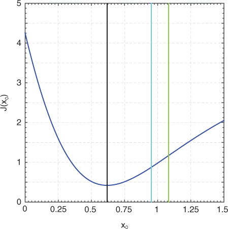
where R=1 is the observation error variance and we have made explicit that x ₁ is a function of x ₀. Equation (10) can be found in, for example, Rabier (2005). The cost function in eq. (10) for our example problem is plotted in Fig. 1.

Fig. 1 The cost function and important parameters. The blue curve is the cost function of eq. (4). vertical black line denotes the solution at the minimum of the cost function. Vertical cyan line denotes the true posterior mean. Vertical green line denotes the BLUE from the Kalman smoother in eq. (8).

Typically, this cost function is re-written in ‘incremental’ form through the definition of the perturbation, , where is referred to as the guess for the j ^th outer loop and whose form will become apparent in a moment. Using this perturbation, and linearising, allows the cost function [eq. (10)] to be written as an exactly quadratic problem of the form:

This cost function is then solved as a series of exactly quadratic problems of the form eq. (11) for fixed . Note that to obtain eq. (11) from eq. (10) we made an approximation in the observation weighting term. This approximation begins with a Taylor-series of the form

where13

is the TLM. To obtain eq. (11) from eq. (10), we use eq. (12) but neglect terms in the series that are quadratic and larger. In order for the quadratic term to be negligible, the following condition must be satisfied:

This condition implies that either or both:

Both conditions are identically the condition for a dynamical system whose evolution is nearly linear, where eq. (12) requires that the true model for the perturbations [eq. (3)] is at most weakly non-linear and eq. (16) requires that the perturbation is small. The question of whether these assumptions are ever satisfied in numerical weather prediction is a difficult one. If eq. (15) is satisfied, this implies that the TLM is largely independent of the state it is linearised around; this apparent lack of sensitivity to the state the TLM is linearised around is not seen in practice. This would seem to imply that the satisfaction of condition eq. (14) hinges on the smallness of the perturbation [eq. (16)]. Similarly, the perturbation, δx ^j , approaches zero when the sequence of quadratic problems in eq. (11) convergences to the mode.

If we take a derivative of eq. (11), set the result to zero, and solve we find:

where and

If we re-write eq. (17) by removing the various perturbation quantities, we find:

Equation (19) is identical to eq. (9.49) of Jazwinski (1970). Equation (19) is also identical to the solution procedure obtained from the Gauss–Newton method (see Appendix A), which implies that the solution to incremental 4D-Var is identical to the solution obtained through the Gauss–Newton method. Hence, if we desire for the incremental method to converge towards the minimum of the cost function we need eqs. (15) and (16) to be satisfied just as the Gauss–Newton method needs to neglect a specific term in the Hessian through the identical requirement that eqs. (15) and (16) be satisfied. We point out that if one replaces the exact TLM with an approximation in the Gauss–Newton method or in the incremental method the end result is the same; they converge to the same state, which is not the minimum of eq. (10).

Finally, if the incremental method is stopped after the first iteration then eq. (19) simply reduces to the extended Kalman Smoother (EKS), viz.

where we emphasise that the EKS differs from the BLUE in eq. (8) because the variances are propagated by the TLM rather than calculated from an ensemble of non-linear model runs.

4.2. Prior and posterior variances

The quantity in eq. (17), that we label as , is only equal to the posterior error variance when the model governing the dynamics is linear. When the dynamics are non-linear it is not equal to the posterior error variance. As an example, if we evaluate eq. (18) at the mode identified in Fig. 1 we find a ‘posterior error variance’ of 0.0593, which we compare to the posterior error variance of the BLUE, which is 0.459, and is obtained from eq. (9). The posterior error variance of the true posterior mean at t=0 is 0.240 and the variance about the mode must be larger than this because the variance about the posterior mean is the minimum variance estimate. Therefore this quantity in eq. (18) that is often referred to as a ‘posterior error variance’ is not actually a useful approximation to the posterior variance because of the non-linearity in the model.

As we will show below even though is not an accurate estimate of the error variance of the posterior it is precisely the correct quantity required for a mode-finding method to converge to the mode. Similarly, we show below that this has important ramifications to the fusing of ensemble and variational methods because the ensemble method must be able to deliver eq. (18), and not an accurate estimate of the posterior variance, if the algorithm is intended to converge to the posterior mode. Please see Appendix B for more discussion as to how the Hessian relates to the error variance about the mode. Additional discussion of the relationship between the implied ‘variances’ in 4DVar and the true variances is given in Section 5.

Equation (19) gives the appearance of the formula for the BLUE [eq. (8)], but with a modified innovation. We believe that this has helped spur interest in the desire to merge ensemble Kalman filtering methods with those of 4DVar. This however immediately leads to the following question: is the ‘gain’ required in eq. (19) to obtain the mode the same object that is required to find the BLUE using eq. (8)? If not, then the merging of ensemble and 4DVar methods must be done very carefully if one wants the mode from a hybridised version of 4DVar that makes use of an ensemble covariance matrix. We answer this question next.

The implied ‘Kalman gain’ for eq. (19) is

We may compare this gain to the gain in eq. (8)

These two gains will be the same if it is true that P ₀₀ M ₁₀=P ₀₁ and M ₀₁ P ₀₀ M ₁₀=P ₁₁, which implies that we assume that eq. (4) is equal to

where we have evaluated this matrix for our example problem and linearised the TLM around the mode. This apparent desire to swap the TLM's propagation of the initial time covariance matrix for the ensemble's propagation of this matrix is motivated by the urge to develop algorithms that can do what TLM's do without the typical expense in development and maintenance efforts of the TLM. This swapping of the TLM's estimate of the 4D covariance matrix for the ensemble's version has recently been referred to as ‘4DEnVar’ (Lorenc et al., 2015).

The mode-finding gain [eq. (21)] is a non-linear function of the reference state because the TLM, M ₁₀, is a function of the reference state that it was linearised around. In contrast, the gain in eq. (22) is a constant. Clearly, they cannot be the same. Let's create a specific example to illustrate the difference between eqs. (21) and (22). The gain in eq. (21) is most sensibly evaluated at convergence, which means evaluated at the mode. This implies that the mode-finding gain [eq. (21)] depends on the observation (because the mode depends on the observation) while the BLUE-finding gain [eq. (22)] is strictly independent of the observation. We iterate eq. (19) to obtain the mode such that G _mode =0.236 and G _mode =0.347. Hence, we have now shown that the correct gain matrix for the BLUE is not the one required to find the maximal likelihood estimate using an incremental method. This immediately implies that swapping the covariance matrix in a 4D-Var scheme with an outer loop for that of an ensemble-derived covariance matrix will no longer find the mode. Note however that replacing the covariance matrix in a 4D-Var scheme without an outer loop for that of an ensemble-derived covariance matrix may lead to a better estimate of the BLUE.

5. Tangent and statistical linear models

The use of ensemble methods in 4DVar algorithms has led to the desire to use hybrid ensemble/static covariance matrices in the algorithm. One idea for a ‘hybrid’ 4DVar algorithm is to make use of the ensemble covariances through time rather than to use a TLM. There are at least two ways that have been discussed in the literature as to how one might go about this. First, one can compare the prior covariance matrix from the TLM [eq. (23)] to the prior covariance matrix in eq. (4) and conclude that one could simply swap the prior covariance matrix from the TLM [eq. (23)] for the prior covariance matrix in eq. (4). We have already shown in Section 4 that this will not deliver the mode when used in the incremental method. It will however deliver the BLUE when an outer loop is not invoked, and this practice is useful for BLUE-finding algorithms. Second, one could keep the prior covariance matrix from the TLM [eq. (23)] as it is, but replace the TLM with a statistical approximation based on the covariances from the prior ensemble. This section will discuss the implications of this second approximation.

5.1. Tangent linear model

We begin with the TLM. The TLM, M ₁₀, used to find the mode is defined in eq. (13) and is to be understood in the sense of a Taylor-series about a model state, , viz.

Clearly, the TLM [] in eq. (24) provides an excellent approximation to the state x ₁ when the conditions in eqs. (15) and (16) are satisfied. This is the standard ‘linear’ result in which the size of the initial perturbation defines the quality of the TLM's propagation of a potentially non-linear perturbation evolution. This property that a TLM does not perfectly propagate a non-linear perturbation has been discussed numerous times in the meteorological literature (e.g. Errico et al., 1993; Errico and Raeder, 1999; Lorenc and Payne, 2007). Nevertheless, the TLM, whether it propagates a non-linear perturbation correctly or not, is still the object that delivers the correct gradient for the descent required to minimise eq. (10). If one is not interested in minimising eq. (10), but is in fact interested in obtaining a solution like the BLUE, then the use of a linear model that more accurately propagates a non-linear perturbation may be advantageous. This type of linear model is discussed in the next section.

The TLM has the computationally useful property that successive operations of the TLM can be thought of as propagating a perturbation through time (Le Dimet and Talagrand, 1986; Courtier, 1997). We can see this by defining the additional non-linear mapping that propagates from t=1 to t=2, viz.

Note that the TLM from t=0 to t=2 can therefore be written as

which explicitly makes use of the ‘linearity’ of the chain rule. One of the things we will show in the next section is that a statistical linear model does not have this property because it is not actually a gradient of the model and therefore the chain rule does not give it the property [eq. (26)].

5.2. Statistical linear models

One of the main advantages obtained from using a linear model that more accurately predicts the non-linear evolution of a perturbation than a TLM is that its variance estimates are more like that of an ensemble of non-linear model runs. This linear model that more accurately propagates variances than a TLM will be referred to here as a statistical linear model (SLM).

The SLM is the best unbiased linear model (in a least square sense) between t=0 and t=1. Hence, we make the assumption that the mean of the transition density, p(x ₁∣x ₀), is a linear function of x ₀, viz.

and subsequently search for the that minimises the variance, viz.

This is the standard procedure to determine the regression model in eq. (27) that minimises the distance between x ₁(x ₀) and in the sense of mean-square. The solution is

where

Equation (29) is consistent with Lorenc and Payne (2007) and Payne (2013); our eq. (29) has been generalised though by defining eq. (28) with respect to the joint prior density while Lorenc and Payne (2007) and Payne (2013) defined their SLM with respect to a centred version of the prior, i.e. . Their assumption is well justified for strong constraint, but for weak-constraint, when the transition density, p(x ₁∣x ₀), has non-zero variance and a possibly complex structure, the SLM must be defined against the joint prior density as is done in eq. (28).

Equation (29) shows that , which implies that is typically a better estimate of the state x ₁ obtained by initialising the non-linear model with the specific initial time value x ₀ than the prior mean , which is not conditioned on any particular state. Note that while the TLM is linearised around some specific state, the SLM is more properly thought of as calculated for some particular distribution with variance, P ₀₀. This implies that the SLM must be recalculated for every prior distribution much like the TLM must be linearised around different reference states.

The SLM in eq. (29) is related to the TLM [eq. (13)] in the following way. Because we will need to apply an expectation operator to eq. (24) we technically must assume that the support for p(x ₀) is entirely contained within the radius of convergence for the Taylor-series in eq. (24). With this assumption, we may apply an expectation operator to eq. (24) to obtain an equation for the mean

Here we see that the mean of the marginal prior does not follow a trajectory of the non-linear model. This is shown explicitly by eq. (31) whose difference from a trajectory is in fact forced by the variance of the perturbations, much like the forcing of the mean flow from eddies in wave-mean flow interaction theory (e.g. Pedlosky, 1987).

We may subtract eq. (31) from eq. (24) to obtain

where . We might multiply eq. (32) by , apply the expectation operator, and divide by P ₀₀ to obtain

where T ₀₀ is the third moment of the prior and F ₀₀ is the fourth moment of the prior. Equation (33) reveals the conditions when this SLM differs from a TLM. Equation (33) shows that the SLM is the explicit TLM plus information from higher order moments of the prior. These terms reveal that asymmetry and long tails of p(x ₀) are required for the explicit TLM and the SLM to differ significantly. Another way the SLM may differ from the explicit TLM is when the model is strongly non-linear such that the derivatives of the TLM with respect to the state are large. Conversely, eq. (33) shows that an SLM can be made into a TLM if the SLM is derived in eq. (28) by using a ‘prior’ distribution that is symmetric (such that odd moments vanish) and has infinitesimal variance (such that the even moments are infinitesimal). An example of an SLM designed to mimic the TLM is presented in an idealised model setting in Sakov et al. (2012) and Bocquet and Sakov (2014). The use of perturbations with infinitesimal variance has been suggested to be quite difficult in real-world numerical weather prediction where the non-linear model describes important physical processes using ‘if-switches’ (Lorenc and Payne 2007).

We showed above that the TLM has the computationally useful property that successive operations of the TLM can be thought of as propagating a perturbation through time. Here, we test this property for SLMs. First, note that we may reproduce the expansion in eq. (33) but for the SLM that propagates from t=0 to t=2 as

If it were true that the SLM had the property described by eq. (26), then eq. (34) would be equal to

Subtracting eq. (35) from eq. (34) reveals at leading order the following term:

Because one cannot accurately propagate the third moment using the TLM the difference in brackets does not vanish. Similarly, the higher order terms in the expansion can each be shown to suffer the same issue and therefore eq. (36) does not vanish.

This result has important ramifications to the suggestion to replace the TLM and adjoint in 4D-Var with localised ensemble-based SLMs. Specifically, the result [eq. (36)] shows that using such SLMs in a chain rule [eqs. (12) and (13)] will not result in the SLM over many time steps. Because this property is computationally important to the timely solution of the 4DVar problem the Perturbation Forecast (PF) model approach has been suggested (e.g. Lorenc, 1997; Lorenc and Payne, 2007). In the PF model approach, the non-linear governing equations are linearised, but then tuned for finite-amplitude perturbations. In this case, if one wanted to best approximate a SLM one would need to tune this PF model to minimise37

where n is the number of discrete times defining the data assimilation time window of interest; the covariance matrices pertain to the prior density and is a PF model that is applied in the sense of eq. (26). Note that this differs from the way to tune a SLM across the same time window:38

where the are separate matrices each tuned to best deliver the covariance between time i and 0 of the prior. For both schemes, if one were to change the length of the time window or the amplitude of the prior variances one would need to retune the PF model. Nevertheless, this PF model approach makes the explicit assumption that the property [eq. (26)] holds and therefore can never precisely equal the performance of an SLM because SLM's do not have this property.

An obvious third approach is to simply localise 4D ensemble covariances (Bishop and Hodyss, 2011; Lorenc et al., 2015). This approach entirely circumvents the need for a TLM and adjoint and arguably is the most promising means of using a 4D-Var framework to obtain an approximation to the BLUE. As noted in Bishop and Hodyss (2011), some form of adaptive localisation may significantly enhance the accuracy of this approach.

5.3. Numerical example

We provide an example of these differences between the TLM and SLM using our example problem of Section 2. We linearise the TLM around a variety of reference states and plot the value of the TLM (our TLM is a scalar) in Fig. 2a. We note growing solutions by a value of our TLM that is greater than 1 and decaying solutions by a value that is less than 1. Hence we can see the effects of non-linear saturation in our TLM by noting whether it leads to growing or decaying perturbations. In Fig. 2a, we centre our prior on the same values that we linearised the explicit TLM around, integrate an ensemble forward, and build a SLM to compare with the TLM. In Fig. 2a, we see that the TLM grows perturbations faster than the SLM when linearised around a state that is less than about 1. However, for states greater than 1 the TLM grows perturbations more slowly than the SLM. This difference in growth rates between the TLM and SLM may loosely be explained by thinking of the growth rate of the SLM as approximately an average of the growth rate of the TLM using a kernel smoother the size of the prior. Fig. 2a also shows why we chose for our example problem as this value has the interesting property that the SLM is unstable but the TLM is stable.

Fig. 2 Properties of TLMs and SLMs. (a) we show the value of the TLM (SLM) in blue (red) as a function of different reference states. Red dashed line is the estimate of the SLM from eq. (27). Blue line denotes the value of 1 below which the TLM decays perturbations. In (b) is the TLM in (blue) and its first (red) and second (green) derivative. In (c), we show the t=1 true variance (green) and the estimates from a TLM (blue) and (red) SLM.

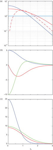
Also shown in Fig. 2a is the sum of the first three terms in eq. (33). The prediction of the SLM by eq. (33) is qualitative in nature because of the truncation of the expansion. Nevertheless, one can see that this equation predicts the correct behaviour in so far as it explains that the SLM should have less growth than the TLM for states less than 1 and more growth for states greater than 1. Note that for our example problem T ₀₀=0 and therefore the structure in eq. (33) is determined entirely from the third term on the right-hand side. In figure 2b we plot the associated structure of the TLM and its first and second derivatives as required by eq. (33). Here we can see that the change in sign of explains the change in behaviour of the SLM from predicting less growth as compared to the TLM for states less than 1 and more growth for states greater than 1.

Lastly, we compare the estimates of the variance by the TLM and the SLM. In Fig. 2c, we show the t=1 variance obtained by centring a very large ensemble (10⁷ members) at different values of the state, integrating this forward to t=1, and subsequently calculating the sample variance. We take this as the true variance at t=1. In Fig. 2c, we evaluate the t=1 estimate of the variance by the TLM by evaluating the quantity M ₁₀ P ₀₀ M ₁₀ for different values of . We also plot in Fig. 2c the estimate of the variance by the SLM, i.e. . The point of this figure is that the SLM produces a better estimate of the true final time variance than the explicit TLM. Nevertheless, this does not change the fact that the quantity obtained from the TLM is the exact quantity required by an incremental/Gauss–Newton method to find the mode. Further evidence that this is so is found in Fig. 3. In Fig. 3, we show where the incremental/Gauss–Newton method converges if the TLM is replaced by the SLM and iterated to convergence.

Fig. 3 Convergence curves. The result of outer loop iterations in the incremental method using a TLM (blue), SLM derived using the true prior (red), and SLM derived using a reduced prior variance (red dashed). The horizontal black line is the posterior mode; horizontal cyan line is posterior mean; and horizontal green line is the state estimate obtained from the BLUE of Section 3.

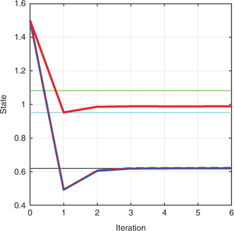
The SLM leads to convergence, but to neither the posterior mode nor mean. In addition, we also show in Fig. 3 where the first step of the incremental method lands using the TLM or SLM. Note that the first step for the SLM happens to land nearer to the true posterior mean than the BLUE. Other choices for the value of the observation find that the first iteration does not always land near to the true posterior mean (not shown).

Therefore, the SLM generally delivers a state estimate from the incremental method nearer to the BLUE than the TLM. By contrast, however the first step of the incremental method using the TLM does not find a reasonable approximation to the BLUE, because the estimate of the final time variance by the TLM is not accurate (recall Fig. 2c). Lastly, we replace the SLM derived using the true prior with an SLM that is derived using a prior whose variance is reduced by a factor, ɛ=0.1, in the incremental method of Section 4.A to find the mode. Figure 3 shows that this method does in fact converge to the mode given that the factor, ɛ, is small enough. Larger values of ɛ were found to provide a poor convergence to the mode (not shown). Deriving an SLM using a prior with a reduced variance can be considered an example of the method in Sakov et al. (2012) and Bocquet and Sakov (2014).

6. On the ‘Strong-Constraint’ TLM test

Our goal in this section is to compare the strong-constraint TLM test for TLMs and SLMs as applied to prior perturbations and to analysis corrections. We wish to show that standard tests for the TLM and SLM are well-defined for prior perturbations, but it is less clear what they mean for analysis perturbations. This is important because it is not uncommon for articles on strong-constraint 4D-Var and ensemble Kalman smoother data assimilation to attempt to test the analyses output across a data assimilation window. Often the test is made to pertain to a single observation correction or analysis increments (e.g. Tremolet, 2004; Lorenc et al., 2015). Our goal here is to show that the analysis states that are output at different times across an assimilation window, whether the method is strong-constraint 4D-Var or a method attempting to calculate the BLUE, do not follow a trajectory of the non-linear model, even though they are referred to as ‘strong-constraint’. We will begin with the mode-finding discussion followed by the BLUE-finding discussion.

6.1. TLM tests using the prior

A standard measure of the linearity of a particular physical system is to determine the relative error (e.g. Tremolet, 2004):39

where, because the quantities here are scalars, we take the norm in eq. (39) represented by the vertical bars to simply be the absolute value. Using eq. (24), we immediately find that eq. (39) can be approximated by40

which is a recapitulation of the conditions [eqs. (14)–(16)]. Therefore, if the TLM, M ₁₀, used in eq. (39) is the true TLM then the test in eqs. (39 and 40) is a measure of the linearity of the model dynamics [eq. (2)] and therefore the smallness of r is determined by the conditions [eqs. (15) and (16)].

The test [eq. (39)] is typically used in two different ways to measure the quality of the TLM and SLM. In the first way, one might use a flawed TLM, , in eq. (39). This would result in an additional term in eq. (40) such that41

Therefore, the magnitude of r is now determined by both the linearity of the physical system as well as the quality of the flawed TLM. Tuning the TLM to minimise eq. (41) should result in a better TLM.

The second way relative error measures like eq. (40) are used is to assess the quality of SLMs. To assess the quality of the SLM, we must translate eq. (28) into a relative error measure by redefining the vertical bars in eq. (39) as meaning the square of the quantity (and of course integrate with respect to the joint prior) such that

where

Note that in the derivation of eq. (42) from eq. (43) we have made the strong-constraint assumption in the transition density in order to arrive at relative error measures consistent with those presented in Lorenc and Payne (2007) and Payne (2013). If the SLM [eq. (29)] is used in the relative error norm [eq. (42)], then

which should be compared to eq. (9) with R=0. If the SLM's prediction, , of the t=1 prior variance, P ₁₁, is accurate, the relative error norm is small. In Section 5, we showed that the SLM generally does a good job of predicting the final time variance and therefore a reasonable method to tune a SLM is on the smallness of eq. (42) with respect to prior perturbations.

6.2. TLM tests using the analysis

6.2.1. Mode-finding methods.

A typical ratio test requires that we output analysis states for at least two different times, which we will refer to as and , and use in an equation of the form:

where and is typically taken to be the prior mean or background forecast. The issue we wish to discuss here for mode-finding methods is how to write out the state and what does it mean when we do.

We begin by noting that the 4D forecast error covariance matrix implied by the gain matrix for the mode in eq. (19) is the prior covariance matrix from the TLM [eq. (23)]. The prior covariance matrix from the TLM [eq. (23)] also gives the 4D covariance matrix that would be used by an EKS. Again, this is different from that in eq. (4). Clearly, in the prior covariance matrix from the TLM [eq. (23)] the second element in each column is the first element in that same column propagated forward using the TLM. This implies that a single observation increment from a 4DVar scheme can be thought of as being propagated from time 0 to time 1 using the TLM. Moreover, the increment from many observations can be thought of as a weighted, linear combination of the columns of eq. (23) each of which can be thought of as connected through time by the TLM.

Equation (19) only produces a state estimate at t=0. How then can one apply the relative error norm [eq. (19)], which requires the state at time t=1? This analysis correction through time is apparently produced by analogy with the Kalman smoother formula:

A single observation increment of eq. (46), which simply makes use of one column of eq. (19), is not connected through time by the non-linear model. It is connected through time by the linearised model. This begs the question: if the mode is a trajectory from t=0 to t=1 of the non-linear model and the result of eq. (46) is not, then is eq. (46) delivering anything of significance at t=1? If not, then what is being measured by comparing non-linear model simulations with analysis corrections from eq. (46) in the relative error measure [eq. (45)]?

To answer these questions, we must return to the fundamental Bayesian framework that we operate from. We begin by writing Bayes’ rule for the joint posterior

where we recall that p(x ₀) is N(1.5,1), p(y ₁∣x ₁) is N(x ₁,R), and p(x ₁∣x ₀) is the transition density for the model [eq. (3)]. Note that the transition density for the model in eq. (3) is a Dirac delta function because we have assumed that the model is deterministic. When the transition density is a Dirac delta it becomes unclear how to extract a cost function from eq. (47). Therefore the standard procedure of minimising the negative logarithm to find the mode of the joint posterior will not work.

How then does the standard cost function [eq. (4)] relate to eq. (47)? The answer is through the marginalisation process. To marginalise the joint density for t=0, one would integrate with respect to x ₁ to find the marginal density

where we note that

The object p(y ₁∣x ₀) is Gaussian with mean x ₁(x ₀) and variance equal to R. Using this fact and taking the negative logarithm of eq. (49) obtains eq. (10). Hence, the minimum we obtained in Section 3 was the mode of eq. (48), and therefore the solution to eq. (10) obtains the mode of the marginal posterior at t=0.

By contrast, the PDF of the marginal posterior at time 1 is

where we note that

Even though p(x ₀) is Gaussian, p(x ₁) is not when the model is non-linear. Therefore, because p(x ₁) is in general non-Gaussian the quantity referred to in eq. (46) and denoted by is an incorrect formula for the mode of the joint or the marginal posteriors at time 1; in fact it is only equal to the mode at time 1 when the model dynamics are linear. This implies that there can be no expectation that the non-linear model will propagate to the quantity defined in eq. (46); whether this is true or not depends only on whether or not the model [eq. (2)] is linear and not necessarily on the quality of our data assimilation system or even on the quality of the TLM.

Let's make these ideas more concrete by comparing the marginal to the joint posterior for our simple example problem. In Fig. 4a, we plot the prior joint density which is equal to

Fig. 4 The joint prior and posterior are shown in (a) and (b), respectively. The black line shows how the model links x₀ with x₁. The colours represent the density. The horizontal and vertical lines denote the location of the mode of the joint posterior. The marginal prior and posterior are shown in (c) and (d), respectively. Blue (red) is t=0 (t=1). In (d), the vertical black (dashed) line is the mode at t=0 (t=1). The vertical green line is the estimate of the mode at t=1 using eq. (11). In (e) is plotted the TLM as a function of different reference states in blue and its inverse in red.

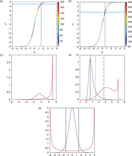
Because the transition density is the Dirac delta we find that the joint density is non-zero only precisely along the line defined by the model [eq. (2)]. Technically, eq. (52) has an infinite value along this line because the Dirac delta is infinite along this line. The value of the PDF denoted in Fig. 4a can be thought of as a kind of coefficient that we attach to a Dirac delta in this plane and is determined by the structure of p(x ₀) and the structure of our non-linear model. The mode of this joint density, identified in this way, is a trajectory of the model and denoted in this figure. Given eq. (52), we may evaluate eq. (47) for the joint posterior and this is evaluated in Fig. 4b for our example observation of y₁=2.5. Here we see that the mode has moved towards the observation and the spread of colours along the line denoting the model has contracted indicating that the variance has decreased because we assimilated an observation.

We may also calculate the marginal prior and posterior and compare these to the joint densities. The marginal densities are plotted in Fig. 4c and d. Note that the mode of the marginal density at t=0 is identical to the mode of the joint density at t=0. However, the mode at t=1 of the marginal density is not equal to the mode of the joint at t=1. By contrast, note that the mode of the joint at t=1 is connected to the mode of the joint at t=0 by the non-linear model. The mode of the marginal is not connected by the non-linear model because of the integration we performed to derive the marginal. One way to understand the impact of this integration on the structure of the marginal is to write the marginal at t=1 using a variable transformation, viz.

where we have used the fact that the model [eq. (3)] has a known inverse in order to calculate x ₀(x ₁). The quantity ∣dx ₀/dx ₁∣ is the determinant of the Jacobian (inverse of the TLM) and is plotted in Fig. 4e. Equation (53) shows that the mode of p(x ₁) is not simply the mode of p(x ₀) mapped forward in time, because of the multiplication by the determinant of the Jacobian whose structure modifies the location of the mode. This multiplication by the determinant of the Jacobian accounts for the convergence/divergence of the models trajectories through state space in the marginalisation process.

We have therefore shown that the only object in this framework that is connected through time by the non-linear model is the modes of the prior and posterior joint densities. However, eq. (46) is not the formula for either of these objects.

6.2.2. BLUE-finding methods.

All of these same notions seen in the previous section also apply to the BLUE of Section 3. One cannot create the BLUE at two different times and expect that they are connected precisely by the non-linear model, even in the strong-constraint case. Note that the analysis for the BLUE at both t=0 and t=1 for our example problem is from eq. (6):

If we use these analyses in eq. (45), we would be assuming that BLUE analyses are connected through time by the non-linear model. In this section, we will be testing whether or not this assumption is valid.

In eqs. (54) and (55), we see that the observation increments at the two times are simply a number times the elements of the second column of eq. (4). Therefore, if one expects that the BLUE is connected through time by the non-linear model this implies that one also expects that the second column of eq. (4) could be created using the non-linear model. This is proportional to a single observation increment for an observation at time 1 and a state update at time 0, and we would be expecting that this single observation increment would be linked through time by the non-linear model.

The way we will test this is to use the covariance through time, P ₀₁, as a perturbation at the initial time of the prior mean. We then integrate this new state under the dynamics of the non-linear model [eq. (3)] and subtract this state at t=1 from the unperturbed state also integrated forward to t=1. The resulting quantity is supposed to be the correct final time variance, P ₁₁, or equivalently proportional to the single observation correction at time 1. If this were true, then the ratio test in eq. (45) would vanish, implying that BLUE state estimates are trajectories of the non-linear model in the strong-constraint problem.

We can test if this is so in our simple example model problem. The perturbed state consists of , where we have added the covariance through time to the prior mean at t=0 [as in eq. (54)] and have set the constant α=1. Setting α=1 results in a state that is identical to that which would be obtained from a single observation BLUE correction in the case that the innovation divided by the innovation variance was equal to unity.

Next, we propagate this state forward in time using the non-linear model [eq. (3)]. This obtains . The unperturbed state is and when propagated with the non-linear model yields . Therefore, this test of the covariance matrix results in the value 0.48 for the final time state estimate, even though the correct value is 3.49 as revealed by eq. (4). Additionally, one may use these values in eq. (45) to evaluate the ratio test, which obtains r=6.3, which is a very poor result for a ratio test. Note however that the analysis determined from eq. (54) and (55) is the exact BLUE with no approximations. Therefore, one cannot test BLUE-finding methodologies using the ratio test in eq. (45).

This analysis shows that this technique to test the quality of one's 4D covariance matrix, or equivalently the quality of the corrections to the prior forecast by a data assimilation algorithm that is constructed to approximate the BLUE, is a test of the linearity of one's physical system but has nothing to do with revealing whether one has the correct covariance matrix to obtain the BLUE. The reason is that a non-linear model implies that (1) computing a covariance and applying the model/observation operator do not commute; and (2) that superposition does not hold. In other words, one must propagate forward an ensemble (i.e. the distribution under consideration) from the initial time to the final time to calculate the final time variance. One cannot calculate the covariance between time levels, P ₀₁, and then, after the covariance calculation, apply the non-linear model. This is essentially a reversal of the order of the steps of the calculation of the final time variance and this kind of reversal can only work when the physical system under consideration is linear and therefore the model operator commutes.

7. Summary and conclusions

The 4D forecast covariance matrix used to find the BLUE is not the same covariance matrix required to find the mode using an incremental/Gauss–Newton method. We showed that, while the algorithm (either Gauss–Newton or incremental) appears similar in form to an ensemble Kalman smoother, in the presence of non-linear error dynamics, the forecast covariance matrix within it is an entirely different object from the one within an ensemble Kalman smoother. This has important ramifications to not only the design of the data assimilation algorithm but also to its tuning and validation.

We showed that standard methods find different state estimates and the algorithm designer must be cognizant of this fact:

1. To find the mode, one needs the 4D forecast error covariance matrix obtained by propagating the prior distribution using purely linear dynamics and then taking the covariance of the resulting 4D perturbations. A 4DVar outer loop is required to obtain the mode of the posterior distribution; this also means one must use a modified innovation as in eq. (19).

2. To find the BLUE, one needs to propagate the prior distribution using the full non-linear model and then take the covariance. Given this covariance matrix for the true prior one evaluates eq. (6) and does not use an outer loop. 4DEnVar with no outer loop and the ensemble Kalman smoother find an approximation to the BLUE.

3. Regardless of whether a 4DVar scheme employs a hybrid static/ensemble covariance matrix or not, 4DVar algorithms do not find the BLUE if those schemes make use of the TLM for the 4D covariance structure. They can, however, be used to find the mode of the posterior at the beginning of the window for strong constraint if they employ an outer loop.

4. The use of an SLM can be used to find a better estimate of the BLUE than the use of the TLM, but the SLM cannot be used to determine the mode of the posterior unless it is re-derived using a ‘prior’ distribution with infinitesimal error variance (as in Sakov et al., 2012). We see no obvious reason for performing outer loops with a non-infinitesimal SLM because the iteration would lead to a state that was neither the BLUE nor the mode. Further research is required to understand what it means to perform an outer loop in this case.

5. Lastly, we showed that for mode-finding methods one cannot, in general, expect the linear trajectory of states obtained by propagating the most likely analysis state through time using the linear model to be the same as the corresponding sequence obtained from the non-linear model. Similarly, one should not expect a sequence of states obtained from BLUE-finding methods to correspond to a non-linear model trajectory either. This calls into question the practice of testing data assimilation algorithms using ratio tests on single observation corrections and analysis increments.

Some numerical weather prediction centres do not perform an outer loop in their variational data assimilation schemes. Without an outer loop, the 4DVar apparatus employed at these centres will better approximate an EKS analysis than a mode when non-linearity is present. A primary reason that an outer loop is not performed at these centres is that the computational cost of the outer loop has been found to outweigh its benefits. For the reasons discussed above, the analysis given by 4DVar without an outer loop would be more similar to the BLUE estimate if the TLM was replaced by an SLM. This suggests that if ensemble-based SLMs could be derived that provided good approximations to the true SLM at an affordable computational cost, then centres that perform 4DVar without an outer loop might actually realise accuracy gains by replacing their TLMs with SLMs and re-focusing their efforts towards finding the BLUE.

Another approach to getting 4D variational data assimilation schemes that were originally designed to find modes to find the BLUE is to simply incorporate within them 4D ensemble covariance matrices. Unlike the SLM approach, this approach enables the prior ensemble covariances to define the forecast error covariance through time. This feature makes this approach more like the BLUE than that which would be obtained by using a SLM because it is directly based on the 4D covariances of an ensemble of non-linear forecasts. The key practical challenges of this approach include how the covariances should be localised through time (Bishop and Hodyss, 2011) and how to accommodate a hybrid covariance matrix that blends climatological error covariance information with error covariance information from the ensemble. Future research will be needed to tell whether SLMs or those based on localised 4D ensemble covariance matrices would best enable a 4DVar type scheme to find the BLUE, and whether finding the mode or the BLUE of the posterior is best for geophysical applications.

8. Appendix A

A.1. The Gauss–Newton algorithm

One way to solve eq. (10) for its minimum is the Gauss–Newton algorithm. This requires access to the Jacobian matrix of the cost function [eq. (10)], which for our problem is simply a scalar,

as well as the Hessian matrix, which is again here a scalar,

The basic assumption of the Gauss–Newton algorithm is that the last term on the right-hand side of (A2) can be neglected. This assumption is valid when the model dynamics is only weakly non-linear and/or the state x₁ is close to the observation y₁ at the minimum. Note that both these assumptions are equivalent to the assumptions in eqs. (15) and (16), respectively. The result of this assumption is that convergence is not guaranteed.

In any event, the minimum of eq. (10), which we denote as , is found iteratively through the following formula:

where the superscripts in (A3) denote the ith iteration, and we remind the reader that we use the approximate Hessian neglecting the last term in (A2). Equation (A3) is simply obtained by writing a Taylor-expansion around for dJ/dx ₀ at and then finding the value of that makes dJ/dx ₀=0. Inserting (A1) and (A2) into (A3) obtains eq. (19).

9. Appendix B

B.1.The posterior variance about the mode

In this appendix, we briefly discuss how the posterior variance about the mode relates to the structure of the cost function. The posterior variance calculated about the mode is

where we note for completeness that

and is the true posterior mean at t=0. Note that given eq. (10) that we may represent the posterior density in (B1) asB4

where N is simply a normalisation constant. We may make use of the representation in (B4) to understand (B1) by writing the cost function as a Taylor-series about the mode, viz.B5

where it is understood that the derivatives in (B5) are evaluated at the mode. Note that the term proportional to the first derivative is absent as it vanishes when evaluated at the mode. Furthermore, because the cost function is a minimum at the mode we know that . Lastly, the presence of the cubic term in (B5) implies an asymmetry in the cost function such that the posterior (B4) will be left (right) skewed when (). This skewness of the posterior as well as any other non-Gaussian structure is always a result of non-linearity in the model or the observation operators.

As an example, when the cost function in eq. (4) is quadratic, which implies a linear model or observation operator, all derivatives higher than the second vanish in (B5). Hence, eq. (B1) becomesB6

where the term has been absorbed into the normalisation constant, N. In this case, we know that the result of (B6) is that the variance is equal to the inverse of the Hessian. By contrast, whenever the cost function differs from quadratic (i.e. a non-linear model or observation operator) the derivatives higher than the second no longer vanish in (B5) and therefore the inverse Hessian is no longer equal to the posterior variance. As we have shown in Section 3, this effect is not small as the estimate of the posterior variance about the mode (B1) by the inverse Hessian is in error by an order of magnitude.

References

- Bennett A. F . Inverse modeling of the ocean and atmosphere. 2002; Cambridge University Press, Cambridge, United Kingdom. 256.
- Bishop C. H. , Hodyss D . Adaptive ensemble covariance localization in ensemble 4D-Var state estimation. Mon. Weather Rev. 2011; 139: 1241–1255.
- Bocquet M. , Sakov P . An iterative ensemble Kalman smoother. Q. J. Roy. Meteorol. Soc. 2014; 140: 1521–1535.
- Buehner M. , Houtekamer P. L. , Charette C. , Mitchell H. L. , He B . Intercomparison of variational data assimilation and the ensemble Kalman filter for global deterministic NWP. Part I: description and single-observation experiments. Mon. Weather Rev. 2009; 138: 1550–1566.
- Buehner M. , Morneau J. , Charette C . Four-dimensional ensemble-variational data assimilation for global deterministic weather prediction. Nonlin. Processes Geophys. 2013; 20: 669–682.
- Clayton A. M. , Lorenc A. C. , Barker D. M . Operational implementation of a hybrid ensemble/4D-Var global data assimilation system at the Met Office. Q. J. Roy. Meteorol. Soc. 2013; 139: 1445–1461.
- Courtier P . Dual formulation of four-dimensional variational assimilation. Q. J. Roy. Meteorol. Soc. 1997; 123: 2449–2461.
- Courtier P. , Thépaut J.-N. , Hollingsworth A . A strategy for operational implementation of 4D-Var, using an incremental approach. Q. J. Roy. Meteorol. Soc. 1994; 120: 1367–1387.
- El Akkraoui A. , Gauthier P. , Pellerin S. , Buis S . Intercomparison of the primal and dual formulations of variational data assimilation. Q. J. Roy. Meteorol. Soc. 2008; 134: 1015–1025.
- Errico R. M. , Raeder K . An examination of the accuracy of the linearization of a mesoscale model with moist physics. Q. J. Roy. Meteorol. Soc. 1999; 125: 169–195.
- Errico R. M. , Vukicevic T. , Reader K . Examination of the accuracy of a tangent linear model. Tellus A. 1993; 45: 462–477.
- Fairbairn D. , Pring S. R. , Lorenc A. C. , Roulstone I . A comparison of 4DVar with ensemble data assimilation methods. Q. J. Roy. Meteorol. Soc. 2014; 140: 281–294.
- Gauthier P . Chaos and quadri-dimensional data assimilation: a study based on the Lorenz model. Tellus. 1992; 44A: 2–17.
- Jazwinski A. H . Stochastic Processes and Filtering Theory. 1970; Inc., Mineola, New York: Dover Publications. 376.
- Kleist D. T. , Ide K . An OSSE-based evaluation of hybrid variational–ensemble data assimilation for the NCEP GFS. Part II: 4DEnVar and hybrid variants. Mon. Weather Rev. 2015; 143: 452–470.
- Klinker E. , Rabier F. , Kelly G. , Mahfouf J.-F . The ECMWF operational implementation of four dimensional variational data assimilation. Experimental results and diagnostics with operational configuration. Q. J. Roy. Meteorol. Soc. 2000; 126: 1191–1215.
- Kuhl D. D. , Rosmond T. E. , Bishop C. H. , McLay J. , Baker N. L . Comparison of hybrid ensemble/4DVar and 4DVar within the NAVDAS-AR data assimilation framework. Mon. Weather Rev. 2013; 141: 2740–2758.
- Le Dimet F.-X. , Talagrand O . Variational algorithms for analysis and assimilation of meteorological observations. Tellus A. 1986; 38: 97–110.
- Lewis J. M. , Lakshmivarahan S. , Dhall S. K . Dynamic data assimilation: a least squares approach. 2006; , Cambridge: Cambridge University Press. 654.
- Li Z. , Navon I. M . Optimality of variational data assimilation and its relationship with the Kalman filter and smoother. Q. J. Roy. Meteorol. Soc. 2001; 127: 661–683.
- Lorenc A. C . Analysis methods for numerical weather prediction. Q. J. Roy. Meteorol. Soc. 1986; 112: 1177–1194.
- Lorenc A. C . Development of an operational variational assimilation scheme. J. Meteorol. Soc. Jpn. 1997; 75: 339–346.
- Lorenc A. C . Modelling of error covariances by 4D-Var data assimilation, Q. J. Roy. Meteorol. Soc. 2003a; 129: 3167–3182.
- Lorenc A. C . The potential of the ensemble Kalman filter for NWP – a comparison with 4D-Var. Q. J. Roy. Meteorol. Soc. 2003b; 129: 3183–3203.
- Lorenc A. C. , Payne T . 4D-Var and the butterfly effect: statistical four-dimensional data assimilation for a wide range of scales. Q. J. Roy. Meteorol. Soc. 2007; 133: 607–614.
- Lorenc A. C. , Bowler N. E. , Clayton A. M. , Pring S. R. , Fairbairn D . Comparison of hybrid-4DEnVar and Hybrid-4DVar data assimilation methods for global NWP. Mon. Weather Rev. 2015; 143: 212–229.
- Mahfouf J.-F. , Rabier F . The ECMWF operational implementation of four dimensional variational data assimilation. Experimental results with improved physics. Q. J. Roy. Meteorol. Soc. 2000; 126: 1171–1190.
- Navon I. M. , Zou X. , Derber J. , Sela J . Variational data assimilation with an adiabatic version of the NMC spectral model. Mon. Weather Rev. 1992; 120: 1433–1446.
- Payne T. J . The linearization of maps in data assimilation. Tellus A. 2013; 65: 18840.
- Pedlosky J . Geophysical Fluid Dynamics. 1987; Springer, New York. 710.
- Rabier F. , Järvinen H. , Klinker E. , Mahfouf J.-F. , Simmons A . The ECMWF operational implementation of four-dimensional variational assimilation. I: experimental results with simplified physics. Q. J. Roy. Meteorol. Soc. 2000; 126: 1143–1170.
- Rabier F . Overview of global data assimilation developments in numerical weather-prediction centres. Q. J. Roy. Meteorol. Soc. 2005; 131: 3215–3233.
- Rawlins F. , Ballard S. P. , Bovis K. J. , Clayton A. M. , Li D. , co-authors . The Met Office global four-dimensional variational data assimilation scheme. Q. J. Roy. Meteorol. Soc. 2007; 133: 347–362.
- Rosmond T. , Xu L . Development of NAVDAS-AR: non-linear formulation and outer loop tests. Tellus A. 2006; 58: 45–58.
- Sakov P. , Oliver D. S. , Bertino L . An iterative EnKF for strongly nonlinear systems. Mon. Weather Rev. 2012; 140: 1988–2004.
- Talagrand O. , Courtier P . Variational assimilation of meteorological observations with the adjoint vorticity equation. I: theory. Q. J. Roy. Meteorol. Soc. 1987; 113: 1311–1328.
- Tarantola A . Inverse problem theory and methods for model parameter estimation. 2005; , Philadelphia: Society for Industrial and Applied Mathematics. 342.
- Tremolet Y . Diagnostics of linear and incremental approximations in 4D-Var, Q. J. Roy. Meteorol. Soc. 2004; 130: 2233–2251.
- Wang X. , Lei T . GSI-based four-dimensional ensemble-variational (4DEnsVar) data assimilation: Formulation and single-resolution experiments with real data for NCEP global forecast system. Mon. Wea. Rev. 2014; 142: 3303–3325.
- Zhang X. , Huang X.-Y. , Liu J. , Poterjoy J. , Weng Y. , co-authors . Development of an efficient regional four-dimensional variational data assimilation system for WRF. J. Atmos. Oceanic Technol. 2014; 31: 2777–2794.