Air–lake boundary layer and performance of a simple lake parameterization scheme over the Tibetan highlands

Abstract

The Tibetan Plateau (TP) is covered by thousands of lakes which affect the regional and global heat and mass budget with important implications for the current and future climate change. However, the heat and mass budget of TP lakes and the performance of contemporary lake models over TP have not been quantified to date. We utilise 3-yr observations from Ngoring Lake, the largest lake in the Yellow River source region of TP, to investigate the typical properties of the lake–air boundary layer and to evaluate the performance of a simplified lake scheme from the Community Land Model version 4.5 (SLCLM) as one of the most popular lake parameterization schemes in atmospheric models. The strong boundary layer instability during the entire open-water period is a distinguishing feature of the air–lake exchange, similar to the situation over tropical and subtropical lakes, while contrasting to the generally stable atmospheric conditions commonly observed over ice-free temperate and boreal lakes from spring to summer. The rather simple algorithm of SLCLM demonstrated good performance in these conditions. A series of sensitivity simulations with SLCLM revealed strong shortwave solar radiation and cold air temperatures because of high altitude as the primary factors causing the boundary layer instability. The outcomes of the study (1) demonstrate the role of TP lakes as accumulators of shortwave solar radiation releasing the heat into the atmosphere during the entire open-water period; (2) justify the use of simple lake models for the Tibetan highlands, while revealing remarkable uncertainties in the estimations of the latent heat flux; (3) qualify the strong cool-skin effect on the lake surface which results from permanent negative air–lake temperature difference, and should be taken into account when interpreting remote sensing data from highland areas.

• unstable boundary layer
• air–lake interaction
• Ngoring Lake
• CLM
• lake modelling
• Tibetan Plateau

1. Introduction

The Tibetan Plateau (TP), with a mean height of 4000m above sea level (asl), is the highest plateau on earth and harbours the largest number of high-altitude lakes worldwide. The lake network covers nearly 50 000km², including more than 1091 lakes with individual areas more than 1km², and amounts to ~49.4 % of the total lake area of China (Jiang and Huang, 2004). Evidence has recently been reported with respect to an increase in the number of lakes on the TP (total of approximately 32843 lakes and 1204 lakes with an area over 1km²) related to global warming effects and local anthropogenic activity (Zhang et al., 2014). Along with the increasing number of small permafrost lakes and ponds, the large lakes are expanding because of the regional effects of the warming climate such as precipitation increase and accelerated glacier melt. Lakes have a significant feedback effect on local and regional climate (Stepanenko et al., 2010; Subin et al., 2012), and their climatic role increases with increased amount and areas. Compared to other regions with high numbers of lakes, such as Fennoscandia, Siberian Tundra, Northern Canada and south China (Xiao et al., 2013), the lakes of the TP are less investigated but apparently have an extraordinary thermal regime because of strong seasonal and synoptic variations.

The particular climatic environment of the TP creates a unique land–atmosphere interaction, including a lake–atmosphere interaction. Therefore, the lakes of the region have recently received increased attention. The availability of remote sensing data allows bulk estimation of changes in water level, area and the lake surface skin temperature (T _s). Studies on the lake effect on the regional water budget suggest that evaporation from one of the largest Tibetan lakes, Nam Co, provides up to 28.4–31.1 % of the local atmospheric water vapour content during the summer monsoon season (Xu et al., 2011), whereas the annual evaporation from Nam Co Lake exceeds annual precipitation and evaporation from the surrounding land (Haginoya et al., 2009). Simulations suggest that the different surface heat and mass budget over lakes could increase the regional precipitation over TP, including snow and rain (Li et al., 2009; Wen et al., 2015).

Direct field observations of the surface heat and mass budgets of lakes on the TP are extremely rare because of the harsh environmental conditions. Biermann et al. (2014) conducted a short-term field experiment on turbulent fluxes over a shallow lake within the basin of Nam Co Lake and demonstrated pronounced differences in eddy covariance (EC) fluxes over the lake and nearby grassland. The characteristics of energy flux and radiation balance over Ngoring Lake were investigated using a similar approach by Li et al. (2015) during two field campaigns covering several summer months of 2011 and 2012. The most remarkable feature of the lake–atmosphere heat exchange on the TP revealed by these recent studies is the persistent unstable air–lake boundary layer that appears throughout the open-water period. In lowlands, the long-lasting unstable boundary layer is more typical for tropical and subtropical lakes (Verburg and Antenucci, 2010) than for temperate and boreal lakes with strong seasonality (Long et al., 2007; Rouse et al., 2008), and implies strong effects on the energy transport from the lake surface. On the TP, a persistently unstable atmosphere has been observed over Ngoring Lake during the most part of the ice-free period (Li et al., 2015), as well as over a small lake nearby Nam Co Lake (Wang et al., 2015). Wang et al. (2015) analysed data from a single year, while Li's (2015) study combined observations from two subsequent summers that started in the middle of June, missed the early open-water period immediately after the ice-off and only show the daily mean characteristics. The study of Verburg and Antenucci (2010) on Lake Tanganyika demonstrated that an unstable atmosphere could increase the annual mean latent heat flux (LE) to 13 % and the sensible heat flux (H) loss to 18 % compared to the condition with the assumed neutral atmospheric boundary layer. In contrast, heat loss from the North American Great Lakes has been effectively suppressed by stable atmospheric conditions until late autumn (Long et al., 2007; Rouse et al., 2008). Hence, boundary layer stability is highly important for energy partitioning and affects different characteristics of the energy and mass budget over a lake surface, which should be quantified when upscaling the lake effects on the regional climate and water balance.

Stability of the atmospheric boundary layer is directly related to the temperature difference between the lake surface and air ΔT _sa=T _s–T _a (where T _a is the air temperature above the lake surface). ΔT _sa varies over the TP in a wide range on diurnal to seasonal scales. Up to now, variations in ΔT _sa over short time intervals and seasonal variations, especially the conditions in spring after the ice-off, remain unknown. The latter period is of special interest for understanding the lake effects on regional atmospheric conditions, as it is typically characterised by very stable atmospheric conditions because of faster warming of the surrounding land than the lake surface.

In addition, of special interest is the ability of conventional lake models to adequately simulate air–lake heat exchange and the internal lake thermal structure in the extreme conditions of the TP. A set of lake models has previously been validated over lowland lakes within the Lake Model Intercomparison Project (Stepanenko et al., 2010, 2014; Thiery et al., 2014b), demonstrating good ability of the models to simulate mixing processes and temperature distribution. Only a few lake models (Li et al., 2015; Wang et al., 2015) have been applied into high-altitude areas, but these models did not dynamically forecast the lake temperature, and the observed lake temperature was input and employed in the simulation (Li et al., 2015).

The present study investigates ΔT _sa over a typical Tibetan lake based on field experiments performed during several years over Ngoring Lake. The study has two major objectives:

• To quantify the characteristic of ΔT _sa (as a bulk stability characteristic to some extent) with different timescale, especially in late spring and early summer, over a typical TP lake and to investigate the mechanisms of its formation based on 3-yr observations.

• To evaluate the applicability of the bulk lake parameterization scheme in atmospheric models for modelling the thermal state of the TP lake and heat exchange between lake and air. The simplified lake scheme from the Community Land Model version 4.5 (SLCLM) was intentionally chosen for validation as a computationally cheap, yet robust and widely used lake model in atmospheric applications.

The study is based on data from a long-term field campaign covering the open-water season of 2013 starting from the early spring, and including EC measurements of turbulent heat fluxes complemented by the observations from 2011 to 2012, reported previously in part by Li et al. (2015). The observations are used to evaluate the performance of the SLCLM on the TP. Additional sensitivity experiments are performed to investigate the effect of different external parameters on the air–lake boundary layer characteristics.

2. Study area, observations and model

2.1. Study area

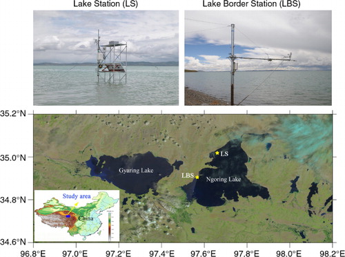
The Yellow River (also called Huang He) flows in and out of the Ngoring Lake, which is the largest lake (610km² surface area) in the Yellow River source region of the eastern TP. The mean (maximum) depth of the lake is 17 (32)m. With a lake surface altitude of 4274m asl and 0.05 % salinity, Ngoring Lake is a large freshwater lake at altitudes >4000m. The measured pH value is 8.49 and sampled lake water conductivity is 0.36–0.42mS cm⁻¹. Fish is rare in the lake, and aquatic plants grow only in the riparian area. Alpine meadows grow on the ground and low hills around the lake with a small seasonal variation in vegetation height (about 5cm).

The climate of the Ngoring Lake basin is cold semiarid continental. According to 1953–2014 data from the nearby Maduo weather station (34.9°N, 98.2°E) of the China Meteorological Administration, the mean annual temperature is −3.6 °C; the minimum, −16.2 °C, occurs in January and the maximum, 7.8 °C, in July; the average annual precipitation is 321.9mm with 85 % falling from May to September. Air temperatures remain relatively low in summer, with the daily maximum T _a over Ngoring Lake below 20 °C. Solar radiation in the Ngoring Lake basin is very strong owing to reduced optical thickness of the overlying atmosphere and even sometimes could exceed the solar constant. The longwave atmospheric radiation, Lwd, ranges between 200 and 400Wm⁻², which is only 50–70 % of that measured in the nearby low-altitude plain at ~1000 asl (Ji et al., 1995). The observed mean specific humidity (q) during the study period was about 0.004kg kg⁻¹, about 56 % of the saturated specific humidity. The surface pressure (ps) in the study area was as low as 600hPa. The observed wind speed (ws) over Ngoring Lake was relatively strong, ranging from 2 to 17m s⁻¹.

The lake is completely ice covered from late November or early December to April. In winter 2011–2012, winter precipitation (presumably snow because of the low air temperature) exceeded the long-term average. During the winter 2012–2013, the precipitation was in turn low, and snow barely covered the lake.

2.2. Observations

2.2.1. Lake station.

Lake station (LS) installed in Ngoring Lake in June 2011 at 35.03°N, 97.65°E (4274m asl) (Fig. 1) aimed at studying the mass and heat transfer over the lake. Logistical difficulties prevented installation of the observation platform in the deep centre of lake. Therefore, LS was situated in the north-western part of the lake standing up on a submerged rock about 200m away from the shore. The lake depth at the top of the rock exactly under the site was only 1m, increasing up to 3–5m within 200m distance of the site, and up to more than 15m at a distance of 1km from the site toward the lake centre. A small island was located 50m away to the southwest of the site. LS was damaged by ice in the winter 2011–2012. Afterward, LS was operated only during the open-water periods. The LS observations covered the periods from 29 June 2011 to 8 December 2011, from 7 June to 12 October 2012, and from 13 May to 10 September 2013, and included standard micrometeorological data (wind, T _a, q, ps), one-layer water temperature (T _w) about more than 0.1m below lake surface (the depth varied with the fluctuation of water level and could be deeper than 0.5m), four components of the radiation flux, H and LE. A Vaisala HMP45C temperature and humidity probe was used to measure T _a and specific humidity at a 3-m height over the lake surface. T _w was measured with a 109L probe (Campbell Scientific, Inc.). Downward shortwave radiation (Swd), Lwd, upward longwave radiation (Lwu) and upward shortwave radiation at a height of 1.5m over the lake surface were obtained with a net radiometer (CNR-1/CNR-4, Kipp and Zonen). An EC system, consisting of a three-dimensional sonic anemometer (CSAT3, Campbell Scientific, Inc.) and an open-path CO₂/H₂O infrared gas analyser (LI-7500/EC150, LI-COR/Campbell Scientific, Inc.), sampled fluctuations at 3m above the lake surface at 10Hz frequency. EC records were stored by the CR5000 data logger (Campbell Scientific, Inc.) and were processed to produce H and LE at 30-min intervals (see Li et al., 2015, for details). T _s was calculated from observed Lwd and Lwu as the following equation used in CLM4.5 model (Oleson et al., 2013) based on Stefan–Boltzmann Law:1 where σ=5.67×10⁻⁸Wm⁻² K⁻⁴ is the Stefan–Boltzmann constant, ɛ is the lake surface emissivity set to 0.97, the same as the community lake model (CLM) settings (Oleson et al., 2013).

Fig. 1 Study area map with locations of the observation stations (LB and LBS) and the photographs of the stations.

2.2.2. Lake border station.

In order to complement the LS observations and to ensure continuous records, especially during the wintertime, a long-term autonomous lake border station (LBS) was additionally installed in October 2012. LBS located on the southwestern lake shore (34.91°N, 97.55°E, 4282m asl), approximately 15km away from the LS, is currently in operation. The configuration and measured parameters at the LBS replicate those of the LS, except no T _w measurements. LBS represents well the water surface information during ice-free period and partly presents the lake surface during ice-covered period (Li et al., 2015).

2.2.3. Manual observations of lake ice thickness.

Lake ice thickness was manually measured at irregular intervals from December 2012 to March 2013 near the lakeshore, close to the LBS. The observed ice thickness remained above 0.6m from the middle of January to early March, with the maximum value (0.73m) measured in late February.

2.3. Lake model

We utilise the one-dimensional dynamic lake scheme of the CLM4.5 (Oleson et al., 2013), which is an improved version of the Hostetler et al. (1993) lake model. Originally, the lake scheme is coupled to the CLM4.5 model and has to be run under the Community Earth System Model (CESM) framework. To perform single-site simulations, the lake scheme was withdrawn from the CLM4.5 that caused decoupling from the surface albedo algorithm. In this form, the lake scheme has previously been applied to the Taihu Lake using net solar radiation input to avoid albedo calculations (Gu et al., 2013). In our study, the lake albedo was fixed as 0.06 for open-water conditions without considering the diurnal change as in CLM4.5, and calculated for an ice-covered lake with the following function (Mironov et al., 2010; Subin et al., 2012; Oleson et al., 2013):where T _f is the freezing temperature, and α _max and α _min are the maximum and minimum values of the lake ice albedo, respectively. In CLM4.5, there are different α _max (α _min) values for near infrared radiation and visible radiation. Without distinction between the two radiation types in the study, α _max and α _min were set to 0.6 and 0.1, respectively, as given by Mironov et al. (2010). For the sake of shortness, the modified model is called below SLCLM. Except for the abovementioned modifications, SLCLM was almost same as CLM4.5, including radiation transfer in the lake water. The β fraction of non-reflecting solar radiation into lake will be absorbed near the lake surface (about 0.6m). β is set to 0.4 without snow and calculated with snow optics submodel with resolved snow layers (Oleson et al., 2010; Gu et al., 2013). For ice-covered lake, the remaining solar radiation (1−α) Swd is absorbed in the top layer. For unfrozen lake, there is no radiation absorption in the top 0.6m except the surface, and the remaining solar radiation β(1−α) Swd is absorbed in the water according to the Beer–Lambert Law with a light extinction coefficient (Lec) η=η ₀ d ^−0.424, in which η ₀=1.1925, and d is the lake depth (Subin et al., 2012; Oleson et al., 2013). For the mean depth 17m of Ngoring Lake, η=0.35m⁻¹. Further details on the model configuration are given in Subin et al. (2012), Gu et al. (2013) and Oleson et al. (2013).

SLCLM dynamically calculates the lake–atmosphere heat balance and heat transport in the lake water body split in 10 water layers (Oleson et al., 2013). T _s is computed from the surface flux scheme. Using the surface net energy flux as the top boundary condition, vertical mixing of heat between the lake layers is parameterised as a function of wind-driven eddies, convection, molecular diffusion and enhanced diffusion intending to represent unresolved mixing processes (Fang and Stefan, 1996; Subin et al., 2012). Numerical solution of T _w is obtained with the help of the Crank–Nicolson thermal diffusion scheme. It should be noted that the thickness of the uppermost top lake layer is fixed to 0.1m in the lake scheme, regardless of changes in lake depth (>1m). The thicknesses of the remaining layers increase with a certain ratio from the surface to the lake bottom.

2.4. Methods of evaluating model performance

The performance of SLCLM over Ngoring Lake was quantified against observed temperatures and heat fluxes using three model efficiency scores, bias, root-mean-square error (RMSE) and the correlation coefficient (cc):3 4 5 where O _i represents the observations, n is the total number of observations and S _i represents the simulated results.

3. Observed characteristics of the air–lake boundary layer

The observations presented below cover the open-water periods of three consequent years; two of them, 2011 and 2012, have been analysed in detail by Li et al. (2015). The dataset of 2013 extends the previously available data by providing the boundary layer characteristics for the early stage of the open-water period, shortly after the ice melt, missing in previous years.

In the following brief overview of the measured boundary layer characteristics, we focus on the boundary layer stability, with particular attention to the seasonal and diurnal variations in the temperature difference between the lake surface and the lower atmosphere ΔT _sa and the temperature jump across the cool-skin layer at the lake surface T _s–T _w, as a bulk stability characteristic. For more detailed analysis, the reader is referred to Li et al. (2015).

Three-year observations at the LS show that air temperature T _a, water temperature T _w and skin temperature T _s had similar annual trends (Fig. 2), reaching a maximum in August followed by a gradual decline. T _a had the largest diurnal variation and the average of the variation exceeded 5 °C. The 3-yr observations consistently demonstrated that half-hourly T _s and T _w were predominately higher than T _a. Observations in 2013 further showed that the period of warmer T _s and T _w than T _a over ice-free Ngoring Lake could begin as early as the middle of May in spring, one month earlier than it was reported in the previous study (Li et al., 2015).

Fig. 2 Observed half-hourly T _a (grey line), T _w (red line) and T _s (green line, as calculated from the upward longwave radiation) at LS in (a) 2011, (b) 2012 and (c) 2013.

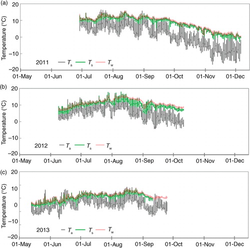
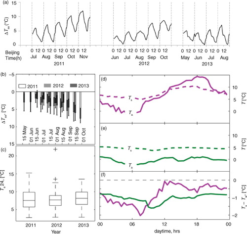
T _s and T _w in Ngoring Lake arrived at their maximum at around 15 °C in mid-August, decreasing afterward (Fig. 2). The air temperatures T _a followed the same seasonal trend with lower absolute values. The mean ΔT _sa was minimal in June, approximately 2–4 °C (Fig. 3ab). The differences in May were slightly higher than those in June, apparently because of the lower air temperatures. Later during the open-water season, ΔT _sa continued to increase, reaching the values of ~10 °C.

Fig. 3 (a) Observed monthly mean diurnal cycles of temperature differences between lake skin surface and air ΔT _sa; (b) 15-d mean temperature differences (bars) and standard deviations (lines) between the lake surface and air ΔT _sa in 2011–2013; (c) Box–Whiskers plot of diurnal Ta amplitudes T ₂₄ in the 3 years. The tops and bottoms of each ‘box’ are the 25th and 75th percentiles, respectively. The line in the middle of each box is the median. The whisker lengths correspond to±3 times standard deviation assuming normal distribution of the data with outliers marked as points; (d) diurnal course of air and lake surface temperatures on 12 June 2013 (the day with maximum diurnal T _a amplitude in 2013); (e) diurnal course of T _a and T _s on 16 May 2013 (the day with minimum diurnal T _a amplitude in 2013); (f) the cool-skin temperature drop for the day from (d) and (e).

Remarkably, the differences between the virtual air temperature and the virtual temperature of saturated air at the lake surface temperature ΔTv _sa were 1–2 °C higher than ΔT _sa because of the low air humidity and low air pressure (not shown). Hence, the humidity effect on stability of the air–lake boundary layer over Tibetan lakes appears even stronger than that reported previously by Verburg and Antenucci (2010) in the unstable boundary layer over tropical lakes.

Although lake temperatures were predominantly higher than air temperatures during all three observation periods of 2011–2013, short-term periods of stable boundary conditions appeared over the lake, especially at the beginning of the open-water period in May and June (Figs. 2bc and 3ab). For the entire observation period, stable conditions distinguished by ΔT _sa<0 were present in 10 % of observations and coincided roughly with periods with positive Monin–Obukhov stability parameter (not shown). The stable conditions usually appeared on the diurnal time scales following the diurnal oscillations of the air temperature: the mean daily amplitude of the T _a variations over Ngoring in May–September 2013 was 8.4 °C with a standard variation of 3.1 °C (Fig. 3b). The amplitude varied depending mostly on synoptic conditions without a distinct seasonal trend, except a slight tendency to decrease at the beginning of autumn cooling in August–September (Fig. 2). On 12 June 2013, the day with the strongest diurnal variations of air temperature, T _a varied from −2 °C in the late night to >14 °C during daytime (Fig. 3d). As a result, the difference (T _a−T _s) was positive for ~8 h, characteristic of stable boundary layer. An apparent reason for these stable events in early summer is the relatively rapid warming of the surrounding land by solar radiation with subsequent release of the heat to the atmosphere by infrared radiation. Later in summer, these events are rare, as the lake accumulates the heat from the solar radiation within its upper several meters because of high water transparency and remains warmer than the lower atmosphere even at sunny days. An intense heat release from the lake surface to the atmosphere is also able to produce a backward effect on the diurnal T _a variations by damping night-time air cooling, so that air temperatures remain nearly constant on daily time scales (Fig. 3e).

A distinguishing feature of the air–lake boundary layer over Ngoring is an appreciable cool-skin effect with typical differences between the bulk lake surface temperature and the radiative surface temperature of ~1 °C. In strongly unstable conditions, the difference between the bulk temperature and the skin temperature may reach 2 °C; during stable events at warm days, it reduces to zero (Fig. 3f). These values are essentially higher than typical cool-skin characteristics reported in the ocean (Fairall et al., 1996) and suggest strong effect of the viscous layer on the heat and mass exchange between the upper lake and the atmosphere.

Briefly summarised, the major challenges for parameterising of Tibetan lakes in atmospheric models are boundary layer instability, influence of low humidity and low atmospheric pressure on the latent heat exchange, and strong cool-skin effect.

4. Evaluation of the lake model performance for Ngoring Lake

Due to absence of observations in winter 2011–2012, only the period from 9 June 2012 to 23 August 2013 was studied with SLCLM. The model was forced with observations from the LS in June–October 2012 and May–September 2013, complemented with data from LBS from October 2012 to May 2013. In the following, the simulation is referred as control run (CTL), in which the lake depth set to 17m (the mean lake depth).

CTL captured well the observed time variations of T _s, T _w, ice thickness, H and LE (Fig. 4 and Table 1). The simulated daily mean values of T _s (Bias=1.4 °C, RMSE=1.6 °C, cc=0.95) and T _w (Bias=0.4 °C, RMSE=0.7 °C, cc=0.98) were close to but a little higher than observations. The simulated ΔT _sa was a little stronger than the observed one. The simulated maximum ice thickness was less than 0.1m thinner than in observations. The observed magnitudes and diurnal variations of H were fairly represented with a small overestimation (Bias=9.8Wm⁻², RMSE=14.7Wm⁻²), while overestimation of the latent heat flux, LE by the model was appreciably stronger (Bias=31.1Wm⁻², estimated for the period from June to October 2012 only, because of technical failure of water vapour measurements in 2013). The higher bias and RMSE in the simulated heat fluxes, especially LE, may be referred to two possible reasons: One is the currently used roughness length parameterization, which is based on ocean observations and could result in the simulated annual evaporation being 40 % higher than the observed values (Xiao et al., 2013). Another potential source of error stems from the observations: EC techniques have been shown to underestimate LE (Nordbo et al., 2011), which can reach up to 53 % (Elo, 2007). Generally, the SLCLM model simulated well the boundary layer characteristics over Ngoring Lake, except LE. The mostly positive ΔT _sa over the unfrozen lake could be represented and verified by the model. The SLCLM model performance for the generally persistent unstable atmosphere over the lake was further investigated by sensitivity runs with varying governing factors.

Fig. 4 (a) Observed (black solid line) and simulated (colour lines) T _s, (b) T _w, (c) ΔT _sa, (d) ice thickness, (e) H, and (f) LE in CTL (blue dash line) and sensitivity experiments Sd2 (red dotted line) and Sd32 (green line) with different lake depths.

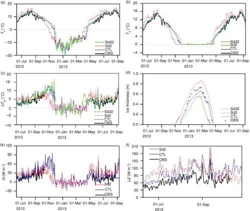
Table 1. Bias, RMSE and cc between simulation and observation

		T s	T w	H	LE	Ice thickness
Bias	Sd2	2.2 °C	1.2 °C	14.2Wm^−2	38.9Wm^−2	0.14m
	CTL	1.4 °C	0.4 °C	9.8Wm^−2	31.2Wm^−2	−0.05m
	Sd32	1.2 °C	0.2 °C	8.7Wm^−2	29.1Wm^−2	−0.21m
RMSE	Sd2	2.6 °C	1.9 °C	17.3Wm^−2	43.2Wm^−2	0.15m
	CTL	1.6 °C	0.7 °C	14.7Wm^−2	35.2Wm^−2	0.07m
	Sd32	1.5 °C	0.6 °C	14.1Wm^−2	33.9Wm^−2	0.21m
cc	Sd2	0.88	0.83	0.63	0.68	0.91
	CTL	0.95	0.98	0.70	0.86	0.97
	Sd32	0.94	0.98	0.70	0.85	0.91

cc, correlation coefficient; CTL, control run; H, sensible heat flux; LE, latent heat flux; RMSE, root-mean-square error; T _s, skin temperature; T _w, water temperature.

5. Model sensitivity to varying lake characteristics

5.1. Impact of variable lake depth

Sensitivity simulations with 2m (lake depth around LS) and 32m (maximum lake depth) lake depth, referred to as Sd2 and Sd32, respectively, were conducted to examine the effects of lake depth on the simulated results.

All simulations with different lake depths (Fig. 4) captured the observed seasonal pattern and sub-seasonal time variations of T _s, T _w, H and LE with the positive bias over ice-free period. The bias and RMSE of these variables reduced with increasing lake depth from Sd2, to CTL to Sd32, while simulated results in CTL had a higher cc with observations than those in Sd32. Also, the simulated daily variations of temperature, as well as the simulated ice thickness were closer to the observations in CTL than in Sd32. A general tendency in ice thickness simulations was ice thinning with increased lake depth from Sd2 to Sd32 because of the increase of the lake heat inertia with depth.

Values of all the analysed variables and the related model efficiency scores (bias, RMSE and cc) changed stronger between Sd2 and CTL than between CTL and Sd32 with same 15m lake depth change, i.e. increasing lake depth increased lake heat capacity and reduced the model sensitivity to the lake depth magnitude. Generally, CTL and Sd32 performed much better than Sd2. Still, no matter which lake depth used, the positive (unstable) ΔT _sa over the lake was reproduced in all simulations.

5.2. Impact of lake albedo

The albedo parameterization in SLCLM was simplified compared with the original CLM model by neglecting the diurnal albedo variability. The effect of the simplification on the modelling results was estimated in a model experiment, Sao, using the observed albedo as external input in the model. The simulated T _s (not shown) followed very closely that of the control experiment, CTL, that is, neglecting of the lake albedo diurnal variation induced a small change of solar radiation input into the lake in the model and had a negligible effect on the simulated results.

Clear open-water albedo was averaged about 0.06 based on observations and would be increased with turbidity. To further investigate the albedo effect on the model outputs, an additional sensitivity experiment, Saw, was conducted using an intentionally large albedo value of 0.1, observed in Taihu Lake (Gu et al., 2013; Cao et al., 2015), to imitate conditions in a turbid lake. Although there was little negative effect on the simulation accuracy (not shown), the main characteristics of the boundary layer, inclusive of positive ΔT _sa, were simulated well.

5.3. Impact of light extinction

Most lakes on TP are very clear and have low Lec (Wang et al., 2010); however, no direct estimations of Lec exist for Ngoring Lake. The sensitivity experiments with different Lec, referred below as Slec (Lec value), with Lec value varying from 0.1m⁻¹ to 1.2m⁻¹ with 0.1m⁻¹ interval, were performed to investigate the effects of lake transparency on the modelling results. Compared to observations, simulations show that Slec0.2 had the smallest RMSE among the Slec runs, and Slec1.2 had the highest cc (Fig. 5a). The CTL simulations utilised the calculated Lec=0.35m⁻¹ with the resulting model performance between those of Slec0.1 and Slec1.2 (Fig. 5b). Both simulations in CTL and in the high-extinction Slec1.2 appeared closer to observations than in low-extinction runs Slec0.1. Hence, as previously shown by Heiskanen et al. (2015), setting Lec to a high value is a safe approach if Lec observations are missing.

Fig. 5 (a) RMSE (dashed line) and cc (solid line) between the simulated and observed Ts in the sensitivity experiments with Lec changing from 0.1m⁻¹ to 1.2m⁻¹ and in CTL (Cross), (b) observed (black solid line) and simulated T _s, and (c) ΔT _sa in CTL (blue solid line) and sensitivity experiments Slec0.1 (red dashed line) and Slec 1.2 (green dotted line) with 0.1m⁻¹ and 1.2m⁻¹ light extinction coefficient.

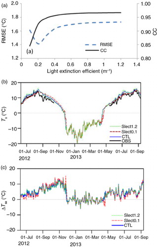
The results of SLCLM were very sensitive to Lec at its values <0.5m⁻¹, which value has been also estimated as a critical threshold for model response to the external forcing in previous lake modelling studies over low-elevation lakes (Heiskanen et al., 2015; Zolfaghari et al., 2016). At Lec higher than the critical value, no significant effect of Lec variation on simulations was present. At low Lec, in turn, because of the deeper penetration of solar radiation and less heat stored in the lake layer close to water surface, the simulated T _s during the lake heating period was lower than in observations (Fig. 5b). During lake cooling, after September, the simulated temperature decreased more slowly and was slightly higher than observed, because of a larger amount of heat accumulated previously in the lake. The effects of Lec on simulated T _s over Ngoring Lake were similar to the previous findings from lakes in other regions (Martynov et al., 2010; Thiery et al., 2014a; Heiskanen et al., 2015; Zolfaghari et al., 2016). In the whole range of Lec variability from 0.1m⁻¹ to 1.2m⁻¹, the lake surface heating was strong enough to maintain positive ΔT _sa throughout the ice-free period of Ngoring Lake (Fig. 5c).

6. Effects of local climate

6.1. Configuration of the sensitivity experiments

To investigate effects of high-altitude climatic conditions on the positive difference between the lake surface temperature T _s and the air temperature T _a, following numerical experiments were performed with each atmospheric characteristics varying to imitate a low-elevation climate (mostly based on the values reported from Taihu Lake basin, which is located at a similar latitude as Ngoring Lake at the altitude of 3m asl):

• Sta: Increasing T _a by 6.5 °C to approximate the effect of higher T _a caused by the drop of 1000m altitude according to the overall environment adiabatic rate.

• Sswd: Reducing Swd by 35 % based on the annual mean solar radiation ratio between Taihu Lake basin and the Ngoring Lake basin (R _T/L=0.65) based on data from the Institute of Tibetan Plateau Research, Chinese Academy of Sciences (Chen et al., 2011).

• Slwd: 1.6 times increase of Lwd, according to the calculated ratio R _T/L.

• Sq: Setting forcing q as the maximum of the saturated specific humidity or 2.8 times (the calculated ratio R _T/L of specific humidity) the observed specific humidity.

• Sws: Reducing ws by 20 % according to the ratio R _T/L=0.8 for ws.

• Sps: 1.6 times increase of ps based on the ratio between sea level and Ngoring Lake basin.

• S(variable)±20 % (2 %): Forcing variables (Swd, Lwd, q, ws, ps and T _a) are increased or decreased by 20 or 2 %.

The above scenarios are quite artificial, because the atmospheric variables are closely interrelated. Still, the sensitivity studies in this formulation are able to shed a light on the major factors governing the air–lake interaction in high-altitude conditions.

6.2. Effects of T_a

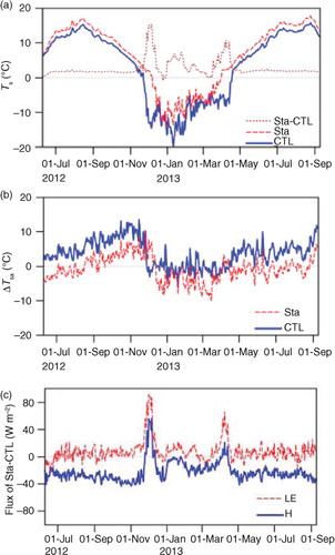
The 6.5 °C raise of T _a produced ~2.5 °C increase of T _s in Sta (Fig. 6a) during the ice-free period in both CTL and Sta (Fig. 6a) and shortened the ice-covered period, compared with CTL. When ice cover appeared in CTL and did not appear in Sta, the greatest T _s difference between CTL and Sta occurred reaching 16 °C. ΔT _sa in Sta was smaller in magnitude than in CTL and was predominately negative (characteristic of a stable boundary layer) before September in 2012 and 2013 (Fig. 6b). Hence, the cold air temperature over TP has the major contribution toward formation of the boundary layer instability over unfrozen Ngoring Lake in spring and summer. H decreased in accordance with the reduced ΔT _sa (Fig. 6c). In turn, LE increased because of increased saturated vapour pressure of the air at higher T _a resulting in a greater water loss from the lake surface (Fig. 6c).

Fig. 6 (a) Simulated T _s in CTL (blue solid line) and the sensitivity experiment Sta (red dashed line) and simulated T _s difference (brown dotted line) between CTL and Sta, (b) simulated ΔT _sa in CTL (blue solid line) and Sta (red dashed line), and (c) simulated H (blue solid line) and LE (red dashed line) difference between CTL and Sta.

6.3. Effects of solar radiation

With 40 % decrease in solar radiation in Sswd, the lake surface became colder and began to freeze 15d earlier than in CTL (Fig. 7a). The ice in the CTL melt up in the middle of April 2013, but the ice still existed until the end of May and melt 39d later in Sswd. The T _s difference between Sswd and CTL was about −4 °C during the ice-free period and was the largest (about −15 °C) when ice appeared in Sswd, and there was no ice in CTL. The positive ΔT _sa during the ice-free period in CTL was reduced in Sswd (Fig. 7b), turning occasionally negative during May–August. The reduced solar radiation shortened periods of instability (postive ΔT _sa) over ice-free lake and shifted dates of their first appearance from May to July. Hence, the strong radiative heating of Ngoring Lake is, along with the low air temperatures, a major factor affecting formation of the unstable boundary layer over the lake. Although the effect of the changed solar radiation in Sswd (reducing Swd to imitate the sea level condition) was quantitatively weaker than the effect of the changed air temperature in Sta (increasing T _a by 6.5 °C to approximate the drop of 1000m altitude), the two factors are strongly interrelated, both being characteristic at high altitudes.

Fig. 7 Same as Fig. 6, but for CTL and the sensitivity experiment Sswd.

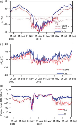
The decrease of the incoming solar radiation also reduced the surface heat fluxes H and LE (Fig. 7c). In open-water periods, the decrease of LE was about 30Wm⁻² stronger than the decrease of H, whereas in ice-covered periods, they were nearly equal, that is, the changed T _s resulting from the decreased solar radiation had a greater influence on the saturated vapour pressure and LE than on the sensible heat exchange H.

6.4. Effects of downward longwave radiation

With the 60 % increased annual mean incoming Lwd, T _s in the open-water lake increased by about 6 °C (Fig. 8a). The ice-covered period decreased from 147d in the CTL to 40d in Slwd. At the same time, T _s increased during in ice-free period, making ΔT _sa always positive over Ngoring Lake and higher than in CTL (Fig. 8b). Hence, in a very hypothetical case of the Lwd increase without any increase of the air temperature, the instability of the air–lake boundary layer would be stronger by increase of radiative heating of the lake surface.

Fig. 8 Same as Fig. 6, but for CTL and the sensitivity experiment Slwd.

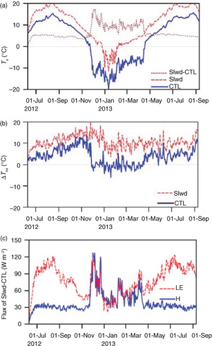
Compared with the CTL, increased Lwd and T _s in the Slwd experiment induced about 35Wm⁻² increase in H and maintained the heat transfer from the lake surface to the atmosphere throughout the simulated period. The increased Lwd and T _s induced a stronger increase in LE (50–120Wm⁻²) than H (35Wm⁻²) (Fig. 8c) during the ice-free period mainly owing to significant effects of the changed lake surface temperature on saturated vapour pressure, similarly as in Sswd (see also Section 6.3).

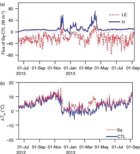
6.5. Effects of air humidity

A more humid air reduces the difference between the specific humidity and the saturated value that suppresses evaporation. Compared with CTL, LE in Sq was reduced by up to 80Wm⁻² with strong short-term variations, whereas H increased by approximately 15Wm⁻² over the period without ice cover (Fig. 9a). Owing to the weaker heat loss in Sq, the lake became slightly warmer (figure not shown). Thus, ΔT _sa was increased by about 2 °C over ice-free period (Fig. 9b). Comparing CTL and Sq, the relatively low specific humidity on TP had the negative effects on the observed positive ΔT _sa over Ngoring Lake.

Fig. 9 (a) Simulated H (blue solid line) and LE (red dashed line) difference between CTL and the sensitivity experiment Sq, and (b) simulated ΔT _sa in CTL (blue solid line) and Sq (red dashed line).

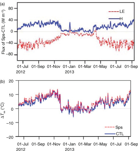
6.6. Effects of air pressure

The increased air pressure would increase air density and H in Sps, but it also could reduce the saturated specific humidity with the same specific humidity at the same temperature and suppress evaporation. The LE in Sps was reduced by less than 60Wm⁻², and H increased by less than 40Wm⁻² (Fig. 10a). The additional energy was stored in the lake, increasing ΔT _sa and T _s by about 2 °C in the ice-free period (Fig. 10a). The ps change did not cause any change of the ice-covered period. The low pressure in TP had little effect on positive ΔT _sa during the lake ice-free period.

Fig. 10 Same as Fig. 9, but for CTL and the sensitivity experiment Sps.

6.7. Effects of ws

Compared with CTL, the weakened wind in Sws suppressed evaporation and made lake warmer and increased H. However, the change was very small in Sws (figure not shown) and could be neglected compared to other experiments, similar to the results found in Taihu (Gu et al., 2013).

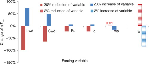
6.8. Sensitivity of ΔT _sa to each forcing factor

The sensitivity of simulated annual mean ΔT _sa (from July 2012 to June 2013) to each forcing variable was obtained with 20 % (for Swd, Lwd, q, ps and ws) or 2 % (for T _a) change of variables based on CTL. ws and T _a were negatively correlated with ΔT _sa, while changes in the other variables had positive effects (Fig. 11). The simulated results were the most sensitive to changes in T _a, followed by Lwd, Swd, q, ws and ps.

Fig. 11 Changed percentage of annual mean ΔT _sa from July 2012 to June 2013 in each simulation experiment (with percentage change of each variable) compared to that of CTL.

7. Discussion and conclusions

The mostly positive ΔT _sa over an open-water lake at high altitude on the TP was investigated based on observations and the one-dimensional lake model SLCLM. Three-year data consisting of three types of observations, including T _s calculated from upward longwave radiation, and directly observed T _w and H, showed that the surface and top layers of Ngoring Lake (4280m asl) were warmer than T _a without ice cover from spring to early winter. ΔT _sa over Ngoring Lake had two peaks of positive ΔT _sa in May and November and the lowest value in June. A similar phenomenon of surface unstable layer appeared in other lakes of TP: The Yamdrok Lake (28.26–29.18°N, 90.35–91.08°E, 4441.5m asl), with a similar altitude to Ngoring Lake (4200m), had a monthly mean temperature pattern very similar to Ngoring Lake (Yu et al., 2011). The monthly mean temperature difference peaked in November when the monthly H was the highest. The phenomenon with the higher daily mean T _s compared with T _a was also observed over a small lake next to the large Nam Co Lake in the observation period from April to September 2012 (Wang et al., 2015).

Among lakes in other regions of the world, the lake surface persistently warmer than the air was observed in tropical and subtropical lakes. In Lake Tanganyika (3–9°N, 29–31°E, maximum depth 1470m; 32 600km²), the lake water is generally warmer than the air, and the highest monthly percentage of stable conditions was only 6 % (Verburg and Antenucci, 2010). The 7-d moving average air–lake temperature difference varied within 3 °C range. The peak appeared in the middle of the wet warm season (May–September) of the tropical region and was smaller than that over Ngoring Lake. In Taihu Lake (31.4°N, 120.22°E, 1.9m deep), located in a subtropical region, the seasonal variations of T _w and T _a were qualitatively similar to those over Ngoring Lake, while never dropped below 0 °C, and no ice cover was formed. ΔT _sa over Taihu Lake was always positive throughout the year, with weak seasonal variations and the magnitude <2 °C (Wang et al., 2014), indicating much weaker boundary layer instability than that observed over Ngoring Lake.

Similar to Ngoring Lake, ΔT _sa over the Great Slave Lake (61.6°N, 114.0°E, 160m asl, maximum depth 614m, mean depth 41m) increased during the open-water period and reached the highest values during the cooling season in autumn and early winter. However, the boundary layer remained stable during the warming season, with temperature difference changing the sign from negative to positive in August, typical for temperate lakes (Long et al., 2007; Rouse et al., 2008) and different with the almost persistent positive ΔT _sa over Ngoring Lake starting from the ice break-up in late spring. In the medium-sized salt lake, Thau Lagoon (43.4°N, 3.6°E), located at the French coast of the Mediterranean Sea, the T _w and T _a reached the highest values around August and the lowest (above 0 °C) in January, similarly to the seasonal pattern of Ngoring Lake. The water was warmer than the air from April to November, but the temperature difference did not increase during the months close to November, in contrast to Ngoring Lake (Bouin et al., 2012).

In summary, both T _w and T _s of Ngoring Lake were higher than T _a during the open-water period, similar to the situation in tropical and subtropical lakes and different from temperate and boreal lakes at low altitudes. On the contrary, ΔT _sa over Ngoring Lake increased from late spring to late autumn, following the seasonal pattern similar to that of low-altitude temperate lakes (Kirillin, 2010), but different from tropical lakes (Verburg and Antenucci, 2010).

Apart from the TP, a similar unstable temperature difference pattern was observed over alpine lake La Caldera (37°N, 3.3°W, 3050m asl) from early July to August (Rueda et al., 2007), suggesting the boundary layer instability to be a common phenomenon for high-altitude lakes. The SLCLM demonstrated good performance for high-altitude lakes, although originally developed based on low-altitude lakes. The simulated results, including ΔT _sa, were close to the observations.

A series of sensitivity simulations with SLCLM demonstrated that lake depth, lake water surface albedo and light extinction coefficient Lec had little effect on the sign of positive ΔT _sa over the TP lakes during the ice-free period. The simulations showed that changes in the lake depth from 2 to 32m could affect the magnitude of ΔT _sa but could not change the direction of heat transfer. Different lake surface albedo values including the observed lake water albedo did not have significant effects on the simulation. Higher water transparency with deeper penetration of solar radiation could cool the lake surface and decrease ΔT _sa during the period from ice melting to the month with the highest T _a, and vice versa when temperature dropped. With the higher water transparency (0.1m⁻¹ Lec), the positive ΔT _sa was also simulated over Ngoring Lake during ice-free period.

Sensitivity tests imitating the conditions over the lowland basin of Taihu Lake, with a close latitude and the altitude of only 3m asl, showed that the main contributors of local climate characteristics to the positive ΔT _sa are the low T _a and the strong solar radiation caused by high altitude. Increasing T _a by 6.5 °C with about 1000 m altitude dropping and reducing 35 % solar radiation to close to the Taihu Lake basin would both change the sign of ΔT _sa in spring and early summer and maintain the positive values only in autumn. Compared with characteristics of Taihu Lake basin with the similar latitude and sea surface level, low Lwd, small q, low ps and strong winds in TP would cool down the surface. The simulated results are the most sensitive to the change of T _a, then Lwd, and the least to the change of ws.

8. Acknowledgments

The study was supported by the National Natural Science Foundation of China (91637107, 41475011, 41275014, 41605011 and 41375019). We acknowledge the support for using the computing resources at the Supercomputing Center of Cold and Arid Regions Environmental and Engineering Research Institute, Chinese Academy of Sciences. GK was supported by the German Science Foundation (DFG project KI 853/11–1). Comments and suggestions of two anonymous reviewers have helped to improve the quality of the original manuscript.

References

- Biermann T. , Babel W. , Ma W. , Chen X. , Thiem E. , co-authors . Turbulent flux observations and modelling over a shallow lake and a wet grassland in the Nam Co basin, Tibetan Plateau. Theor. Appl. Climatol. 2014; 116: 301–316.
- Bouin M. N., Caniaux G., Traulle O., Legain D., Le Moigne P. Long-term heat exchanges over a Mediterranean lagoon. J. Geophys. Res. 2012; 117: 23104. http://dx.doi.org/10.1029/2012jd017857.
- Cao C. , Lee X. , Zhang M. , Liu S. , Xiao W. , co-authors . Temporal and spatial characteristics of lake Taihu surface albedo and its impact factors. Environ. Sci. 2015; 36: 3611–3619. in Chinese with English abstract.
- Chen Y. Y., Yang K., He J., Qin J., Shi J. C., co-authors. Improving land surface temperature modeling for dry land of China. J. Geophys. Res. 2011; 116: 20104. http://dx.doi.org/10.1029/2011jd015921.
- Elo P. A. R . The energy balance and vertical thermal structure of two small boreal lakes in summer. Boreal Environ. Res. 2007; 12: 585–600.
- Fairall C. W. , Bradley E. F. , Godfrey J. S. , Wick G. A. , Edson J. B. , Young G. S . Cool-skin and warm-layer effects on sea surface temperature. J. Geophys. Res. 1996; 101: 1295–1308.
- Fang X. , Stefan H. G . Long-term lake water temperature and ice cover simulations/measurements. Cold. Reg. Sci. Technol. 1996; 24: 289–304.
- Gu H. , Shen X. , Jin J. , Xiao W. , Wang Y . An application of a 1-D thermal diffusion lake model to Lake Taihu. Acta. Meteorol. Sin. 2013; 71: 719–730. in Chinese with English abstract.
- Haginoya S. , Fujii H. , Kuwagata T. , Xu J. Q. , Ishigooka Y. , co-authors . Air-lake interaction features found in heat and water exchanges over Nam Co on the Tibetan Plateau. Sola. 2009; 5: 172–175.
- Heiskanen J. J., Mammarella I., Ojala A., Stepanenko V., Erkkilä K.-M., co-authors. Effects of water clarity on lake stratification and lake-atmosphere heat exchange. J. Geophys. Res. 2015; 120: 7412–7428. http://dx.doi.org/10.1002/2014jd022938.
- Hostetler S. W. , Bates G. T. , Giorgi F . Interactive coupling of a lake thermal model with a regional climate model. J. Geophys. Res. 1993; 98: 5045–5057.
- Ji G. , Jiang H. , Lu L . Characteristics of longwave radiation over the Qinghai-Xizang Plateau. Plateau. Meteorol. 1995; 14: 451–458. in Chinese with English abstract.
- Jiang J. , Huang Q . Distribution and variation of lakes in Tibetan Plateau and their comparison with lakes in other part of China. Water. Res. Prot. 2004; 4: 24–27. in Chinese with English Abstract.
- Kirillin G . Modeling the impact of global warming on water temperature and seasonal mixing regimes in small temperate lakes. Boreal. Environ. Res. 2010; 15: 279–293.
- Li M. , Ma Y. , Hu Z. , Ishikawa H. , Oku Y . Snow distribution over the Namco lake area of the Tibetan Plateau. Hydrol. Earth. Syst. Sci. 2009; 13: 2023–2030.
- Li Z. , Lyu S. , Ao Y. , Wen L. , Zhao L. , co-authors . Long-term energy flux and radiation balance observations over Lake Ngoring, Tibetan Plateau. Atmos. Res. 2015; 155: 13–25.
- Long Z. , Perrie W. , Gyakum J. , Caya D. , Laprise R . Northern lake impacts on local seasonal climate. J. Hydrometeorol. 2007; 8: 881–896.
- Martynov A. , Sushama L. , Laprise R . Simulation of temperate freezing lakes by one-dimensional lake models: performance assessment for interactive coupling with regional climate models. Boreal. Environ. Res. 2010; 15: 143–164.
- Mironov D. , Heise E. , Kourzeneva E. , Ritter B. , Schneider N. , co-authors . Implementation of the lake parameterisation scheme FLake into the numerical weather prediction model COSMO. Boreal. Environ. Res. 2010; 15: 218–230.
- Nordbo A., Launiainen S., Mammarella I., Lepparanta M., Huotari J., co-authors. Long-term energy flux measurements and energy balance over a small boreal lake using eddy covariance technique. J. Geophys. Res. 2011; 116: 02119. http://dx.doi.org/10.1029/2010jd014542.
- Oleson K. W. , Lawrence D. M. , Bonan G. B. , Flanner M. G. , Kluzek E. , co-authors . Technical Description of Version 4.0 of the Community Land Model. 2010; Boulder, MA: NCAR.
- Oleson K. W. , Lawrence D. M. , Bonan G. B. , Flanner M. G. , Kluzek E. , co-authors . Technical Description of Version 4.5 of the Community Land Model. 2013; Boulder, MA: NCAR.
- Rouse W. R., Blanken P. D., Bussieres N., Oswald C. J., Schertzer W. M., co-authors. Investigation of the thermal and energy balance regimes of Great Slave and Great Bear Lakes. J. Hydrometeorol. 2008; 9: 1318–1333. http://dx.doi.org/10.1175/2008jhm977.1.
- Rueda F., Moreno-Ostos E., Cruz-Pizarro L. Spatial and temporal scales of transport during the cooling phase of the ice-free period in a small high-mountain lake. Aquat. Sci. 2007; 69: 115–128. http://dx.doi.org/10.1007/s00027-006-0823-8.
- Stepanenko V. , Jöhnk K. D. , Machulskaya E. , Perroud M. , Subin Z. , co-authors . Simulation of surface energy fluxes and stratification of a small boreal lake by a set of one-dimensional models. Tellus A. 2014; 66: 174–179.
- Stepanenko V. M. , Goyette S. , Martynov A. , Perroud M. , Fang X. , co-authors . First steps of a Lake model intercomparison project: LakeMIP. Boreal. Environ. Res. 2010; 15: 191–202.
- Subin Z. M., Riley W. J., Mironov D. An improved lake model for climate simulations: model structure, evaluation, and sensitivity analyses in CESM1. J. Adv. Mod. Earth. Sys. 2012; 4: 02001. http://dx.doi.org/10.1029/2011ms000072.
- Thiery W., Martynov A., Darchambeau F., Descy J. P., Plisnier P. D., co-authors. Understanding the performance of the FLake model over two African Great Lakes. Geosci. Model. Dev. 2014a; 7: 317–337. http://dx.doi.org/10.5194/gmd-7-317-2014.
- Thiery W. , Stepanenko V. M. , Fang X. , Jöhnk K. D. , Li Z. , co-authors . LakeMIP Kivu: evaluating the representation of a large, deep tropical lake by a set of one-dimensional lake models. Tellus A. 2014b; 66: 1–18.
- Verburg P., Antenucci J. P. Persistent unstable atmospheric boundary layer enhances sensible and latent heat loss in a tropical great lake: Lake Tanganyika. J. Geophys. Res. 2010; 115 http://dx.doi.org/10.1029/2009JD012839.
- Wang B., Ma Y., Chen X., Ma W., Su Z., co-authors. Observation and simulation of lake-air heat and water transfer processes in a high-altitude shallow lake on the Tibetan Plateau. J. Geophys. Res. 2015; 120: 12327–12344. http://dx.doi.org/10.1002/2015jd023863.
- Wang J. , Peng P. , Ma Q. , Zhu L . Modern limnological features of Tangra Yumco and Zhari Namco, TibetanPlateau (in Chinese with English abstract). J. Lake. Sci. 2010; 22: 629–632.
- Wang W. , Xiao W. , Cao C. , Gao Z. , Hu Z , co-authors . Temporal and spatial variations in radiation and energy balance across a large freshwater lake in China. J. Hydrol. 2014; 511: 811–824.
- Wen L., Lv S., Li Z., Zhao L., Nagabhatla N. Impacts of the two biggest lakes on local temperature and precipitation in the Yellow River source region of the Tibetan Plateau. Adv. Meteorol 2015. 2015; 10. http://dx.doi.org/10.1155/2015/248031.
- Xiao W. , Liu S. D. , Wang W. , Yang D. , Xu J. P. , co-authors . Transfer coefficients of momentum, heat and water vapour in the atmospheric surface layer of a large freshwater lake. Bound-lay. Meteorol. 2013; 148: 479–494.
- Xu Y. , Kang S. , Zhang Y. , Zhang Y . A method for estimating the contribution of evaporative vapor from Nam Co to local atmospheric vapor based on stable isotopes of water bodies. Chinese Sci. Bull. 2011; 56: 1511–1517.
- Yu S. , Liu J. , Xu J. , Wang H . Evaporation and energy balance estimates over a large inland lake in the Tibet-Himalaya. Environ. Earth. Sci. 2011; 64: 1169–1176.
- Zhang G. , Yao T. , Xie H. , Zhang K. , Zhu F . Lakes’ state and abundance across the Tibetan Plateau. Chinese Sci. Bull. 2014; 59: 3010–3021.
- Zolfaghari K., Duguay C. R., Kheyrollah Pour H. Satellite-derived light extinction coefficient and its impact on thermal structure simulations in a 1-D lake model. Hydrol. Earth. Syst. Sci. Discuss. 2016; 2016: 1–36. http://dx.doi.org/10.5194/hess-2016-82.