
Abstract
In this paper, two important issues are raised for multistep variational data assimilation in which broadly distributed coarse-resolution observations are analysed in the first step, and then locally distributed high-resolution observations are analysed in the second step (and subsequent steps if any). The first one concerns how to objectively estimate or efficiently compute the analysis error covariance for the analysed field obtained in the first step and used to update the background field in the next step. To attack this issue, spectral formulations are derived for efficiently calculating the analysis error covariance functions. The calculated analysis error covariance functions are verified against their respective benchmarks for one- and two-dimensional cases and shown to be very (or fairly) good approximations for uniformly (or non-uniformly) distributed coarse-resolution observations. The second issue concerns whether and under what conditions the above calculated analysis error covariance can make the two-step analysis more accurate than the conventional single-step analysis. To answer this question, idealised numerical experiments are performed to compare the two-step analyses with their respective counterpart single-step analyses while the background error covariance is assumed to be exactly known in the first step but the number of iterations performed by the minimisation algorithm is limited (to mimic the computationally constrained situations in operational data assimilation). The results show that the two-step analysis is significantly more accurate than the single-step analysis until the iteration number becomes so large that the single-step analysis can reach the final convergence or nearly so. The two-step analysis converges much faster and thus is more efficient than the single-step analysis to reach the same accuracy. Its computational efficiency can be further enhanced by properly coarsening the grid resolution in the first step with the high-resolution grid used only over the nested domain in the second step.
1. Introduction
It has been well recognised that using a Gaussian function with a synoptic-scale de-correlation length to model the background error covariance in data assimilation can inadvertently hamper the ability of the analysis to assimilate mesoscale structures. As a remedy to this problem, a superposition of Gaussians has been formulated (Purser et al., Citation2003), and double Gaussians have been used to model the background error correlation in variational data assimilation at National Centers of Environmental Prediction (NCEP) with increased computational cost (Wu et al., Citation2002), but the mesoscale features are still overly smoothed and inadequately resolved in the analysed incremental fields even in areas covered by remotely sensed high-resolution observations, such as those from operational weather radars (Liu et al., Citation2005). This raises an important question on how to optimally assimilate patchy high-resolution observations, such as those remotely sensed from radars and satellites, along-side sparse observations into a high-resolution model.
Ideally and theoretically, if the background error covariance is exactly known and perfectly modelled in data assimilation, then all different types of observations can be optimally analysed in a single batch. Such a single-step approach has been widely adopted in operational variational data assimilation. However, since the background error covariance is largely unknown and often crudely modelled, the analysis is not truly optimal. Furthermore, even if the background error covariance is accurately modelled (for idealised cases such as those to be presented in this paper), the analysis obtained by a minimisation algorithm is still not optimal unless the minimisation is performed thoroughly with a sufficiently large number of iterations to reach the true global minimum of the cost-function. In operational variational data assimilation, the number of iterations is limited by the computational constraints and often far from sufficient due to the extremely large dimension of the minimisation problem, and as a result, the analysis could be far from optimal. This speculation can be more or less supported by the recent study of CitationLi et al. (2015) in which double Gaussians were also used to model the background error correlation but the cost-function was truly minimised in their idealised experiments. In particular, the double Gaussians were found to be quite effective in assimilating patchy high-resolution observations along-side sparse observations although the true background error correlation was not exactly modelled by the double Gaussians in either of their multiscale variational schemes (AB-DA and MS-DA). In view of the aforementioned limitations in operational data assimilation and inspired by the study of CitationLi et al. (2015), we are motivated to explore new multiscale and multistep approaches that can be not only more effective and accurate but also more efficient than the single-step approach for assimilating different types of observations with distinctively different spatial resolutions and distributions (including remotely sensed high-resolution observations).
Previously, CitationXie et al. (2011) proposed a sequential multistep variational analysis approach for a multiscale analysis system with observations reused in each step in a fashion similar to the Barnes successive correction scheme. They noted that the background error covariance should change with different steps to incorporate scale-dependent information (like the Barnes successive correction scheme) but left this issue to future studies for further improvements. CitationGao et al. (2013) adopted a real-time variational data assimilation system in which a two-step approach was employed to analyse observations of different spatial resolutions. In their two-step approach, a reduced background error de-correlation length was used in the second step, but the background error de-correlation length and error variances for different model variables were specified empirically in each step. This left the issue on how to objectively estimate the error covariance for the updated background largely unaddressed.
For the traditional single-step variational analysis, the background error covariance can be estimated from the time series of innovation (i.e. observation minus background in the observation space) by using the innovation method (Hollingsworth and Lonnberg, Citation1986; Lonnberg and Hollingsworth, Citation1986; Xu and Wei, Citation2001, Citation2002; Xu et al., Citation2001) or from the time series of difference between two model forecasts verified at the same time by using the National Meteorological Center (NMC) method (Parrish and Derber, Citation1992; Derber and Bouttier, Citation1999). The background error covariance estimated by the above method can be readily used for the variational analysis in the first step of a multistep approach. In each subsequent step, however, the background error covariance should be re-estimated for the updated background, that is, the analysis produced from the previous step. The innovation method can be modified and used for the re-estimation if the observations used in current step are not previously used and thus are new and independent of the new background and if the following two conditions are also satisfied (as required by the innovation method): (1) the time series of new innovation (that is, new observation minus new background) still satisfy the ergodicity assumption (and thus can be used as an ensemble), and (2) the statistic structures of the new innovations remain to be horizontally homogeneous and isotropic. These two conditions often cannot be satisfied, as they require that the distribution of the observations used in each step is not only horizontally homogeneous (or nearly so) but also largely fixed in the time series. Thus, the innovation method must be simplified with reduced conditions to re-estimate the new background error variance only. In particular, as shown in (9) of CitationXu et al. (2015), by using the local spatial mean (instead of temporal mean) as the ensemble mean, the background error variance can be estimated as a smooth function of space from the new innovation field (rather than an ensemble collected from a time series) in each step of a multistep approach. The background error de-correlation length, however, is still specified empirically in each step of the multistep radar wind analysis system of CitationXu et al. (2015). None of the studies cited above has adequately addressed or satisfactorily solved the problem on how to objectively estimate or efficiently compute the error covariance for the updated background. We believe that this issue is very important for a multistep variational approach because the analysis increment in each subsequent step is largely controlled by the error covariance of the updated background, while directly computing the error covariance [see eq. (1b)] is impractical for operational data assimilation.
In this study, a new approach is explored to efficiently but approximately calculate the analysis error covariance for multiscale and multistep variational data assimilation. For simplicity, we will consider only two types of observations with distinctively different spatial resolutions and distributions. The first type consists of coarse-resolution observations distributed over the entire analysis domain, while the second type consists of high-resolution observations densely distributed over a fraction of the analysis domain. A two-step variational method will be designed to analyse the coarse-resolution observations in the first step and then the high-resolution observations in the second step. As a new aspect of this two-step variational method, spectral formulations will be derived and simplified for efficiently calculating the analysis error covariance in the first step to update the background error covariance in the second step. The paper is organised as follows. The spectral formulations are derived in the next section after a brief review of the formulations for the optimally analysed state vector and associated error covariance. Using the spectral formulations, two-step variational analyses are performed versus single-step variational analyses for one-dimensional cases in Section 3 and for two-dimensional cases in Section 4 to support the speculation stated at the beginning of this section. Conclusions follow in Section 5.
2. Spectral formulations for efficiently estimating analysis error covariance
2.1. Review of formulations for optimal analysis
When the variational analysis is formulated optimally based on the Bayesian estimation theory (see Chapter 7 of Jazwinski, Citation1970), the background state vector b is updated to the analysis state vector a with the following analysis increment:1a
and the background error covariance matrix B is updated to the following analysis error covariance matrix:1b
where R is the observation error covariance matrix, H denotes the (linearised) observation operator, ( )T denotes the transpose of ( ), d=y− H (b) is the innovation vector (observation minus background in the observation space), y is the observation vector, H ( ) denotes the observation operator and H is the linearised H ( ).
Theoretically, for a linear observation operator H ( )=H, eq. (1b) provides a precise formulation for updating B to A in each subsequent step of a multistep variational analysis, but the required computational cost is impractical for operational applications. Thus, what we need here is to simplify eq. (1b) so that A can be calculated approximately with much reduced computational cost. This issue will be addressed in the next two subsections by transforming eq. (1b) into simplified spectral forms for coarse-resolution innovations in one- and two-dimensional spaces so that A can be very efficiently calculated with certain approximations.
As mentioned in the introduction, we will simply consider only two types of observations: (1) coarse-resolution observations either uniformly or non-uniformly distributed over the analysis domain, and (2) high-resolution observations over a fraction of the analysis domain. The coarse-resolution observations are analysed in the first step over the entire domain. The high-resolution observations are then analysed in the second step over a nested domain with the background state b updated by a obtained from the first step and the background error covariance B updated by the approximately calculated A using the spectral formulation. After this, the next important question is whether and how the approximately calculated A can make the two-step analysis more accurate than the single-step analysis of the coarse-resolution and high-resolution observations together if the number of iterations is not sufficiently large and thus neither analysis can be optimal (as explained in Section 1). This question will be answered in Section 3 for one-dimensional cases and in Section 4 for two-dimensional cases.
2.2. Spectral formulations for one-dimensional case
Consider that there are M coarse-resolution observations uniformly spaced every Δx
co over a one-dimensional analysis domain of length D=MΔx
co=NΔx, where N is the number of analysis grid points and Δx is the grid spacing. By periodically extending D in x for the random fields of observation error and background error, eq. (1b) can be transformed into the following spectral form in the wavenumber space:2
where S a ≡ F N AF N H, ( )H denotes the Hermitian transpose of ( ), S ≡ F N BF N H (or C ≡ F M RF M H) is a diagonal matrix in R N (or R M ), F N (or F M ) is the normalised discrete Fourier transformation (DFT) matrix in R N (or R M ), ν=N/M=Δx co/Δx (>1), Π=P MN SP MN T is a diagonal matrix in R M for N>M, and P MN is a M×N matrix given by (19) of CitationXu (2011). When ν happens to be an odd integer, P MN is simply given by (I M , …, I M ) where I M is the unit matrix in R M . The spectral formulations in Section 2.2 of CitationXu (2011) are used in deriving eq. (2) and above results.
As M<N, S
a is not diagonal, but its non-zero off-diagonal elements are sparse and negligibly small. Using eq. (2), the diagonal part of S
a can be very efficiently calculated from S and C, as shown in the Appendix. The diagonal part of S
a can then be transformed also very efficiently by the inverse DFT back to the physical space in the form of σ
e
2
C
a(x
i
– x
j
) to give the ijth element of A, where σ
e
2 (=constant) and C
a(x) denote the approximately calculated analysis error variance and correlation function, respectively. In this case, as the analysis error power spectrum associated with the approximately calculated A is given by the diagonal part of S
a in the discrete form of S
a
(k
i
), where k
i
=iΔk is the ith discrete wave number and Δk≡2π/D is the minimum resolvable wavenumber, the analysis error covariance can be also obtained approximately in the following continuous form:3
where q i =1 for 1≤i<N q , q i =½ for i=0 and i=N q ≡Int[(N+1)/2]≥N +≡Int[N/2], and Int[ ] denotes the integer part of [ ]. The derivation of eq. (3) is similar to that in (17) of CitationXu (2011) but applied to the inverse Fourier transformation of S a (k i ) with C a(x) obtained by the ideal trigonometric polynomial interpolation. When the M coarse-resolution observations are not uniformly spaced over the analysis domain, the above formulations still can be used to calculate A approximately (see Sections 3.3 and 3.4).
2.3. Spectral formulations for two-dimensional case
Now, we consider that there are M=M x M y coarse-resolution observations uniformly spaced by Δx co along the x direction and Δy co along the y direction in a two-dimensional analysis domain of length D x =M x Δx co=N x Δx and width M y Δy co=D y =N y Δy, where N x (or N y ) is the number of analysis grid points and Δx (or Δy) is the grid spacing along the x (or y) direction in the analysis domain. In this case, by periodically extending D x in x and D y in y for the random fields of observation error and background error, eq. (1b) can be transformed into the same spectral form as in eq. (2), except that F N =F Nx ⊗F Ny (or F M =F Mx ⊗F My ) is now the tensor product of the two normalised DFT matrices F Nx and F Ny (or F Mx and F My ) with N=N x N y (or M=M x M y ), ν = ν x ν y , ν x =N x /M x =Δx co/Δx (>1), ν y = N y /M y =Δy co/Δy (>1), and P MN =P MxNx ⊗P MyNy is a M×N matrix with P MxNx and P MyNy given in the same way as described for the one-dimensional case in eq. (2). The spectral formulations in Section 2.3 of CitationXu (2011) are used in deriving the two-dimensional spectral form of eq. (2) and the above results.
Again, as M<N, S
a is not diagonal but its non-zero off-diagonal elements are sparse and negligibly small. Using the two-dimensional spectral form of eq. (2), S
a can be easily calculated from S and C (see the Appendix). The diagonal part of S
a can be then transformed efficiently back to the physical space in the form of σ
e
2
C
a(x
i
–x
j
) to give the ijth element of A, where x ≡ (x, y), σ
e
2 and C
a(x) denote the approximately calculated analysis error variance and correlation function, respectively. Now the diagonal part of S
a has the discrete form of S
a
(k
i
, k
j
) where k
i
=iΔk
x
(or k
y
=jΔk
y
) is the ith (or i'th) discrete wavenumber in k
x
(or k
y
) and Δk
x
≡2π/D
x
(or Δk
y
≡2π/D
y
) is the minimum resolvable wavenumber in the x (or y) direction. From S
a
(k
i
, k
j
), the analysis error covariance can be also obtained approximately in the following continuous form:4
where q i (or q j )=1 for 1≤i (or j)<N qx (or N qy ), q i (or q j )=½ for i (or j)=0 and for i=N qx (or j=N qy ), N qx ≡Int[(N x +1)/2]≥N +x ≡Int[N x /2], and N qy ≡Int[(N y +1)/2]≥N +y ≡Int[N y /2]. The derivation of eq. (4) is similar to that of eq. (3) but extended for the two-dimensional case. When the M coarse-resolution observations are not uniformly spaced in the x- and y-directions over the entire analysis domain, the two-dimensional spectral form of eqs. (2) and (4) remain approximately applicable (see Section 4.3).
3. Numerical experiments for one-dimensional cases
3.1. Descriptions of data and experiments
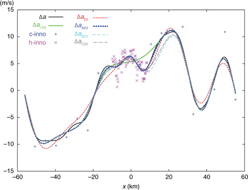
In this section, one-dimensional experiments are performed by using observations from the same data source (i.e. the radial velocities scanned by the NSSL phased array Doppler radar for the Oklahoma squall line on 2 June 2004) with the same model-produced background field as those described in Section 5.2 of Xu (Citation2007) and Section 3.1 of CitationXu and Wei (2011) except for the following treatments: (1) The analysis domain size is set to D=NΔx=110.4 km with N=23×20=460 and Δx=0.24 km, where Δx is the analysis grid resolution and is set to be the same as the original radar radial-velocity observation resolution. (2) The coarse-resolution innovations are produced by subtracting the background values from the original observations interpolated at M (=20) observational points that are uniformly (or non-uniformly) thinned from the original 460 observation points with the observation resolution coarsened exactly (or roughly) to Δx co=23Δx over the entire domain of length D as shown by the blue+signs in (or ), while the high-resolution innovations are obtained by subtracting the background values from the remaining original observations at M′ (= 73) observational points in a nested domain of length D/6 as shown by the purple × signs in Fig. 1 (or ).
Fig. 1 Uniformly distributed coarse-resolution innovations (c-inno) plotted by blue+signs, and high-resolution innovations (h-inno) plotted by purple x signs. The solid black curve plots the benchmark analysis increment Δa. The dashed red curve plots the analysis increment Δa 20 from SE with 20 iterations. The solid green curve plots the analysis increment Δa I-20 from the first step of two-step experiment (TEA, TEB or TEC) with 20 iterations. The dashed blue, dotted cyan and dot-dashed grey curves plot the analysis increments Δa A20 from TEA, Δa B20 from TEB and Δa C20 from TEC, respectively, with 20 iterations.
The observational and background errors are assumed to be Gaussian random and homogeneous over the analysis domain. The difference of these two errors is represented by the innovation. The innovation is thus also Gaussian random and homogeneous, and so does the analysis increment. This implies that the innovation and analysis increment fields can be extended periodically beyond the analysis domain, so the spectral formulations derived in the previous section can be used without actually extending the observation and background fields periodically beyond the analysis domain. As will be explained later and shown in Subsection 3.4 and Section 4, the spectral formulations can be also used without periodically extending the innovation and analysis increment fields.
The observation error variance is set to the estimated value of σ
o
2=2.52 m2s−2, as in Section 5.2 of Xu (Citation2007), while the background error variance is estimated by σ
b
2=σ
d
2−σ
o
2=25 m2s−2, where σ
d
2 is the innovation variance estimated by the spatially averaged value of squared innovations. The background error correlation function is modelled by the following double Gaussians:5
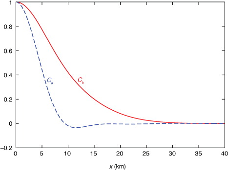
with L=10 km (=41.67Δx). This correlation function mimics the operationally used double Gaussians (see Sections 2 and 4 of Wu et al., Citation2002). When the analysis domain is extended periodically, the error correlation function is also extended periodically and this is done for each Gaussian function in the same way as shown in eq. (1b) of CitationXu and Wei (2011). The structure of C b(x) is shown by the solid red curve in . Note that D >> L and C b(x) becomes negligibly small as ∣x∣>3L (≈ 125Δx), so C b(x) is virtually not affected by the periodic extension over the primary period of −D/2<x<D/2. Thus, with the innovations extended periodically beyond the analysis domain, the analysis can be performed over the analysis domain by using only those innovations that are located within the extended domain of −D/2−3L≤x≤D/2+3L.
Fig. 2 C b(x) plotted by red curve and C a(x) plotted by dotted blue curve.
The background error power spectrum can be obtained from the periodically extended σ
b
2
C
b(x) by the DFT over D in the discrete form of S(k
i
), where S(k
i
) denotes the ith diagonal element of S [see (12)-(13) of Xu, Citation2011]. For the double-Gaussian form of C
b(x) in eq. (5), S(k
i
) can be also derived analytically [in the same way as for the single Gaussian form in eqs. (10)–(11) of Xu and Wei, Citation2011] in the following form:6
where A 1=Σ i exp[−(iD)2/(2L 2)]≈1 and A 2=Σ i exp[−2(iD)2/L 2]≈1 for D>>L. The discrete power spectrum S(k i ) is shown by the red+signs in . In the limit of N→∞ (or D→∞ with fixed Δx), Δk≡2π/D→0 and S(k i ) approaches its continuous counterpart S(k) plotted by the red curve in . As shown in , S(k i ) [or S(k)] decreases rapidly and becomes negligibly small as ∣k i ∣ (or ∣k∣) increases to and beyond 10Δk=5.7×10⁻⁴ m−1 but within N -Δk≤k i ≤N+Δk (or −π/Δx<k≤π/Δx) where N −≡Int[(1−N)/2].
Fig. 3 Discrete background error power spectrum S(k i ) (that forms the diagonal matrix S) plotted by red+signs, and discrete analysis error power spectrum S a(k i ) (that forms the diagonal part of S a) plotted by green×signs, where k i =iΔk and Δk≡2π/D=5.7×10−5 m−1. The solid red (or green) curve plots S(k) [or S a(k)], that is, the continuous counterpart of S(k i ) [or S a(k i )] in the limit of D=NΔx→∞ for fixed Δx.
![Fig. 3 Discrete background error power spectrum S(k i ) (that forms the diagonal matrix S) plotted by red+signs, and discrete analysis error power spectrum S a(k i ) (that forms the diagonal part of S a) plotted by green×signs, where k i =iΔk and Δk≡2π/D=5.7×10−5 m−1. The solid red (or green) curve plots S(k) [or S a(k)], that is, the continuous counterpart of S(k i ) [or S a(k i )] in the limit of D=NΔx→∞ for fixed Δx.](/cms/asset/a2273cdf-262f-4ed5-85ab-a967b97cef69/zela_a_11830317_f0003_ob.jpg)
Two sets of innovations are generated for the one-dimensional experiments in this section. Both sets consist of M coarse-resolution innovations and M′ high-resolution innovations. The coarse-resolution innovations are distributed uniformly in the first set but non-uniformly in the second set. The observation errors are assumed to be spatially uncorrelated, so R=σ o 2 I in eq. (1), where I is the unit matrix in the innovation space (with or without periodic extension). The optimal analysis increment computed directly and precisely from eq. (1a) for each set of innovations (with or without periodic extension) is used as the benchmark to evaluate the accuracies of the analyses obtained from the following described single-step and two-step experiments with the same set of innovations.
The single-step experiment, named SE for short, also analyses all the innovations together in each set (with or without periodic extension), but the analysis is performed by applying the standard conjugate gradient descent algorithm with a limited number of iterations (to mimic operational applications) to minimise the following cost-function:7
where the analysis increment Δa ≡ a−b is transformed to the new control vector c by Δa=Bc to mimic the operational used preconditioning (see Section 4 of Derber and Rosati, Citation1989 and Section 2 of Wu et al., Citation2002). The two-step experiments analyse the coarse-resolution innovations (with or without periodic extension) in the first step and then the high-resolution innovations in the second step. In the first (or second) step, the analysis is performed by applying the standard conjugate-gradient descent algorithm with limited number of iterations to minimise the same form of cost-function as in eq. (7) but with d given by the coarse-resolution (or high-resolution) innovations.
Three types of two-step experiments, named TEA, TEB and TEC, are designed with different treatments of B in the second step. In TEA, B is updated to A with the ijth element of A given by σ e 2 C a(x i −x j ) according to eq. (3). In TEB, B is not updated in the second step. In TEC, only the error variance is updated from σ b 2 to σ e 2, but the error correlation function is still modelled by C b (x) in the second step, and thus the ijth element of B is updated to σ e 2 C b (x i −x j ) in the second step. For each two-step experiment, the control-variable transformation is Δa I=Bc I in the first step, but Δa II=A′c II in the second step, where Δa I (or Δa II) is the analysis increment produced over the entire analysis domain in the first (or second) step, c I (or c II) is the new control vector in R N (or R N′) used in the first (or second) step, N=460 (or N’=77≈N/6) is the number of grid points of the entire domain (or nested domain), and A′ is a N×N′ matrix truncated from A by retaining only the N′ columns that are associated with the N′ elements of c II. As the control vector dimension is N (= 460) in the first step but reduced to N′ (=77≈N/6) in the second step, each iteration is computed much more efficiently in the second step than in the first step.
3.2. Results for the first set of innovations with periodic extension
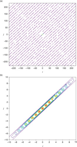
As the uniformly distributed coarse-resolution innovations are analysed in the first step with periodical extension, S is updated to S a according to eq. (2). As shown by the full-matrix structure of S a in a, S a is not diagonal (since M<N) but its non-zero off-diagonal elements are sparse and negligibly small. The diagonal elements of S a are also negligibly small outside the centre diagonal segment, as shown by the magnified structure of S a in b. Using eq. (2), the diagonal part of S a can be easily calculated from S and C. The analysis error power spectrum S a (k i ) given by the diagonal part of S a is plotted by the green×signsin , while the green curve, denoted by S a (k), plots the continuous counterpart of S a (k i ) obtained in the limit of Δk ≡ 2π/D→0 (or D→∞ with fixed Δx). As shown by the green×signs in comparison with the red+signs plotted for S(k i ) in , the error power spectrum is reduced by the first-step analysis dramatically for the first few wave numbers (from k i =0 to ∣k i ∣=2Δk), but the reduction decreases rapidly and becomes negligibly small as ∣k i ∣ increases to 6Δk and beyond. The analysis error correlation function C a(x) calculated from S a(k i ) by eq. (3) is plotted by the dashed green curve in . By comparing this green curve with the red curve in , the error correlation function is narrowed and thus the de-correlation length is reduced significantly when C b(x) is updated by C a(x). This is simply because the background errors are reduced mostly in long-wave structures as shown by the change of error power spectrum from S(k i ) to S a (k i ) in .
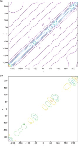
Fig. 4 (a) Full-matrix structure of S a. (b) Magnified structure of S a. The coloured contours plot the element value in m2s−2.
Note that <dd
T>=HBH
T+R, where <( )> denotes the expectation of ( ). Using this and eqs. (1) and (2), we obtain8
This implies that the power spectrum of the first-step analysis increment (as a spatially correlated random field) can be estimated by S(k i )−S a (k i ) in , which shows statistically that the first-step analysis increment contains mainly long-wave structure as a correction to the background field, while short-wave errors are left mostly unchanged. The correctable amounts of short-wave errors by the second-step analysis in the nested domain can be estimated statistically by the power spectrum of the second-step analysis increment in the form of S a1(k i ′)–S a2(k i ′), where k i ′=iΔk′ is the ith discrete wavenumber and Δk′ ≡ 2π/D′ (>Δk) is the minimum resolvable wavenumber associated with the nested domain of length D′, S a1(k i ′) is the power spectrum of the first-step analysis, that is, S a (k i ) projected in the wavenumber space of {k i ′}, and S a2(k i ′) is the power spectrum of the second-step analysis estimated similarly by using eq. (2) but in the space of {k i ′}, with S(k i ) replaced by S a1(k i ′). Note that S a1(k i ′) - S a2(k i ′)<S a1(k i ′) and S a1(k i ′) is bounded by S a (k i ), so the power spectrum of the second-step analysis increment is bounded below S a (k i ) and its detailed evaluation is omitted in this paper.
a shows the structure of the benchmark A that is precisely computed [either from A=F N H S a F N or from eq. (1b) by inverting HBH T+R in the space of the periodically extended coarse-resolution innovations within the extended domain of −D/2–3L≤x≤D/2+3L]. The structure of approximately calculated A by A ij =σ e 2 C a(x i –x j ) according to eq. (3) is largely the same as that shown for the benchmark A in a except that all the contour lines become exactly straight (not shown). b shows that the deviation of the approximately calculated A from the benchmark A is very small (within ±0.012 m2s−2) and the deviation reaches a local maximum of 0.0116 m2s−2 (or minimum of −0.0115 m2s−2) at the point marked by the +(or −) sign on the diagonal line. Note that the diagonal point marked by the +(or −) sign in b corresponds to a grid point that is collocated with a coarse-resolution innovation (or located in the middle between two adjacent coarse-resolution innovations). At such a grid point, the analysis error variance given by the diagonal element of the benchmark A is maximally (or minimally) reduced to 3.541 (or 3.565) m2s−2, while the diagonal elements of the approximately calculated A all have the same constant value of σ e 2=3.553 m2s−2, and this constant value accurately captures the true domain averaged analysis error variance (=3.553 m2s−2) given by the mean of the diagonal elements of the benchmark A. The correlation structure (not shown) intercepted from the benchmark A in a across the diagonal point marked by the+(or −) sign in b is almost the same as the approximately calculated analysis error correlation potted by the dotted blue curve in , and the difference is extremely small, confined between −0.0022 and 0.0028 (or −0.0006 and 0.0065).
Fig. 5 (a) Structure of benchmark A plotted by colour contours every 0.5 m2s−2. (b) Deviation of approximately calculated A from benchmark A plotted by solid (or dashed) contours at 0.01 (or −0.01) m2s−2. The deviation in (b) reaches the maximum (or minimum) of 0.01156 (−0.01145) m2s−2 at the point marked by the +(or −) sign on the diagonal, and this diagonal point corresponds to a grid point that is collocated with a coarse-resolution innovation (or located in the middle between two adjacent coarse-resolution innovations).
The single-step-analysed increment produced by SE with 20 iterations is denoted by Δa 20 and plotted by the dashed red curve in . This curve is not very close to the solid black curve plotted for the benchmark analysis increment, denoted by Δa, in . The error of Δa 20, evaluated by e 20=Δa 20−Δa, is shown by the dashed red curve in , and the domain averaged RMS value of e 20 is 0.883 ms−1 as listed in the first row of . The solid green curve in shows the analysis increment produced by the first step (of TEA, TEB, or TEC) with 20 iterations, and this first-step increment is denoted by Δa I-20. As Δa I-20 is produced by analysing only the 20 coarse-resolution innovations, the dashed green curve is not very close to the black benchmark curve, and its domain averaged RMS error with respect to the black benchmark curve in is 0.713 ms−1, as listed in the second row of . However, Δa I-20 is close to its own benchmark analysis increment, denoted by Δa I (not shown) and obtained directly from eq. (1a) for the coarse-resolution innovations only. The domain averaged RMS error of Δa I-20 with respect to Δa I is 0.321 ms−1 as listed in the third row of .
Fig. 6 Analysis error e 20 (or e 100) from SE with 20 (or 100) iterations plotted by dashed (or solid) red curve, analysis error e A20 (or e A100) from TEA with 20 (or 100) iterations plotted by dashed (or solid) blue curve, and analysis error e B20 (or e C20) from TEB (or TEC) with 20 iterations plotted by dot-dashed cyan (or grey) curve.
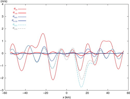
Table 1. Entire-domain averaged RMS errors (in ms−1) for the analysis increments obtained from SE, Step-I, TEA, TEB and TEC applied to the first set of innovations with periodic extension and consecutively increased n, where n is the number of iterations and Step-I stands for the first-step analysis (in TEA, TEB or TEC). All the RMS errors are evaluated with respect to the benchmark analysis increment Δa except for those in the third row where the RMS errors are evaluated versus Δa I – the benchmark for the first-step analysis itself, obtained directly from eq. (1a) for the coarse-resolution innovations only
The dashed blue, dotted cyan and dot-dashed grey curves in show the two-step-analysed increments denoted by Δ a A20, Δa B20 and Δa C20 and produced by TEA, TEB and TEC, respectively, with 20 iterations. The dashed blue curve from TEA is very close to the black benchmark curve, but the dotted cyan curve from TEB and dot-dashed grey curve from TEC are not close to the benchmark curve. Their errors, evaluated by e A20=Δa A20−Δa, e B20=Δa B20−Δa and e C20=Δa C20−Δa are plotted by the dashed blue, dot-dashed cyan and grey curves in , respectively. Their domain averaged RMS errors are 0.316, 0.806 and 0.661 ms−1, respectively, as listed in the last three rows of the first column in . As shown, with 20 iterations, the analysis from SE is much less accurate than that from TEA, slightly less accurate than that from TEB, and moderately less accurate than that from TEC.
When the iteration number, denoted by n, increases from 20 to 50, the analysis errors decrease by 3.1 times in SE, 3.8 times in TEA, 1.9 times in TEB and by 1.6 times in TEC, as shown in the second column of . In this case, the analysis from SE becomes more accurate than those from TEB and TEC but is still much less accurate than that from TEA. When n increases from 50 to 100, the analysis errors further decrease by 3.2 times in SE and by 4.9 times in TEA, but they no longer decrease in TEB and TEC, as shown in the third column of . In this case, the analysis error from TEA, denoted by e A100, is very small over the entire analysis domain, as shown by the solid blue curve in , while the analysis error from SE, denoted by e 100, is very small only inside the nested domain but not so outside the nested domain as shown by the solid red curve in . When n increases beyond 100, the iterative procedure in SE converges slowly and reaches the final convergence at n=309 with the RMS error finally reduced to 0.019 ms−1, while the iterative procedure in TEA converges quickly and reaches the final convergence at n=141 with the RMS error finally reduced to 0.007 ms−1 which is slightly smaller than the final RMS error from SE, as shown in the last column of .
3.3. Results for the second set of innovations with periodic extension
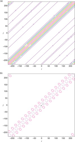
As the coarse-resolution innovations are non-uniformly distributed in the second set, the benchmark A can no longer be computed from A=F N H S a F N but still can be precisely computed from eq. (1b). The structure of this benchmark A is shown in a. As shown, the contour lines are still largely diagonal-parallel but contain irregular variations with M local minima corresponding to the M non-uniformly distributed coarse-resolution innovations. The approximately calculated A is the same as that for the uniformly distributed coarse-resolution innovations. The deviation of the approximately calculated A from the benchmark A in a is no longer very small as shown in b, and the deviation reaches the maximum of 0.639 m2s−2 (or minimum of −1.131 m2s−2) at the point marked by the +(or −) sign on the diagonal line in b. The approximately calculated σ e 2 (=3.553 m2s−2) is no longer equal to but still very close to the domain averaged analysis error variance (=3.634 m2s−2) given by the mean of the diagonal elements of the benchmark A in a. The correlation structure intercepted from the benchmark A in a across the diagonal point marked by the +(or −) sign in b is denoted by C a+(x) [or C a− (x)] and plotted by the dotted green (or purple) curve in . As shown, the dotted green (or purple) curve is slightly wider (or narrower) than the dotted blue curve for the approximately calculated analysis error correlation that is the same as that in . The difference between the dotted green (or purple) curve and the dotted blue curve is confined between −0.08 and 0.001 (or −0.001 and 0.04).
Fig. 7 As in but for the non-uniform coarse-resolution innovations in the second set. The contours in (a) are plotted every 1 m2s−2. The contours in (b) are plotted at ±0.2, ±0.5 and −1 m2s−2. The deviation in (b) reaches the maximum value of 0.639 m2s−2 (or minimum value of −1.131 m2s−2) at the diagonal point marked by the +(or −) sign.
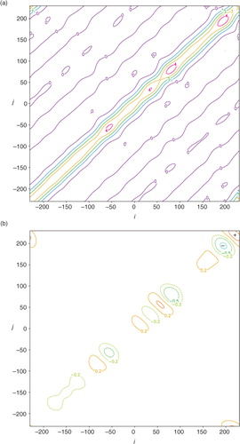
Fig. 8 As in but for the second set of innovations. The dotted green (or purple) curve plots C a+(x) [or C a− (x)] – the correlation structure intercepted from the benchmark A in a across the point marked by the +(or −) sign in b.
![Fig. 8 As in Fig. 2 but for the second set of innovations. The dotted green (or purple) curve plots C a+(x) [or C a− (x)] – the correlation structure intercepted from the benchmark A in Fig. 7a across the point marked by the +(or −) sign in Fig. 7b.](/cms/asset/cb33233f-6555-4031-9073-3f2c918fd8b0/zela_a_11830317_f0008_ob.jpg)
The above results show that the approximately calculated A is still good approximation of the benchmark A. Because of this, the results obtained from the second set of innovations are qualitatively the same as those obtained for the first set of innovations in the previous subsection. In particular, as shown in and and , with 20 iterations, the analysis increment Δa 20 from SE is still less accurate than both Δa B20 from TEB and Δa C20 from TEC, and is much less accurate than Δa A20 from TEA. When the iteration number n increases from 20 to 50 and then to 100, the analysis from SE gradually becomes more accurate than those from TEB and TEC but is still much less accurate than that from TEA. When n increases beyond 100, the iterative procedure reaches the final convergence at n=324 in SE with the RMS error finally reduced to 0.029 ms−1, and the iterative procedure reaches the final convergence at n=135 in TEA with the RMS error finally reduced to 0.039 ms−1, which is slightly larger than the final RMS error from SE, as shown in the last column of .
Fig. 9 As in but for the second set of innovations.
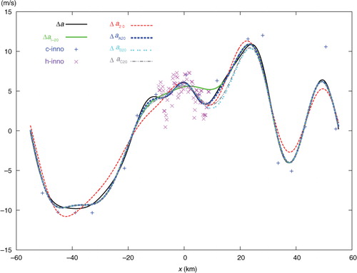
Fig. 10 As in but for the second set of innovations.
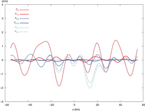
Table 2. As in but for the second set of innovations with periodic extension
3.4. Results for the second set of innovations without periodic extension
In the previous two subsections, the innovations and analysis increments are extended periodically with the analysis domain. The periodic extension is used to facilitate the derivation of the spectral formulation in eq. (2) for efficiently calculating σ e 2 C a(x) in eq. (3). But the calculated σ e 2 C a(x) can be modified and applied to the two-step analysis without periodic extension as explained below. As shown by the dotted blue curve in , C a(x) becomes almost zero as ∣x∣ increases to 3L (=30 km=3×41.67Δx) and beyond (but within the primary period defined by ∣x∣≤D/2). Thus, once σ e 2 C a(x) is approximately calculated from S a (k i ) as a periodic function according to eq. (3), it can be modified simply by setting C a(x) to zero for ∣x∣>D/2. This modified σ e 2 C a(x) can be used to update the background error covariance in the second step without periodic extension as long as D/2≥3L. [Note that, if D/2<3L, σ e 2 C a(x) can be calculated from S a (k i ) by imaginarily increasing N, say, to N′ with D′=N′Δx>6L in eq. (3), so the calculated σ e 2 C a(x) can be modified by letting C a(x) goes zero for ∣x∣>D′/2.]
With the above-modified σ e 2 C a(x), the two-step experiments (TEA, TEB and TEC) are performed in this subsection by using the second set of innovations without periodic extension. The SE and the benchmark analysis are also performed without periodic extension. In this case, the benchmark A is computed from eq. (1b) for the original M coarse-resolution innovations without periodic extension. As shown in a, this benchmark A has the same structure as that in a in most areas except for those around the four corners, and the differences around the four corners are caused by the removal of periodic extension.
Fig. 11 As in but without periodic extension. The contours in (b) are plotted at ±0.2, ±0.5, ±1, ±3, −5 and −7 m2s−2.
When A is calculated approximately by using the above modified σ e 2 C a(x), it has zero value for the elements at and around the two off-diagonal corners, and its deviation from the benchmark A in a is shown in b. As shown, the deviation is near zero at and around the two off-diagonal corners but becomes large at and near the two diagonal corners. The large deviations around the two diagonal corners, however, have little impact on the second-step analysis in TEA because their associated grid points are not only outside but also distant away from the nested domain beyond the effective correlation range (≈10 km, as shown by the dotted blue curve in ). With the two diagonal corner areas excluded, the deviation in b has essentially the same structure as that in b. This implies that the above approximately calculated A is still a good approximation of the benchmark A in a. Therefore, as shown in and , the results obtained without periodic extension are qualitatively the same as those obtained with periodic extension in the previous subsection.
Fig. 12 As in but without periodic extension.
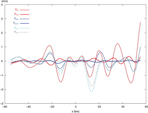
Table 3. As in but without periodic extension
4. Numerical experiments for two-dimensional cases
4.1. Description of data and experiments
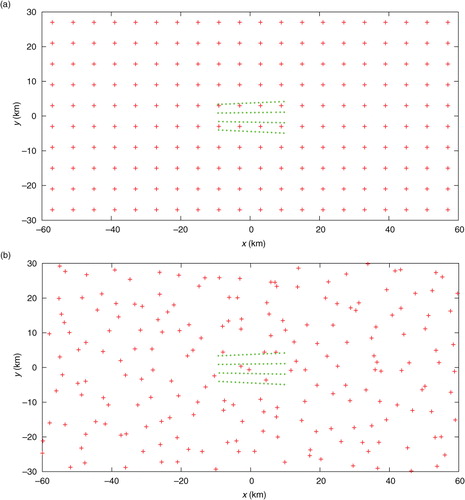
For the two-dimensional experiments performed in this section, the observational data and model-produced background field are taken from the same sources as those cited in Section 3.1 except for the following treatments. First, the two-dimensional analysis domain size is set to D x =N x Δx=120 km and D y =N y Δy=60 km, respectively, with N x =120, N y =60 and Δx=Δy=1 km. Second, innovations are generated in two sets. In the first (or second) set, the coarse-resolution innovations are generated by subtracting the background values from interpolated observations at M (= M x ×M y =20×10=200) points distributed uniformly (or non-uniformly) over the analysis domain as shown by the red+signs in a (or 13b), while the high-resolution observation innovations are generated by subtracting the background values from the original observations at M′ (=68) observational points, marked by the green dots in a (or 13b), in the nested domain of D x /6=20 km long and D y /6=10 km wide (see the rectangle plotted by the thin black lines in and or 20). The high-resolution innovations are spaced every 1.2 km in the radial direction along each radar beam, and the radar beams are spaced every 1.6° in the azimuthal direction.
Fig. 13 (a) Uniformly distributed coarse-resolution innovation points plotted by red+signs over the analysis domain, and high-resolution innovation points plotted by the green dots in the nested domain of D x /6=20 km long and D y /6=10 km wide. (b) As in (a) but for the second set in which the coarse-resolution innovations are not uniformly distributed. The coarse-resolution innovations in (a) are spaced every Δx co=6 km (or Δy co=6 km) in the x-direction (or y-direction). The domain-averaged resolution for the non-uniformly distributed coarse-resolution innovations in (b) is estimated also by Δx co ≈ 6 km (or Δy co ≈ 6 km) in the x-direction (or y-direction).
The background and observation error variances are set to σ b 2=52 m2s−2 and σ o 2=2.52 m2s−2, respectively, as in Section 3.1. The background error correlation function C b(x) is modelled by the same double-Gaussian form as in eq. (5) except that x 2 is replaced by ∣x∣2 and L=10Δx (=10 km). The periodic extension of C b(x) can be made in the x and y directions for each Gaussian function in the same way as shown in (17c) of CitationXu and Wei (2011). The periodically extended C b(x) is not exactly but nearly isotropic (not shown). By applying the DFT to the periodically extended σ b 2 C b(x, y), the background error power spectrum can be calculated in the discrete form of S(k i , k j ). For the double-Gaussian form of C b(x), S(k i , k j ) can be also derived analytically (not shown) as a two-dimensional extension of eq. (6) [see (17)–(18) of Xu and Wei, Citation2011]. Similar to the one-dimensional case discussed in Section 3.2, S(k i , k j ) approaches its continuous counterpart S(k)=S(k x , k y ) in the limit of Δk x ≡2π/D x →0 and Δk y ≡2π/D y →0, where k≡(k x , k y ) is the two-dimensional wavenumber. The diagonal matrix S can be constructed from S(k i , k j ) by converting the double indices (i, j) into a single index and then placing the N x N y elements of S(k i , k j ) along the diagonal of S.
The observation errors are assumed to be spatially uncorrelated, so R=σ o 2 I in the innovation space (without periodic extension). For each set of innovations, the benchmark analysis is again computed directly and precisely from eq. (1a), while the single-step analysis in SE is obtained, with a limited number of iterations, by minimising the same form of cost-function as in eq. (7) but formulated for the two-dimensional case. Three types of two-step experiments are designed and named similarly to those for the one-dimensional case in Section 3. They are (1) TEA in which the ijth element of B is updated to σ e 2 C a(x i − x j ) from eq. (4) in the second step, (2) TEB in which B is not updated and (3) TEB in which the ijth element of B is updated to σ e 2 C b(x i −x j ) in the second step.
4.2. Results for the first set of innovations without periodic extension
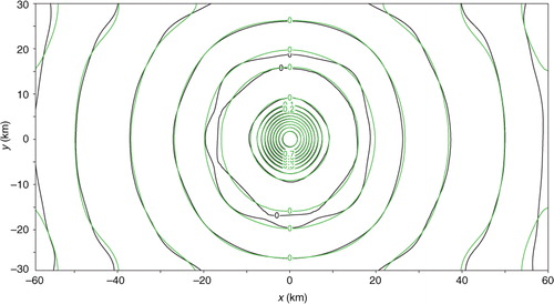
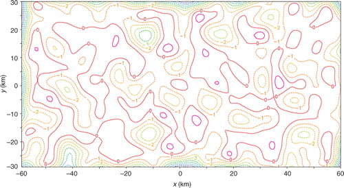
When the uniformly distributed coarse-resolution innovations from the first set are analysed in the first step without periodical extension, S can be updated to S a approximately according to the two-dimensional spectral form of eq. (2), as explained in Section 2.3. Again, because M<N, S a is not diagonal, but its non-zero off-diagonal elements are sparse and negligibly small, and this feature (not shown) is similar to the one-dimensional case in a. Thus, the diagonal part of S a gives the analysis error power spectrum S a (k i , k j ) approximately. The analysis error covariance function σ e 2 C a(x) can be calculated from S a (k i , k j ) according to eq. (4) and then modified by setting C a(x) to zero for ∣x∣>D x /2 or ∣y∣>D y /2 (for the same reason as explained in Section 3.4). The calculated C a(x−x c) is shown by the green contours for x c=(0, 0) in , where x c denotes the correlation centre and the analysis domain is centred at x=(0, 0). The benchmark A is computed from eq. (1b) by inverting HBH T+R without periodic extension. The benchmark correlation pattern is plotted by the black contours also for x c=(0, 0) in , and this correlation pattern corresponds to the central column (or row) of the benchmark A normalised by its diagonal element. As shown, the approximately calculated C a(x) matches the benchmark correlation closely for all the non-zero contours. Similar close matches are seen when x c is moved away from the domain centre but still within the interior domain with its distance from the domain boundaries larger than the effective correlation range (≈10 km) defined by the radius of the first zero-contour circle of C a(x) in .
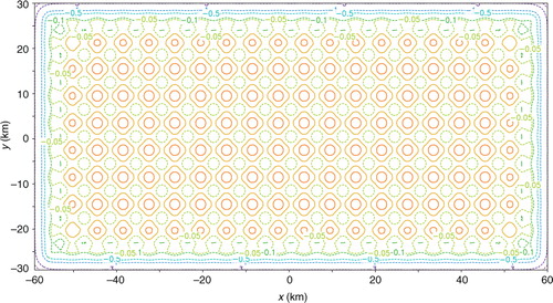
Fig. 14 C a(x−x c) plotted by the green contours for x c=(0, 0), and benchmark correlation pattern plotted by the black contours with x c also placed at x=(0, 0) – the centre of the analysis domain. Here, x c denotes the correlation centre.
The N (=N x N y ) diagonal elements of the benchmark A give the analysis error variances at the N x xN y grid points over the analysis domain. The approximately calculated analysis error variance is σ e 2=3.153 m2s−2, and its deviation from the benchmark analysis error variance is plotted by coloured contours in . As shown, the deviation is very small and confined between ±0.075 m2s−2 over the interior domain that covers the nested domain. The benchmark analysis error variances have an averaged value of 3.150 m2s−2 over the interior domain, and this averaged value is closely matched by σ e 2 (=3.153 m2s−2). Towards the domain boundaries within the effective correlation range (≈10 km), the deviation drops rapidly below −0.1 m2s−2 as shown in , and this rapid drop corresponds to the rapid increase in the benchmark analysis error variance caused by the absence of coarse-resolution innovation outside the analysis domain. The large negative deviations around the domain boundaries, however, have little impact on the second-step analysis in TEA because their associated grid points are not only outside but also distant away from the nested domain beyond the above defined effective correlation range. Thus, the above approximately calculated A is a good approximation of the benchmark A for the second-step analysis.
Fig. 15 Deviation of σ e 2 (= 3.1527 m2s−2) from benchmark analysis error variance plotted by contours at 0, ±0.05, −0.1, −0.2, −0.5, −1, −3 and −5 m2s−2 over the analysis domain.
The analysis increment from SE applied to the first set of innovations with 20 iterations is denoted by Δa 20 and plotted by the red contours in in comparison with the black contours for the benchmark analysis increment, denoted by Δa. As shown, the red contours of Δa 20 match the benchmark black contours not as closely as the blue contours of Δa A20 – the analysis increment from TEA, especially in the nested domain. The error of Δa 20, evaluated by e 20=Δa 20−Δa, is shown by the red contours in in comparison with the blue contours for the error of Δa A20, evaluated by e A20=Δa A20−Δa. As shown, e 20 is both positively and negatively larger than e A20 in the nested domain, where the positive (or negative) maximum of e 20 is 2.90 (or −1.66) ms−1 while the positive (or negative) maximum of e A20 is 0.84 (or −0.84) ms−1. The nested-domain averaged RMS error is 1.11 ms−1 in SE but is only 0.32 ms−1 in TEA. The entire-domain averaged RMS error from SE is significantly larger than that from TEA, slightly large than that from TEC, but smaller than that from TEB, as shown in the first column of .
Fig. 16 Benchmark analysis increment Δa plotted by black contours, analysis increment Δa 20 from SE with 20 iterations plotted by red contours, and analysis increment Δa A20 from TEA with 20 iterations plotted by blue contours. The rectangle plotted by thin black lines shows the nested domain.
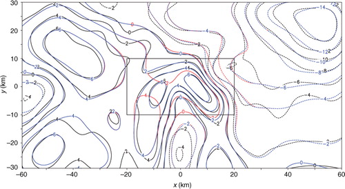
Fig. 17 Analysis error e 20 from SE and analysis error e A20 from TEA with 20 iterations plotted by red and blue contours, respectively. The rectangle plotted by thin black lines shows the nested domain.
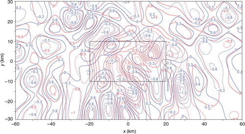
Table 4. As in but for the first set of innovations in the two-dimensional case as shown in a
When the iteration number n increases from 20 to 50, the analysis from SE becomes more accurate than that from TEC but is still less accurate than that from TEA as shown in the second column of . When n increases from 50 to 100, the analysis from SE is also still less accurate than that from TEA, as shown in the third column of . The iterative procedure in TEA reaches the final convergence at n=81 with the RMS error finally reduced to 0.059 ms−1, while the iterative procedure in SE reaches the final convergence at n=312 with the RMS error finally reduced to 0.043 ms−1, which is smaller than the final RMS error from TEA, as shown in the last column of .
4.3. Results for the second set of innovations without periodic extension
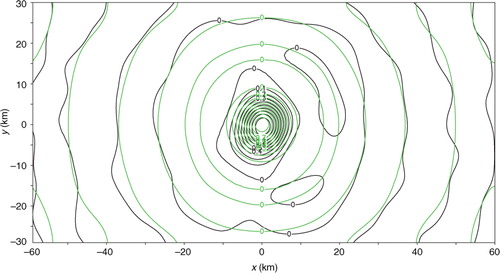
When the non-uniformly distributed coarse-resolution innovations from the second set are analysed in the first step without periodical extension, the analysis error covariance function σ e 2 C a(x) can still be calculated approximately from S a (k i , k j ) according to eq. (4) and then modified in the same way as in the previous subsection, and A ij =σ e 2 C a(x i −x j ) gives the ijth element of A approximately. The calculated C a(x−x c) is re-plotted by the green contours for x c=(0, 0) in , which is the same as that in . However, the benchmark A computed from eq. (1b) with the non-uniformly distributed coarse-resolution innovations becomes different from that in the previous subsection, and so do the benchmark analysis error variances (given by the diagonal elements of the benchmark A at the N x ×N y grid points). The benchmark correlation pattern is shown by the black contours for x c=(0, 0) in , which corresponds to the central column (or row) of the benchmark A normalised by its diagonal element. As shown, the approximately calculated C a(x) still loosely matches the benchmark correlation for all the non-zero contours. Similar matches are seen for x c≠(0, 0) but still within the interior domain.
Fig. 18 As in but for the second set of innovations.
The calculated analysis error variance is still σ e 2=3.153 m2s−2 as in the previous subsection, and its deviation from the benchmark analysis error variance is shown by the colour contours in . As shown, the deviation is no longer small but is mostly between −2 and 1 m2s−2 within and around the nested domain. The benchmark analysis error variances have an averaged value of 3.77 m2s−2 over the nested domain, and this averaged value is much better matched by σ e 2 (=3.153 m2s−2) than the background error variance σ b 2 (=25 m2s−2). Large deviations are seen near the domain boundaries in , but they have little impact on the second-step analysis in TEA for the same reason as explained in the previous subsection. Thus, the above estimated A is still a reasonably good approximation of the benchmark A for the second-step analysis.
Fig. 19 As in but for the second set of innovations with contours plotted every 1 m2s−2.
The analysis increment from SE (or TEA) applied to the second set of innovations with 20 iterations is denoted again by Δa 20 (or Δa A20) and the benchmark analysis increment is denoted by Δa. The error of Δa 20, evaluated by e 20=Δa 20−Δa, is plotted by the red contours in in comparison with the blue contours for e A20=Δa A20−Δa. As shown, e 20 is both positively and negatively larger than e A20 in the nested domain, where the positive (or negative) maximum of e 20 is 2.59 (or −2.02) ms−1 but the positive (or negative) maximum of e A20 is 0.76 (or −1.08) ms−1. The nested-domain averaged RMS error is 1.05 ms−1 in SE but is only 0.39 ms−1 in TEA. The entire-domain averaged RMS errors are listed in the first column of , and they are similar to those in the first column of .
Fig. 20 As in for the second set of innovations.
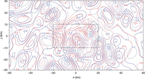
Table 5. As in but for the second set of innovations as shown in b
When the iteration number n increases from 20 to 50 and then to 100, the results are similar to those obtained in the previous subsection as shown in the second and third columns of in comparison with those in . As shown in the last column of , the iterative procedure in TEA converges at n=59 with the RMS error finally reduced to 0.111 ms−1, while the iterative procedure in SE converges at n=237 with the RMS error finally reduced to 0.064 ms−1. These results are also similar to those listed in the last column of .
4.4. Results and discussion on computational efficiency
As explained at the end of Section 3.2, the second step in the two-step analysis is performed in a nested domain with a much reduced control vector dimension. As a result, the second-step analysis takes much less computational time (measured by CPU – Computer's central processing unit) than the first-step analysis. In particular, with n=20 for the two-dimensional case presented in this subsection, the second-step analysis takes merely 0.16 s of CPU time while the first-step analysis takes 105.90 s. The CPU time for the single-step analysis in SE is 108.20 s. In the two-step analysis, the analysis error covariance function is calculated approximately and very efficiently, and therefore, its required CPU time is relatively small (merely 6.32 s for the two-dimensional cases presented in this section). For real-time applications, the analysis error covariance function can always be pre-calculated and thus will not cost any CPU time in real-time run. Thus, with the same number of iterations, the two-step analysis costs no more CPU time than the single-step analysis. Moreover, as shown in , the two-step analysis converges much faster than the single-step analysis. Therefore, to reach the same accuracy, the computational cost for the two-step analysis should be much smaller than that for the single-step analysis.
Furthermore, since the first step in the two-step analysis analyses only the coarse-resolution observations, the grid resolution can be properly coarsened in the first step with no loss of information content from the coarse-resolution observations and thus no loss of analysis accuracy (see Section 4 of Xu, Citation2011), while the original high-resolution grid (used by the single-step analysis to cover the entire domain) is reduced to cover only the nested domain for the control vector c II in the second step of the two-step analysis (as explained at the end of Section 3.1). For example, when the grid resolution is coarsened to Δx=Δy=2 km in the first step for the two-dimensional case in this subsection, the RMS error (= 0.407 ms−1) of the first-step analysis with n =20 is very close to the value of 0.406 ms−1 listed for Δx=Δy=1 km in the third row of , but the required CPU time is reduced sharply from 105.90 to 7.18 s. In this particular case, the two-step analysis with n=20 costs only 8.34 s of CPU time which is much smaller than the CPU time (108.20 s) required by the single-step analysis with the same n =20. Such a two-grid approach can make the two-step analysis not only much more efficient but also substantially more accurate than the single-step analysis with the same limited number of iterations.
5. Summary and conclusion
In this study, a two-step variational method is designed to analyse broadly distributed coarse-resolution observations and locally distributed high-resolution observations in two separate steps. As the analysed field obtained with coarse-resolution observations in the first step is used as the updated background field for assimilating high-resolution observations in the second step, the background error covariance should be also updated in the second step by the analysis error covariance from the first step. Due to the fact that the analysis error covariance matrix is too large to directly and precisely compute [see eq. (1b)] in operational data assimilation, how to objectively estimate or efficiently compute the analysis error covariance in the first step for updating the background error covariance in the second (or any subsequent) step becomes the first challenging issue encountered in the two-step (or any multistep) variational method. This issue is very important for multiscale and multistep variational analyses but has been largely ignored or avoided by previous studies as reviewed in the introduction. To attack this issue, a new approach is proposed in which spectral formulations are derived and simplified to approximately and very efficiently calculate the analysis error covariance functions [see eqs. (2–4) and the Appendix]. Verified against their respective benchmark truths, the calculated analysis error covariance functions are shown to be very good approximations for uniformly distributed coarse-resolution observations (see for a one-dimensional case and and for a two-dimensional case) and fairly good approximations for non-uniformly distributed coarse-resolution observations (see and for one-dimensional cases and and for a two-dimensional case), at least, over the nested domain and surrounding areas within the analysis domain.
Having the above first issue addressed, the next important question is whether and under what conditions the above calculated analysis error covariance function can make the two-step analysis more accurate than the conventional single-step analysis. To answer this question, numerical experiments are performed for idealised one- and two-dimensional cases to compare the two-step analyses with their respective counterpart single-step analyses with various limited numbers of iterations (to mimic the computationally constrained situations in operational data assimilation). In each set of these experiments, the background error covariance is assumed exactly known and accurately modelled for the single-step analysis, so the optimal analysis can be precisely computed and used as a benchmark to evaluate the accuracy of the single-step analysis versus its counterpart two-step analysis. The major findings are summarised below:
By using the approximately calculated analysis error covariance function to update the background error covariance in the second step, the two-step analysis (performed in the two-step experiment named TEA) can be significantly more accurate than the single-step analysis (performed in the control experiment named SE) as long as the iteration number is not sufficiently large. Only when the iteration number becomes so large that the single-step analysis reaches the final convergence or nearly so, the single-step analysis can become slightly more accurate than the two-step analysis (as shown by the results from TEA versus those from SE in Tables (Citation1–Citation5)).
If the background error covariance is not updated (or only the background error variance is updated) in the second step, then the two-step analysis can be as accurate as (or slightly more accurate than) the single-step analysis only if the iteration number is severely limited to a fraction of the total number of iterations needed for the final convergence of the single-step analysis [as shown by the results from TEB (or TEC) versus those from SE in Tables (Citation1–Citation5)].
The two-step analysis (in TEA) converges much faster and thus costs much less computational time than the single-step analysis to reach the same accuracy. Furthermore, since the first step in the two-step analysis analyses only the coarse-resolution observations, the grid resolution can be properly coarsened in the first step with the original high-resolution grid used only over the nested domain in the second step. With this two-grid approach, the two-step analysis (in TEA) can be not only more accurate but also much more efficient than the single-step analysis with the same limited number of iterations.
In our idealised experiments, the coarse-resolution observations are sparsely taken from the same source as the high-resolution observations, so their error variance is the same as that (σ o 2≈2.52 m2s−2) for the high-resolution observations but much smaller than that (σ o 2≈42 m2s−2) estimated for operational radiosonde wind observations (see of Xu and Wei, Citation2001). To accurately represent the latter case, computer-generated uncorrelated Gaussian random numbers are used to simulate coarse-resolution (or high-resolution) observation errors with σ o=4 ms−1 (or σ o=2.5 ms−1) and produce their associated coarse-resolution (or high-resolution) innovations by subtracting computer-generated spatially-correlated Gaussian random background errors [with σ b=5 ms−1 and C b(x) modelled by eq. (5)]. Additional experiments are performed with these simulated innovations and the results (not shown) are qualitatively the same as those presented in this paper. Thus, the major findings summarised above are sufficiently robust (for different settings of observation error variance and background error covariance and for different samplings of various innovations).
The two-step analysis is proposed in this paper primarily for variational data assimilation with coarse-resolution observations broadly distributed over the entire model domain and high-resolution observations locally distributed in a nested domain, but it can be also extended and applied to situations in which both coarse and high-resolution observations are present throughout the entire model domain and analysed separately in two steps. In this case, the two-step analysis still can be more accurate and computationally more efficient than the single-step analysis as long as the iteration number is not sufficiently large for the single-step analysis and the iteration number is properly further reduced for the two-step analysis (to gain extra computational efficiency, especially if the first step is performed on a properly coarsened grid as explained earlier). For such an extended application, according to our additional experiments (not presented in this paper), the performance gain of the two-step analysis over the single-step analysis is reduced but still significant.
As mentioned in the introduction, double Gaussians have been used to model the background error correlation in variational data assimilation at NCEP with each Gaussian computed separately by the recursive filter (Wu et al., Citation2002; Purser et al., Citation2003). When such a recursive filter is used in a two-step variational analysis, using a single Gaussian to model the background error correlation in each step can reduce the computational cost. The true background error correlation, however, may not be adequately modelled by a single Gaussian. In this case, the spectral formulation derived in this paper should be modified to consider the inaccuracy of the background error correlation modelled by the single-Gaussian. Such a modification is under our investigation.
The two-dimensional spectral formulations derived in this paper can be extended and used to efficiently calculate the error covariance functions in the three-dimensional space for univariate analyses of sparsely spaced vertical profiles of observations, such as operational radiosondes or vertical profiles of horizontal winds produced by the velocity-azimuth display method from radar radial-velocity measurements. For those data, we may assume that the error correlation structure in the vertical direction is not much affected by the analysis, so we only need to update the error variance and horizontal correlation structure on each and every vertical level essentially in the same way as shown for the two-dimensional cases in Section 4. Such an extension will be explored with the real-time variational data assimilation system of CitationGao et al. (2013), in which the analyses are all univariate and performed in two steps. The two-dimensional spectral formulations can be also extended for multivariate analyses and applied to the multistep radar wind analysis system of CitationXu et al. (2015). Such an extension is currently being developed and the results will be presented in a follow-up paper.
6. Acknowledgements
The authors are thankful to Prof. S. Lakshmivarahan of the University of Oklahoma (OU) and the three anonymous reviewers for their comments and suggestions that improved the presentation of the paper. The research work was supported by the ONR Grant N000141410281 and NSF grant AGS-1341878 to OU. Funding was also provided to CIMMS by NOAA/Office of Oceanic and Atmospheric Research under NOAA-OU Cooperative Agreement #NA11OAR4320072, U.S. Department of Commerce.
Related Research Data
References
- Derber J. , Bouttier F . A reformulation of the background error covariance in the ECMWF global data assimilation system. Tellus A. 1999; 51: 195–221.
- Derber J. , Rosati A . A global oceanic data assimilation system. J. Phys. Oceanogr. 1989; 19: 1333–1347.
- Gao J. , Smith T. M. , Stensrud D. J. , Fu C. , Calhoun K. , co-authors . A realtime weather-adaptive 3DVAR analysis system for severe weather detections and warnings. Weather Forecast. 2013; 28: 727–745.
- Hollingsworth A. , Lonnberg P . The statistical structure of short-range forecast errors as determined from radiosonde data. Part I: the wind field. Tellus A. 1986; 38: 111–136.
- Jazwinski A. H . Stochastic Processes and Filtering Theory. 1970; San Diego, CA: Academic Press. 376 pp.
- Li Z. , McWilliams J. C. , Ide K. , Farrara J. D . A multiscale variational data assimilation scheme: formulation and illustration. Mon. Weather Rev. 2015; 143: 3804–3822.
- Liu S. , Xue M. , Gao J. , Parrish D . Analysis and impact of super-obbed Doppler radial velocity in the NCEP grid-point statistical interpolation (GSI) analysis system. Extended abstract. 17th Conference on Numerical Weather Prediction. 2005; DC: Washington. Amer. Meteor. Soc., 13A-4.
- Lonnberg P. , Hollingsworth A . The statistical structure of short-range forecast errors as determined from radiosonde data. Part II: the covariance of height and wind errors. Tellus A. 1986; 38: 137–161.
- Parrish D. F. , Derber J. C . The national meteorological center's spectral statistical-interpolation analysis system. Mon. Weather Rev. 1992; 120: 1747–1763.
- Purser R. J. , Wu W.-S. , Parrish D. F. , Roberts N. M . Numerical aspects of the application of recursive filters to variational statistical analysis. Part II: spatially inhomogeneous and anisotropic general covariances. Mon. Weather. Rev. 2003; 131: 1536–1548.
- Wu W.-S. , Purser R. J. , Parrish D. F . Three-dimensional variational analysis with spatially inhomogeneous covariances. Mon. Weather Rev. 2002; 130: 2905–2916.
- Xie Y. , Koch S. , McGinley J. , Albers S. , Bieringer P. E. , co-authors . A space–time multiscale analysis system: a sequential variational analysis approach. Mon. Weather Rev. 2011; 139: 1224–1240.
- Xu Q . Measuring information content from observations for data assimilation: relative entropy versus Shannon entropy difference. Tellus A. 2007; 59: 198–209.
- Xu Q . Measuring information content from observations for data assimilation: spectral formulations and their implications to observational data compression. Tellus A. 2011; 63: 793–804.
- Xu Q. , Wei L . Estimation of three-dimensional error covariances. Part II: analysis of wind innovation vectors. Mon. Weather Rev. 2001; 129: 2939–2954.
- Xu Q. , Wei L . Estimation of three-dimensional error covariances. Part III: height-wind error correlation and related geostrophy. Mon. Weather. Rev. 2002; 130: 1052–1062.
- Xu Q. , Wei L . Measuring information content from observations for data assimilation: utilities of spectral formulations for radar data compression. Tellus A. 2011; 63: 1014–1027.
- Xu Q. , Wei L. , Nai K. , Liu S. , Rabin R. M. , co-authors . A radar wind analysis system for nowcast applications. Adv. Meteorol. 2015; 2015: 264515, 13.
- Xu Q. , Wei L. , Van Tuyl A. , Barker E. H . Estimation of three-dimensional error covariances. Part I: analysis of height innovation vectors. Mon. Weather. Rev. 2001; 129: 2126–2135.
7. Appendix
Algorithms for calculating the diagonal part of S a
1. One-dimensional case
For M<N in the one-dimensional case, as shown in (25) of CitationXu (2011), the ith diagonal element of Π=P
MN
SP
MN
T is given byA1
where N −≡Int[(1−N)/2], N +≡Int[N/2], M −≡Int[(1−M)/2]), M +≡Int[M/2], L −≡Int[(N −−M +)/M], L +≡Int[(N +−M −)/M], and S i+lM denotes the (i+lM)th diagonal element of S. Using eq. (A1), Π can be easily calculated from S by the following algorithm:
Do n=N −, … N +
if n≤0 then
l=Int[(n−M +)/M]
otherwise
l=Int[(n−M −)/M]
endif
i=n−lM
Π i =Π i +S n
enddo
In the above algorithm, Int[ ] denotes the integer part of [ ]. After this, the diagonal part of S a, with its ith diagonal element denoted by (S a) i , can be easily calculated by the following algorithm:
Do i=N −, … N +
if i≤0 then
l=Int[(i−M +)/M]
otherwise
l=Int[(i−M −)/M]
endif
n=i−lM
(S a) i =S i −S i 2/(Π n +νσ o 2)
enddo
In the above algorithm, C n =σ o 2 is used for R=σ o 2 I M and thus C ≡ F M RF M H=σ o 2 I M .
2. Two-dimensional case
As explained in Section 2.3, the diagonal part of S
a gives the analysis error power spectrum in the discrete form of (S
a
)
ij
=S
a
(k
i
, k
j
) in the two-dimensional wavenumber space, and so do the diagonal matrices S and Π. For M
x
<N
x
and M
y
<N
y
in the two-dimensional case, as shown in (32) of CitationXu (2011), the ijth diagonal element of Π=P
MN
SP
MN
T is given byA2
where N x−, N x+, M x−, M x+, L x− and L x+ (or N y , N y+, M y−, M y+, L y− and L y+) are defined for the x (or y) dimension in the same way as for their respective one-dimensional counterparts in eq. (A1), and S(i+lM x , j+l′M y ) denotes the [(i+lM x )(j+l′M y )]th diagonal element of S. Using eq. (A2), Π can be easily calculated from S by the following algorithm:
Do n=N x−, … N x+
if n≤0 then
l=Int[(n−M x+)/M x ]
otherwise
l=Int[(n−M x−)/M x ]
endif
i=n−lM x
Do n′=N y−, … N y+
if n′≤0 then
l′=Int[(n′−M y+)/M y ]
otherwise
l′=Int[(n′−M y−)/M y ]
endif
j=n′−l′M y
Πij=Πij+Snn′
enddo
enddo
After this, the diagonal part of S a, with its ijth diagonal element denoted by (S a) ij , can be easily calculated by the following algorithm:
Do i=N x−, … N x+
if i≤0 then
l=Int[(i−M x+)/M x ]
otherwise
l=Int[(i−M x−)/M x ]
endif
n=i−lM x
Do j=N y−, … N y+
if j≤0 then
l′=Int[(j−M y+)/M y ]
otherwise
l′=Int[(j−M y−)/M y ]
endif
n′=j−l′M y
(S a) ij =S ij −S ij 2/(Π nn’+ν x ν y σ o 2)
enddo
enddo