Impact of lake surface temperatures simulated by the FLake scheme in the CNRM-CM5 climate model

Abstract

The impact of lakes on climate is investigated in a set of global simulations performed with the CNRM-CM5 climate model coupled to the FLake lake scheme. First, offline simulations driven by ERA-Interim (ERA-I hereafter) reanalysis are performed on a limited set of lakes to find the best FLake parameters setting. Optimal values of lake depth, ice albedo and light extinction coefficient are defined by evaluating the model's performance in different climates for surface temperature and lake ice duration. Second, global simulations are performed with and without FLake to assess the impact of lake representation on the surface energy balance and the boundary layer characteristics. Results indicate that FLake simulates the lake surface temperature satisfactorily in an offline mode and that the use of FLake coupled to CNRM-CM5 improves some of the global biases found in the climate model. It is also shown that lakes impact the surface energy budget significantly at a regional scale; however, the impact on climate is rather limited. Finally, future developments related to the implementation of a more physical snow model and a water balance in FLake are discussed.

• climate modelling
• surface modelling
• lakes

1. Introduction

Lakes and inland water bodies represent approximately 3.5 % of the Earth's non-glaciated land surface areas (Verpoorter et al., 2014). These are characterised by high spatial variability and amplitude varying from a few hectares to several tens of thousands of square kilometres. Although lakes exhibit a clear surface temperature diurnal cycle, it remains lower than over continents due to a stronger heat capacity. Lake density is high in some regions, such as the Great Lake regions in North America and also in boreal regions (Downing et al., 2006; Verpoorter et al., 2014). Such regions are characterised by frost in early winter and by thawing in spring, which substantially alter the nature of the energy exchange between the surface and the atmosphere. The frost formation on a lake alters its radiative properties, such as albedo and emissivity, and has a direct impact on the surface temperature. Changes in surface properties modify the surface energy balance and the energy exchanges between the surface and the atmosphere. Moreover, snow accumulation on a frozen lake modifies its thermodynamic properties due to the insulating effect of snow, leading to a decoupling between the lake and the atmosphere. Inversely, during the spring break-up, the surface atmosphere exchanges will restart abruptly and impact the surface energy balance, which is one of the major components of the main climatic balances. The seasonal behaviour of lakes reinforces the notion that lakes can significantly influence the regional climate at various spatial scales. Bonan (1995) demonstrated that lakes were responsible for a cooling effect in summer, with a decrease in sensible heat flux, associated with an increase in the latent heat flux and, consequently, evaporation. Lofgren (1997) showed that summer evaporation and precipitation were reduced in the Great Lakes region, due to an enhancement of the stability in the atmospheric boundary layer. Dutra et al. (2010) showed the changes in the partition of energy fluxes in high latitudes and equatorial regions when accounting for lakes in global simulations driven by an atmospheric reanalysis.

In Numerical Weather Prediction (NWP) and climate models, substantial efforts have been dedicated to the modelling of natural and ocean surfaces at the expense of lake and urban areas. The increase in the horizontal resolution of NWP and climate models with improved computer power has enabled lakes of smaller extent to be distinguished. For this reason, accounting for lakes in such modelling systems has become challenging, especially in regions where lake fraction is high. Balsamo et al. (2012) shown that simulating subgrid lakes in global forecasts allowed reducing forecast errors at high latitudes especially during spring and summer, mainly because of the high thermal inertia of lakes. The FLake scheme (Mironov, 2008) was introduced (Salgado and Le Moigne, 2010) in the SURFEX (EXternalised SURFace) surface modelling platform (Le Moigne et al., 2012; Masson et al., 2013), which gathers the developments related to surface parameterisations performed over the last 20 yr at the Centre National de Recherches Météorologiques (CNRM). SURFEX uses a standardised interface (Best et al., 2004) for the coupling between the atmosphere and the surface. During a model run, each surface grid cell is constrained by air temperature, specific humidity, horizontal wind speed, pressure, solid and liquid precipitation rates, and long-wave and short-wave radiation. SURFEX uses a tiling approach where each grid cell is made up of four surfaces: one for nature, one for urban areas, one for seas and oceans, and one for lakes. The fraction of each tile is computed with the global ECOCLIMAP database (Masson et al., 2003; Faroux et al., 2013), which combines land cover maps and satellite information. Grid-cell averaged fluxes for momentum, sensible and latent heat and possibly chemical species and dust fluxes are computed, along with averaged surface temperature, direct and diffuse albedo and emissivity, and returned to the atmosphere. These quantities are used as lower boundary conditions for the atmospheric turbulence and radiation schemes. Finally, SURFEX presents the advantage that it can be used in offline mode (driven by realistic atmospheric fluxes) or fully coupled to any atmospheric model (inline mode) by providing a standard interface between the atmosphere and the surface. The offline mode is particularly well suited for evaluating all SURFEX parameterisations at the global scale using realistic atmospheric fluxes to avoid the systematic biases commonly found in the atmospheric models.

In 2011, the THAUMEX field campaign (Le Moigne et al., 2013) was carried out in southern France, where the FLake scheme was first validated offline against in situ lake water temperature profile and surface energy fluxes data collected on a Mediterranean Lagoon. Second, the first inline simulation with FLake coupled to the Meso-NH mesoscale model (Lafore et al., 1998) was performed in order to characterise the atmospheric boundary layer over the lagoon during a sea-breeze event. This recent study has improved confidence in the model's ability to represent lake–atmosphere exchanges consistently, underlying the importance of evaluating the FLake scheme at the global scale and analysing the behaviour of the lake–atmosphere coupling using a climate model. Nevertheless, the study of the water column heat budget during THAUMEX has demonstrated the value of simulating a surface skin temperature. FLake was not designed to simulate a skin temperature at the lake surface. Such a surface skin temperature is typically a few tenths of a degree lower than the water temperature below, but some studies indicate that the difference may be larger (Garrett et al., 2001), particularly in warm lakes. For this reason, a skin temperature parameterisation was developed in this study using the FLake scheme in order to improve the computation of the lake surface temperature.

To evaluate this new version of FLake at the global scale, some global offline simulations are performed, driven by ERA-I reanalysis (Simmons et al., 2007; Dee et al., 2011) over a 32-yr period (1979–2010). Second, fully coupled simulations are performed over the same time period using the global climate model of the CNRM, named CNRM-CM5. This climate model was adapted to be coupled to an updated SURFEX release, allowing the use of the FLake scheme. The complementarity of the offline and coupled approaches helps to fulfil the following objectives:

• Set the best configuration of FLake parameters, such as lake fraction, depth and extinction coefficient of light, albedo of water, ice and snow;

• Evaluate the FLake scheme offline at a global scale on the largest lakes. Simulations are compared to ARC-Lake products to assess the model's ability to retrieve the surface temperature and the number of frozen days of each lake;

• Run the model inline using the CNRM-CM5 climate model and evaluate the impact of the implementation of lakes in climate simulations, with the objective of using FLake in the next version of the CNRM-CM5 model developed within the framework of the CMIP6 intercomparison project.

2. FLake scheme

2.1. Model overview

FLake (Mironov, 2008) is a bulk-type numerical scheme developed to represent the thermodynamics of a lake. In particular, it computes the temporal evolution of the vertical lake temperature profile from the surface to the bottom, with the lake eventually becoming covered in ice and snow.

The unfrozen water temperature profile is represented by a mixed layer with a uniform temperature above a thermocline, the structure of which is parameterised using the concept of self-similarity (Kitaigorodskii and Miropolski, 1970). The same concept is used to describe the temperature structure of the ice and snow cover. An entrainment equation is used to calculate the mixed layer depth, based on the surface stress induced by wind and the thermally driven mixing. The model requires external parameters, the most relevant of which are the lake depth and the attenuation coefficient of light into the water. This coefficient controls the penetration of solar radiations within the water body. Lake depth is provided by the Global Lake Depth database (Kourzeneva, 2010), whereas no spatialised information is available for the extinction coefficient, which is set up uniformly over the globe.

One recent change was the introduction of skin temperature in FLake. The objective is to simulate a surface temperature representative of the energy budget at the lake surface, where the total derivative of temperature is in balance with the diffusion of the temperature plus a heat source, due to the divergence of the net radiation flux at the surface. Details of the computation of the skin temperature are provided in Appendix A.1. The thickness of the skin layer is assumed to be constant and equal to 1 mm. During a model time step, this new surface temperature is then used to compute the new surface heat fluxes in the atmosphere, the new thickness of the mixed layer and the new thermocline profile.

To evaluate FLake snow cover, simulations were made over land with the detailed snow model CROCUS (Vionnet et al., 2012) for points located at the same place as the 200 lakes (see Section 3.1). This complex snowpack model was developed primarily in support of avalanche forecasting, and more generally for all applications (including process studies), requiring a detailed representation of the vertical profile of the physical properties of snow. In addition to simulating macroscopic snowpack physical properties, they explicitly account for the time evolution of the snow microstructure driven by snow metamorphism, and the multiple feedback loops involving internal snow processes and the energy and mass balance at the air/snow and snow/ground interface (Brun et al., 1989, 1992; Jordan, 1991; Bartlett and Lehning, 2002).

2.2. Important model parameters

The spatial distribution of the lake at the global scale is given by the ECOCLIMAP database at 1-km resolution where the lake depth is given by Kourzeneva (2010). Some improvements have been made to separate lakes, wetlands and rivers in ECOCLIMAP using information from the 1-km Global Lakes and Wetlands Dataset (GLWD, Lehner and Döll, 2004), which distinguishes lakes, reservoirs, rivers and different kinds of wetlands. The use of GLWD has allowed the introduction, as lakes, of some large reservoirs that were missing in ECOCLIMAP. A lake depth of 10 m was attributed to these new reservoirs.

Realistic albedo and emissivity of the water in its different phases are required to adequately solve the lake energy budget. The water and ice emissivity are set to 0.96 and 0.97, respectively. Water albedo is computed using Taylor et al.'s (1996) parameterisation, usually used over seas and oceans. It accounts for the daily variation of the zenith angle for direct water albedo (ranging from 0.05 to 0.25), while diffuse water albedo is set to 0.065. For ice albedo, the two values 0.6 and 0.4 were tested (see Section 4). This reduction was applied to take into account the fact that during break-up periods, the satellite gradually observed snow, a mixing of snow and ice, a mixing of ice and water and finally water alone. During this transition phase from ice to water, the surface is composed of water and ice, and the real albedo is a combination of both. Finally, in FLake, the albedo of snow-covering ice is set to 0.6, representing an average between fresh snow albedo (~0.8) and an aged snow-water mixed albedo (~0.4).

The mean lake depth is the main parameter to which the model is sensitive. Based on numerical experiments, Samuelsson et al. (2010) made the suggestion that the lake depth should be limited to 40 or 50 m in the FLake scheme. The justification of such a limitation is linked to the fact that FLake is not able to simulate very deep lakes properly, as the thermocline extends from the bottom of the mixed layer down to the lake bottom. Perroud et al. (2009) found that a 60 m limitation should be applied for lake models that do not represent hypolimnion. In this study, a 60 m limitation is used in agreement with the above-mentioned values. The impact of such a calibration is evaluated in Section 4.

Finally, the extinction coefficient of light into the water column is set by default to a value of 3 m⁻¹, corresponding to a medium turbidity. Even if the depth plays a major role in the thermal lake behaviour, the extinction coefficient appears to be far too high. A value of 0.5 m⁻¹ corresponding to rather clear water is proposed in this study, allowing clear improvements of the lake simulations (see Section 4).

3. Experimental design

3.1. Atmospheric forcing and offline simulations

The atmospheric forcing used to drive offline simulations was provided by the ERA-I (www.ecmwf.int/en/research/climate-reanalysis/ERA-I) meteorological reanalysis (Dee et al., 2011) at approximately a half-degree horizontal resolution. This reanalysis covers the time period from 1979 to the present. ERA-I is produced with a sequential data assimilation scheme based on two analysis cycles at 00 UTC and 12 UTC. For each cycle, various observations, such as remote-sensing data and in situ measurements, are combined to estimate the atmospheric state provided by a prior model forecast to perform the data assimilation. Many details about ERA-I can be found in Dee et al. (2011), and an evaluation of its performance is provided in Berrisford et al. (2011).

In the current study, ERA-I variables are extracted with a 3-hourly frequency in order to represent the diurnal cycle. A subset of the global reanalysis was selected for 200 lakes used for the evaluation (see Section 3.3), covering the period from January 1979 to December 2010. For each offline simulation, a 60-yr spin up using six iterations over the 1979–1988 period was applied to obtain an equilibrium state of the vertical temperature profile before integrating the model on the period of interest. For each simulation, the evaluation against measurements made for the 200 selected lakes is performed over the 1991–2010 period.

3.2. Inline simulations

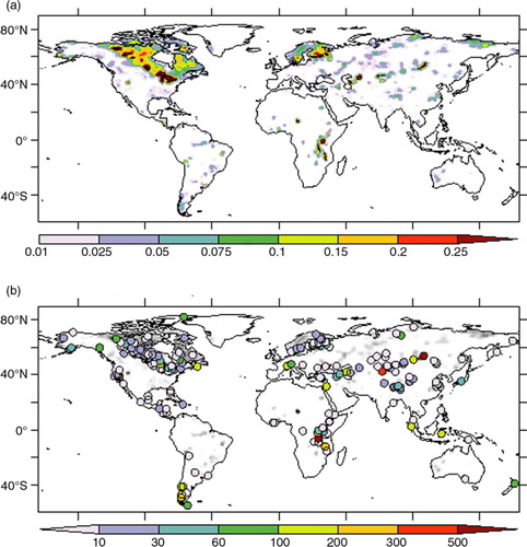
Two 32-yr long inline simulations (1979–2010) were carried out with the CNRM-CM5 climate model at a 30-min time step. This accounts for the physical and dynamical interactions between atmosphere, land surface and ocean (including sea-ice) as described in detail by Voldoire et al. (2013). In this study, it is used in forced mode, meaning using prescribed AMIP (Atmospheric Model Intercomparison Project) monthly mean sea surface temperature (SST; www-pcmdi.llnl.gov/projects/amip/AMIP2EXPDSN/BCS_OBS/amip2_bcs.htm) instead of interactive ocean and sea-ice numerical schemes. In the first simulation, the FLake scheme is activated wherever 1 % or more of the grid cell's surface corresponds to a lake in the ECOCLIMAP database. The resulting fraction of lake in each cell is shown in Fig. 1. In order to assess the impact of the modelling of lakes in the CNRM-CM5 model, another inline simulation was performed without FLake. In this case, all lake surfaces are treated in the same way as the surrounding land areas.

Fig. 1 (a) Fraction of lake cover (%) in CNRM-CM5. (b) Location and depth of the 200 selected lakes for the ARC-Lake database.

In CNRM-CM5, the atmospheric physics and dynamics are described using the global spectral ARPEGE-Climat model. ARPEGE-Climat is derived from the ARPEGE/IFS (Integrated Forecast System) numerical NWP model developed jointly by Météo-France and the European Center for Medium-Range Weather Forecast. The atmospheric physics and dynamics are solved on a reduced T127 triangular truncation Gaussian grid equivalent to a spatial resolution of about 1.4° in both longitude and latitude. In CNRM-CM5, ARPEGE-Climat uses a low-top configuration with 31 vertical levels that extend from the surface to 10 hPa in the stratosphere following a progressive hybrid r-pressure discretisation. The model uses physical parameterisations for deep and shallow convection and includes six prognostic variables: temperature, specific humidity, ozone concentration, logarithm of surface pressure, vorticity and divergence. The detailed description of all atmospheric components is given in Voldoire et al. (2013).

The land surface processes are simulated via the ISBA (Interaction Soil-Biosphere-Atmosphere) land surface model embedded into the SURFEX platform. ISBA uses the so-called force-restore method to calculate the time variation of the surface energy and water budgets via a composite soil–vegetation–snow approach (Noilhan and Planton, 1989). The snowpack evolution is based on a simple one-layer scheme following Douville et al. (1995). ISBA used a three-layer hydrology in which a rooting layer includes a thin surface layer (1 cm depth), while an additional layer is used to distinguish between the rooting depth and the total soil depth (Boone et al., 1999). Only the two uppermost layers can freeze/thaw according to atmospheric and soil temperature conditions using an explicit freeze–thaw scheme (Boone et al., 2000). Finally, a comprehensive parameterisation of subgrid hydrology is also included to account for the spatial heterogeneity of precipitation, topography, soil properties and vegetation within each grid cell (Decharme and Douville, 2006, 2007).

3.3. Evaluation data sets

To evaluate both offline and inline simulated lake surface temperatures, we used observations given by the ARC-Lake project (MacCallum and Merchant, 2013; www.geos.ed.ac.uk/arclake/). ARC-Lake is funded by the European Space Agency to characterise lake water surface temperatures and ice cover from remote-sensed data. Measurements are performed with ATSR1-2 (Along Track Scanning Radiometers) radiometers and AATSR radiometers onboard ERS1-2 or ENVISAT satellites to provide continuous measurements from 1991 to 2010 for major lakes at the global scale. Such satellites have a quasipolar orbit and are earth synchronous, ensuring homogeneity in the measurements, since they fly over the same lakes at the same solar time. The surface temperature measurement errors were estimated to range from −0.2 K to +0.7 K. The database products were used to evaluate the quality of the offline simulations. We focused on large lakes that cover an area greater than 500 km². Among the 263 lakes available in the database, 63 were not selected because they cover less than 20 % of the mesh's fraction when the model is run at the resolution of the atmospheric forcing (half a degree). Figure 1 shows the location of the 200 largest selected lakes, and Appendix B.1 lists their main characteristics: latitude, longitude, altitude and depth. The daily mean of the ARC-Lake surface temperature was compared to the daily averaged model output only when the observed surface temperature was greater than 0 °C, as no measurements were available over frozen or snow-covered lakes. However, this allows the number of days when a lake is frozen to be computed and compared to the number of frozen days simulated by the model.

To evaluate inline simulations, we also compared the simulated monthly mean of daily minimum and maximum 2 m air temperatures against observation from the Climatic Research Unit (CRU) version 3.22 (Harris et al., 2014). This product consists of a gridded climate data set from monthly observations at meteorological stations across the world's land areas. The original data at 0.5° resolution have been set to the CNRM-CM5 resolution (~1.4°) using a bilinear interpolation.

4. Offline calibration

Five simulations are performed offline to evaluate the calibration of FLake parameters and are then summed up in Table 1. First, a reference simulation, hereafter denoted as XPR, using lake depths from ARC-Lake was conducted. The 60-yr spin-up duration was evaluated from the XPR experiment, for which lake depths were the largest and, therefore, represent an upper bound duration for the other experiments where lake depths were reduced. To evaluate the impact of depth limitation at the global scale, a twin experiment, named XPD, was driven where depth was limited to 60 m. Figure 1 shows the position of the 200 selected lakes, and the evaluation is based on the 30 m which have a depth greater than 60 m (corresponding to coloured spots in Fig. 1) and present over all continents. The results in terms of surface temperature are presented in Fig. 2. Four lakes were selected for their geomorphologic contrasts and for the various climates they experienced. These lakes are Lake Superior (Fig. 2a), one of the American Great Lakes, Lake Baikal (Fig. 2b) in south Siberia, Lake Malawi (Fig. 2c) in East Africa and Lake Buenos-Aires (Fig. 2d) in Patagonia, with real depths of 150, 680, 273 and 290 m, respectively. In each of these figures, the surface temperature mean annual cycle from ARC-Lake (solid line with full circles) referenced as observations (OBS hereafter), XPR (dotted line with empty circles) and XPD (dashed line with crosses) are presented. The first remarkable feature is that limiting depth enhances the annual cycle amplitude in most cases. In the model, a lake will distribute the energy received over its total height. Decreasing this height will lead to an average warming of the lake. The seasonal averages DJF and JJA are improved significantly (see Table 2) for Superior and Malawi (DJF and JJA) and for Baikal (JJA) in XPD as compared to XPR. DJF cannot be evaluated for frozen lakes because OBS is not available in winter. Such an improvement is not always experienced; for example, the limitation of the depth for Lake Buenos-Aires, which already exhibits a good annual cycle in the XPR simulation, leads to an over-warming during DJF and an over-cooling during JJA. Figure 2e and f shows the differences between XPR minus XPD of the absolute bias and the root mean square error (RMSE) of the surface temperature, respectively. Very strong biases are reduced with XPD, but depending on the location, intermediate biases of about ±0.5 K can be reduced or increased by limiting the lake depth. However, the difference in RMSE shows that most of the time XPD leads to a reduction in the error, with the largest model error occurring in South America.

Fig. 2 Impact of depth limitation on the mean annual cycle of surface temperature: (a) Lake Superior, (b) Lake Baikal, (c) Lake Malawi, (d) Lake Buenos-Aires, (e) map of biases difference XPR minus XPD and (f) map of RMSEs difference XPR minus XPD.

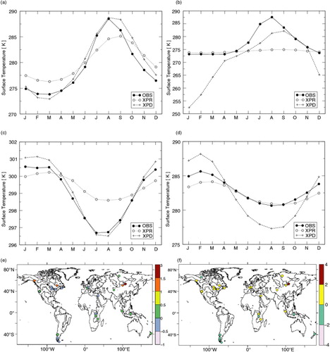
Table 1. Summary of offline calibration experiments

Exp.	Max depth (m)	Ice albedo	Light extinction coefficient (m^−1)	Skin temperature
XPR	Unlimited	0.6	3.0	On
XPD	60	0.6	3.0	On
XPA	60	0.4	3.0	On
XPE	60	0.4	0.5	On
XPF	60	0.4	0.5	Off

Table 2. Comparison of seasonal biases for XPR and XPD for four selected lakes

	DJF		JJA
Lakes	XPR	XPD	XPR	XPD
Baikal	/	/	−8.7	−5.5
Superior	2.6	0.3	−1.9	0.7
Malawi	−0.5	0.5	1.8	−0.0
Buenos-Aires	−1.5	1.9	0.1	−3.0

Lakes Superior, Malawi and Buenos-Aires are never frozen, leading to an annual cycle in phase with OBS. The presence of ice and snow over Lake Baikal is responsible for a shift in the simulated temperature as compared to OBS, as the FLake scheme has a tendency to produce too much ice.

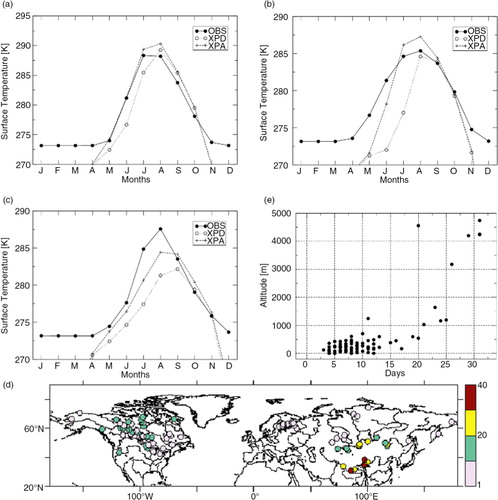
The ice albedo has been reduced from 0.6 to 0.4 to diminish the delay between the break-up observed by satellite and the one derived from the model simulations. This approach was motivated by the fact that in the presence of both ice and open water, satellites measure a composite albedo, which can be assumed to be the average of ice albedo close to 0.71 and water albedo close to 0.07. On average, a 0.4 albedo was chosen to represent the real lake albedo. The offline simulation accounting for this decreased albedo was named XPA, and the proposed change consists of darkening the lake ice significantly. The direct consequence of such a modification was evaluated for the lakes that froze in winter. Figure 3a–c shows the annual cycle of surface temperature for Lake Athabasca in Canada, Ngoring on the Tibetan Plateau and Baikal. The shape of the annual cycle is similar for these three lakes, with a melting delay ranging from a few days to a month. XPA reduced the delay as compared to XPD; consequently, the open water warmed earlier, leading to a higher maximum during summer. A generalisation of this result is shown in Fig. 3d, highlighting the melting delay for all 200 lakes: a minimum reduction of 2 d and a maximum of 32 d were found. In most cases, the delay reduction ranges between 2 and 12 d, but for lakes with an altitude greater than 1000 m, the reduction is far higher, with the Tibetan plateau exhibiting the highest biases. Figure 3e clearly shows that there is a dependence on the delay with height, and above 1000 m the delay is generally reduced by more than 20 d in XPA.

Fig. 3 Impact of ice albedo reduction on mean annual cycle of the surface temperature: (a) Lake Athabasca, (b) Lake Ngoring, (c) Lake Baikal, (d) map of reduction of thaw delay (days) for XPD minus XPA and (e) map of reduction of thaw delay as a function of height.

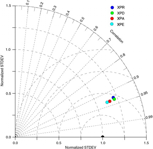
In FLake, part of the incoming solar radiation I ₀ is reflected by the surface characterised by its albedo α, and another part of the radiation penetrates the water body. The attenuation of light with depth follows a Beer–Lambert (Bouguer, 1729; Lambert, 1760; Beer, 1852) law that writes I(z)=(1 − α)I ₀exp(−k∣z∣), where k is the extinction coefficient of light with the default value of 3 m⁻¹ in the model. For example, over open water (α=0.065), only 46 W/m² will reach the first water meter for a solar energy supply of 1000 W/m², which is commonly observed at mid-latitudes during summer time. Such an extinction coefficient corresponds to a turbid water body. Sensitivity tests of the simulated surface temperature to the extinction coefficient were performed to try to optimise this coefficient, and the consideration of clear lakes was shown to improve the results for nearly all lakes. For that reason, a coefficient of 0.5 m⁻¹ was chosen, and a new experiment named XPE was carried out to demonstrate the improvement associated with this change. Figure 4 is a Taylor diagram that summarises the four experiments described above. All lakes have been gathered into one, and global statistics were computed. In Fig. 4, the blue circle corresponds to XPR, the green circle to XPD, red to XPA and cyan to XPE. The improvement induced by XPD was discussed previously and is illustrated by a better correlation in the Taylor diagram. XPD, XPA and XPE have nearly the same correlation, close to 0.94, and the normalised error equals 0.44, 0.41 and 0.39, respectively. XPE is found to be the optimal configuration for an application at the global scale.

Fig. 4 Taylor diagram summarising the improved surface temperature results for experiments XPR, XPD, XPA and XPE.

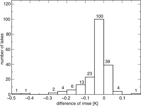
The final step is to verify that the use of the skin temperature parameterisation leads to improved results; the XPE experiment was chosen for this purpose. A final model configuration with this option turned off was designed, and the experiment was called XPF. Figure 5 shows a histogram of the surface temperature RMSE comparing XPE and XPF. Although the impact of the activation of a skin temperature parameterisation is limited to a few tenths of centimetres, results show that for most lakes the surface temperature RMSE is smaller for XPE than XPF, proving that XPE performs better than XPF and confirming the positive impact of such a parameterisation.

Fig. 5 Histogram of RMSE differences of surface temperatures XPE minus XPF for which skin temperature parameterisation has been turned off.

5. Offline versus inline experiments

In this section, the XPE offline simulation is compared to inline simulations. This offline simulation is now referenced as Offline-FLake. The two inline simulations using CNRM-CM5 (see Section 3.2) with and without FLake are now referenced as Inline-FLake and Inline-noFLake, Inline-FLake having the same setup as XPE.

5.1. Evaluation of Offline-FLake and Inline-FLake experiments

The evaluation relies on the ARC-Lake data set. Since these data are bounded at 0 °C, we consider only the positive values when computing the differences between the model and the observations. Therefore, in high latitudes, the winter temperatures of the lakes cannot be evaluated, and they are not taken into account in mean annual statistics. We can, however, compare the number of days for which each lake is frozen (later referred to as ‘frozen days’).

As we can see in Fig. 6, the mean annual surface temperature bias of Offline-FLake is generally positive. Further analysis shows that it is stronger in summer than in the other seasons (not shown). In the offline simulation, it remains inferior to 2–3 °C for most of the 200 lakes. It is stronger in the inline simulation, Inline-FLake, where the bias can reach 4 to 5 °C for some lakes in North America. This reflects the atmospheric bias of the climate model (not shown). The number of frozen days is fairly well captured in Offline-FLake, especially in the highest latitudes, with relative differences below 20 %. In Canada, the differences are generally negative, meaning that in the Offline-FLake, the ice sheets hold for a shorter time period, whereas the opposite is true in Scandinavia and over the Great Lakes. The magnitude of errors is greater in the mountainous areas of Eastern Europe, central and Eastern Asia. In these regions, the Offline-FLake can simulate up to twice too many frozen days compared to the observations. Inline-FLake exhibits the same patterns with stronger biases – which still remain below 20 % – in northern Canada and Scandinavia. Figure 7 shows the mean annual cycle of surface temperature for 12 lakes whose characteristics are listed in Table 3. Here, the performances of Offline-FLake vary quite a lot depending on the lakes. However, the errors generally stay below 5 °C. Lakes Nicaragua, Tai and Taymyr have their annual cycle almost perfectly captured. For Lakes Victoria, Tahoe and Great Bear, the Offline-FLake shows a systematic positive bias ranging from 1 to 4 °C. The Aral Sea and Lakes Constance, Baikal and Lagoda are too cold in spring and summer (with 2 to 5 °C biases), whereas during fall their simulated temperature is either correct or slightly too high – which is also the case for Lake Superior. Also, in Offline-FLake the Aral Sea is frozen in winter, which is unrealistic according to the ARC-Lake data set. Overall, Inline-FLake basically shows the same behaviours with more pronounced errors. For the lakes that freeze in winter, the simulated amplitude of the seasonal cycle is stronger than it is in Offline-FLake.

Fig. 6 Evaluation of Offline-FLake and Inline-FLake versus ARC-Lake data. Top: Mean annual surface temperature (°C) of lakes. Bottom: Number of days per year (%) for which each lake is frozen. Left panel: Offline-FLake – ARC-Lake. Right panel: Inline-FLake – ARC-Lake.

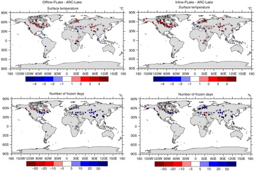
Fig. 7 Mean annual cycles of surface temperatures (°C) over 12 lakes whose characteristics are given in Table 3. Black line: ARC-Lake data; blue line: Offline-FLake; and red line: Inline-Flake.

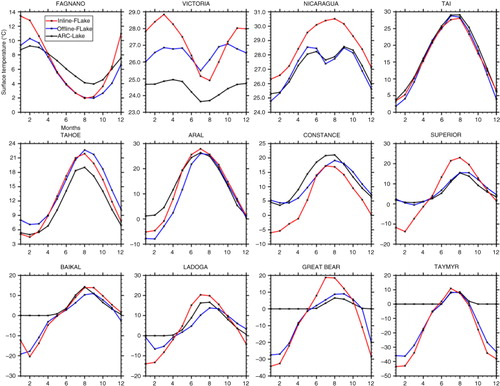
Table 3. Characteristics of lakes

	Latitude	Longitude	Altitude (m)	Mean lake depth (m)
Fagnano	−54.55	−68.03	169	70
Victoria	−1.30	33.23	1140	40
Nicaragua	11.57	−85.36	31	13
Tai	31.21	120.24	2	2
Tahoe	39.09	−120.04	1996	249
Aral	45.13	60.08	42	16
Constance	47.65	9.28	431	90
Superior	47.72	−88.23	184	149
Baikal	53.63	108.14	450	680
Ladoga	60.84	31.39	11	52
Great Bear	65.91	−121.30	157	72
Taymyr	74.48	100.76	24	3
Malawi	−11.96	34.59	485	273
Buenos-Aires	−46.66	−72.50	451	290
Ngoring	34.93	97.71	4240	18
Athabasca	59.10	−109.96	212	26

5.2. Impact of the modelling of lakes in CNRM-CM5

In the CNRM-CM5 climate model, the representation of lakes mainly affects the thermodynamic variables – moisture and temperature – in the lower layers of atmosphere. The impact of lakes varies depending on the region and the season. Figures (8–10) delve into the differences in surface and 2 m air temperatures between Inline-FLake and Inline-noFLake. The first two columns of Fig. 8 show the differences in surface temperature and albedo over the lakes’ surfaces – albedo can have a significant impact on the temperature when there is snow and/or ice on the lakes. For Inline-FLake, we consider the variables computed by FLake on the fraction of the grid cell corresponding to a lake, whereas for Inline-noFLake we take the compound value computed by SURFEX on the whole grid cell. In this way, we can isolate the effects of the presence of lakes. Then, we consider the total surface temperature in both simulations (i.e. the weighted mean of all types of surfaces in the grid cell), as this is the end result, which is shown in the third column of Fig. 8. In Figs. 9 and 10, we plotted the differences of daily minimum and maximum 2 m air temperatures between the two simulations, along with their biases compared to the CRU data. Differences of the simulated 2 m specific humidity, latent and sensible heat flux are shown in Fig. 11. All values are seasonally averaged.

Fig. 8 Seasonal mean differences with and without FLake (Inline-FLake – Inline-noFLake) of Albedo and surface temperatures (°C). Left panel: Surface albedo over lakes. Central panel: Surface temperature over lakes. Right panel: Total surface temperature.

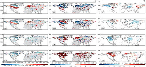
Fig. 9 Seasonal mean daily maximum 2-meter temperature (°C). Left panel: Inline-noFLake – CRU. Central panel: Inline-FLake – CRU. Right panel: Inline-FLake – Inline-noFLake. The grey-stippled areas on the right panel indicate a 95 % significance.

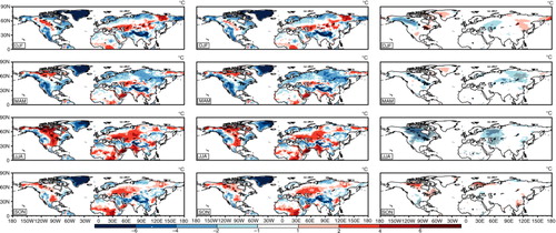
Fig. 10 Same as Fig. 9 for daily minimum 2-m temperature.

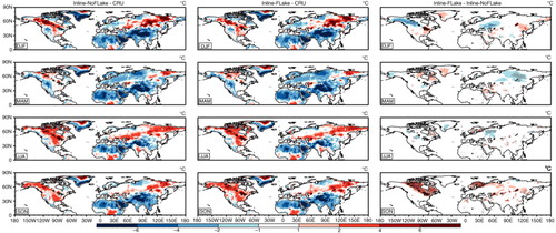
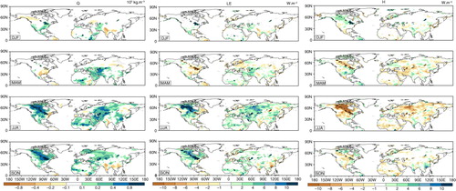
Fig. 11 Seasonal mean differences with and without FLake (Inline-FLake – Inline-noFLake) of specific humidity (10³ kg/m³) on the left panel, latent heat flux (W/m⁻²) on the central panel and sensible heat flux (W/m⁻²) on the right panel. The grey-stippled areas indicate a 95 % significance.

In winter, the representation of lake surfaces has a different impact if the lake water is frozen or not. When lakes remain free of ice whereas the surrounding surfaces are frozen and/or partially covered with snow, the surface temperature is increased with the use of FLake; this is, for example, the case in the Great Lakes area (Fig. 8, central and right panels). Given the size of these lakes, they store too much heat in the warmer seasons to freeze in winter. When there is ice and snow on the lakes, the effect of simulating them depends on the kind of land surface they replace. In tundra regions, as the low vegetation is almost completely covered with snow, the presence of lakes has a limited impact. In this case, changes between Inline-FLake and Inline-noFLake could emerge from FLake's snow scheme and/or from the differing snow albedos over lakes and land surface (it is set to 0.6 in FLake whereas it varies in ISBA). According to Fig. 8, in the tundra regions, the albedo over lake surfaces is lower in Inline-FLake but the difference does not lead to higher lake surface temperatures in Inline-FLake. On the contrary, these are lower (Fig. 8, central panel) but it does not impact the total surface temperature which is averaged over all types of surfaces (Fig. 8, right panel). Over the taiga regions, icy lakes covered with snow replace darker forestry land surfaces, thus exhibiting higher albedos. This may contribute to the cooling of surface temperatures occurring in Canada and Alaska (Fig. 8, central and right panel), at least in the southern part of this area – where there would be enough lakes and enough solar radiation for the albedo to play a role. However, changes in larger scale processes may also be involved, as for instance a reduced flux coming from the Pacific Ocean (not shown) in Inline-FLake whose exact cause is hard to establish. All the significant differences in surface temperature in winter are transmitted to both the minimum and maximum 2 m air temperatures, and they all correspond to an improvement of the CNRM-CM5 model with the representations of lakes surfaces with FLake (Figs. 9 and 10).

During the spring, there is still an important snow cover in the tundra regions. As in winter, the albedo computed over lake surfaces is lower in Inline-FLake (Fig. 8, left panel). But this time, with the increase of the daylight duration in spring, this leads to a significant warming of the surface temperatures over the lake surfaces (Fig. 8, central panel). However, this effect is no longer significant once we consider the total surface temperatures (Fig. 8, right panel) and the 2 m air temperatures (Figs. 9 and 10). Further down south, over the Great Lakes in Canada and in the lake region of Finland, the snow has partially melted on the land surfaces but the lakes have not thawed yet (not shown), as FLake does not simulate partially thawed lakes. Thus, the lake's albedo is higher than the land surfaces, and this results in colder surface temperatures in Inline-FLake (Fig. 8, right panel) which can be also seen on the maximum 2 m air temperature (Fig. 9). Where there is neither snow nor ice on lakes, the temperature can still be lower in Inline-FLake, as for example over the Great Lakes. This behaviour is, thus, similar to that which is observed in summer. In this season, the representation of lakes with FLake tends to slightly deteriorate the results, except in northern Canada, where it constitutes a small improvement.

In summertime, the main impact of the modelling of lake surfaces is a significant cooling of the daily maximum 2 m air temperatures over the Great Lakes, a large part of Canada, western Russia and, to a lesser extent, in the region located east of the Caspian Sea (Fig. 9). As these areas are affected by a fairly strong warm bias in summer, the impact of FLake is clearly positive here. The processes involved are quite simple. During the day, the lakes’ surfaces are cooler than the surrounding continents (Fig. 8), the sensible heat flux is thus reduced and the atmosphere is less heated by the surface (Fig. 11). There is also a contribution of the increased latent heat flux, due to a significant increase in evaporation above the lakes during the day. Over Scandinavia and Quebec, representing lake surfaces with FLake has an opposite effect. In these regions, lakes have a warming effect at night, instead of the daytime cooling previously described. This can be explained by the reduced solar radiation simulated by the model over these regions (not shown). The presence of lakes does not have a cooling influence because the continental surfaces are less heated during the day. At night, however, the land surfaces become colder than the lakes (as they did not receive much heat during the day), and in this case lakes warm up the lower layers of the atmosphere. In both cases, the presence of lakes locally weakens the diurnal cycle whether it is through a cooling of relatively high maximum temperature or a warming of relatively low minimum temperatures.

In autumn, the presence of lakes clearly has a warming and moistening role. The increase in temperature mainly affects Canada and Scandinavia. The mechanism is similar to that of summer, but here it also applies during the day, albeit with less strength. In parallel, the humidity and latent heat flux are stronger in Inline-FLake almost everywhere that there are lakes, but this does not prevent the warming. In Scandinavia, where Inline-noFLake is too cold, the biases are reduced by FLake, but elsewhere, the increase in temperature degrades the results.

To assess the vertical structure of FLake's possible impacts on the simulated climate, we now consider vertical slices of potential temperature and specific humidity. Figure 12 shows the seasonal mean differences (Inline-FLake minus Inline-noFLake) of these two variables for three vertical slices over the following regions: the Canadian tundra (120°W–100°W/60°N–70°N), the Canadian taiga (150°W–110°W/55°N–65°N) and the Great Lakes (95°W–75°W/42°N–50°N). These regions were chosen to illustrate the various effects of FLake. The slice is zonal in the taiga and meridian in the two other boxes.

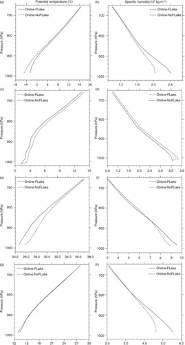
Fig. 12 Meridian and zonal slices of potential temperature (°C) and specific humidity (10³ kg/m³) differences (Inline-Flake – Inline-noFLake) over the following three boxes: Canadian tundra (120°W–100°W/60°N–70°N), Canadian taiga (150°W–120°W/55°N–65°N) and Great Lakes (95°W–75°W/42°N–50°N). (a) Winter (DJF); (b) summer (JJA); and (c) autumn (SON).

In winter (Fig. 12a), we can observe the three different behaviours that were previously identified: few effects on the tundra, cooling and drying over the taiga (in our box, it is mostly located over the mountains) and warming and moistening over the Great Lakes. The differences are visible up until 700 hPa for temperature and up to 850 hPa for humidity. In summer (Fig. 12b), the cooling and moistening differences exhibit roughly the same vertical extension. The summer increase of minimum temperatures observed in Quebec and Scandinavia cannot be seen on any vertical slice, indicating that this effect of the presence of lakes remains confined to the surface (it is not contradictory with the fact that it did show on the 2 m minimum temperature (Fig. 9) because the 2 m temperature is a diagnosis involving the surface temperature). During the spring (not shown), the differences are either small or limited to the lowest levels. In autumn (Fig. 12c), the warming does not propagate upward to a significant extent. The moistening effect, on the other hand, does reach 850 hPa.

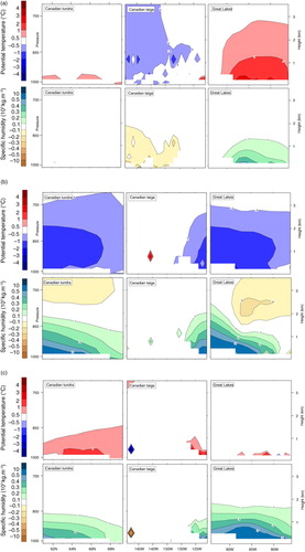
Overall, four different types of changes induced by FLake emerge. They are summarised in Fig. 13, which represents the four typical vertical profiles of seasonal mean humidity and potential temperature:

• winter in a cold region above a non-frozen lake (Fig. 13a and b): increase in both temperature and moisture up to 850 hPa,

• winter above a frozen lake in an evergreen forest region with snow (Fig. 13c and d): moderate decrease in temperature and moisture up to 700 hPa,

• summer in a relatively warm region (Fig. 13e and f): decrease in temperature and increase of moisture up to 800 hPa,

• autumn (Fig. 13g and h): slight increase in temperature in the lowest levels (up to 925 hPa) and significant moistening up to 800 hPa.

Our analysis shows that in winter, the two main effects of FLake constitute an improvement in the CNRM-CM5 model. This is also the case for the summer cooling of temperatures. Only the warming occurring in autumn leads to less realistic air temperatures in eastern Canada and Scandinavia. Therefore, the overall impact of FLake is quite positive.

Fig. 13 Typical vertical profiles of potential temperature (°C) (a, c, e, g) and specific humidity (10³ kg.m⁻³) (b, d, f, h). (a) and (b) correspond to the winter (DJF) mean over Lake Michigan; (c) and (d) are the winter means (DJF) over south Alaska (145°W–130°W/56°N–61°N); (e) and (f) are the summer (JJA) mean over Lake Michigan; (g) and (h) are the autumn (SON) means over Lake Michigan.

6. Discussion and conclusion

Results indicate that FLake satisfactorily simulates the lake surface temperature in offline mode. Although the bias for most of the 200 lakes is generally larger than 1 °C (Fig. 6), it remains lower than 2–3 °C. This rather large range may not be entirely attributed to the FLake scheme. The ERA-I atmospheric forcing is based on an atmospheric reanalysis in which small lakes are generally unresolved while larger lakes are combined with the surrounding land surface. Therefore, for a majority of the 200 lakes simulated locally, ERA-I represents an atmospheric state which is certainly warmer and dryer than that above free water. This can partly explain the general positive bias simulated by FLake for most of the 200 lakes. The choice to use ERA-I instead of other global forcing data sets (Sheffield et al., 2006; Weedon et al., 2011) was motivated by a better consistency between the analysed atmospheric variables than for other global forcings.

When coupled with the CNRM-CM5 model, FLake shows larger errors than in offline mode, as it inherits the atmospheric biases. However, these errors remain acceptable (<4° in most cases). Of course, there is always room for future improvements, but our analysis shows that FLake can now be used successfully within a climate model.

In CNRM-CM5, the changes induced by FLake on the simulated climate are rather limited and, most of the time they are local and confined to the lower levels of atmosphere as expected. Mainly, the modelling of lakes with FLake leads to a significant reduction in the summer warm bias of the 2 m temperature over Canada. It also lessens the warm bias simulated in winter over the Great Lakes of Canada. On the other hand, it produces a warm bias on the daily minimum 2 m temperatures in Canada in autumn. These changes can be explained by physical processes which involve the modifications of surface albedo, water content and heat storage capacity of the surface, which can have an impact on the atmosphere through radiative fluxes, evaporation and heat fluxes.

The impact of FLake might be more visible at a higher resolution, as more grid points will have a higher lake cover. With the T127 truncation used in our study, the fraction of lake is rarely above 0.25. And since the surface fluxes are averaged over the different tiles present in the mesh (in our case: nature, sea and lake), the atmospheric model mostly ‘sees’ nature over the lake areas. With smaller meshes, there would be more grid points for which the surface is mostly composed of lakes; and therefore, more cases where the atmosphere would be fed with surface fluxes mostly computed by FLake.

The choice of some FLake parameters, such as extinction coefficient and snow/ice albedo, can appear debatable. In this study, the extinction coefficient of the solar radiation in the water is, for all lakes, representative of clear water. However, tropical lakes are usually turbid media with a large amount of suspended solid matter and, therefore, a large extinction coefficient. An increase in this coefficient in such regions would lead to a warming of the water at surface due to the reduction of the solar penetration into the deepest layers. A tuning method could have been applied for each lake or over each region, but such a tuning is certainly not advisable at the global scale, since it could hide some atmospheric forcing or model deficiencies. The same remark applies for the choice of the snow (0.6) and ice (0.4) albedo, which can seem a bit low. During break-up periods, the albedo of lakes is gradually representative of snow, a mixing of snow and ice, a mixing of ice and water and finally only water. During this transition phase from ice to water, the surface is composed of water and ice and the real albedo is a combination of both. Nevertheless, these values allow compensation for a weakness of the model due to an overly simple parameterisation of the snow processes over lakes. During winter, the FLake snow scheme does not succeed in isolating the lake ice cover efficiently enough. For that reason, the simulated ice thicknesses are too large, leading to iced periods which are too long (Figs. 3 and 6). Such a weakness is reduced by the choice made for the snow and ice albedo.

The comparison of FLake versus CROCUS has demonstrated that the snowpacks simulated by FLake were not thick and insulating enough compared to those simulated by CROCUS (not shown). We expect an improvement of the snowpack simulations by coupling FLake to the more physical snow model ISBA-ES used in SURFEX (Decharme et al., 2016). This study is a prerequisite to the simulation of the water budget of lakes in FLake and more generally in the hydrologic or climatic applications at the global scale, and will contribute to improving the simulation of the continental water cycle.

7. Acknowledgements

This work was supported by the ‘Centre National d'Etudes Spatiales’ (CNES) within the framework of the SWOT satellite mission preliminary studies, the ‘Centre National de Recherches Météorologiques’ (CNRM) of Météo-France and the ‘Centre National de la Recherche Scientifique’ (CNRS) of the French research ministry.

8. Appendix

A.1. Skin temperature computation

As mentioned in Section 2.1, the objective was to solve the 1D heat transfer equation in a lake, where the total derivative of temperature T is in balance with the diffusion of temperature and a heat source Q due to the divergence of the net radiation flux at the surface. If ρ _w is the water density, c _w the water heat capacity at constant pressure and λ _w the water conductivity, this equation writes:A1

For a lake, Q can be simplified into the divergence of the solar radiation R neglecting the divergence of the long-wave radiation, which is a common assumption. At the continuum scale, decomposing an instantaneous field into an average denoted with an overlined bar plus a fluctuation denoted with a prime, applying the Reynolds averaging operator to eq. (A1) and using Einstein summation convention leads toA2

In the vicinity of the viscous layer, the turbulent term is negligible when compared to the diffusion term. If, on top of that, an assumption of horizontal homogeneity is applied to a steady state, eq. (A2) simplifies and writes:A3

which can be directly integrated between depth z and the surface:A4

The boundary condition at z=0 writes: , where L* is the net long-wave radiation, and QH and QE are the surface sensible and latent heat fluxes, respectively. According to the Beer–Lambert law:A5

By replacing this expression in eq. (A4), the following differential equation has to be solved:A6

where S* is the net short-wave radiation. Integrating eq. (A6) between z= − h and z=0 leads to the final expression of the skin temperature:A7

In this expression, L* + S* − QH−QE is the amount of heat transferred to the water body and is the FLake surface temperature computed as if no skin temperature parameterisation was applied.

B.1. Description of the 200 lakes used for the evaluation

LAKE	Lat (N)	Lon (E)	Height (m)	Depth (m)	Name
1	−54.55	−68.03	169	70	FAGNANO
2	−50.33	−73.03	225	150	ARGENTINO
3	−49.59	−72.56	297	75.8	VIEDMA
4	−48.75	−72.84	330	170	SAN MARTIN
5	−46.66	−72.5	451	290	BUENOS-AIRES
6	−45.47	−68.76	251	2	COLHUE HUAPI
7	−41.14	−72.79	56	182	LLANQUIHUE
8	−40.92	−71.52	810	157	NAHUEL HUAPI
9	−38.81	175.9	395	91	TAUPO
10	−35.52	139.09	20	2.8	ALEXANDRINA
11	−33.16	−52.84	8	3.95	MANGUEIRA
12	−30.74	−62.61	66	7.3	CHIQUITA
13	−18.81	−67.06	3679	0.5	POOPO
14	−15.32	35.71	629	2	CHILWA
15	−11.96	34.59	485	273	MALAWI
16	−8.71	29.72	945	2	CHISHI
17	−8.65	26.4	586	0.9	UPEMBA
18	−6.95	141.53	59	5	MURRAY
19	−6.07	29.46	837	572	TANGANYIKA
20	−3.58	35.04	1023	1	EYASI
21	−2.79	121.52	230	100	TOWUTI
22	−2.34	36.02	583	2.3	NATRON
23	−2.04	29.23	1500	240	KIVU
24	−1.3	33.23	1140	40	VICTORIA
25	−0.82	17.98	338	4	TUMBA
26	−0.39	29.61	781	34	EDWARD
27	1.5	33.01	1043	6	KYOGA
28	1.72	32.65	1043	6	KWANIA
29	2.61	98.9	898	184.6	TOBA
30	5.23	−3.23	73	3.8	ABY
31	5.3	−4.26	74	4.5	EBRIE
32	5.83	37.55	1249	6	CHAMO
33	6.3	37.83	1249	7	ABAYA
34	7.46	100.38	67	1	LUANG
35	11.17	41.79	414	8.6	ABE
36	11.57	−85.36	31	13	NICARAGUA
37	11.95	37.31	1786	8	TANA
38	12.32	−86.35	56	7.8	MANAGUA
39	12.54	−83.67	0	2.5	PERLAS
40	14.36	121.26	12	3	BAY
41	15.35	−83.85	0	5	CARATASCA
42	15.57	−89.11	47	12	IZABAL
43	18.49	−71.58	8	14	ENRIQUILLO
44	19.69	85.38	16	1.35	CHILKA
45	20.21	−103.05	1573	7.2	CHAPALA
46	21.66	−97.57	0	2	TAMIAHUA
47	24.64	−97.66	0	1.1	MADRE
48	26.95	−80.86	4	3	OKEECHOBEE
49	28.24	−80.64	0	0.9	INDIAN RIVER
50	28.97	90.76	4446	23.6	YAMDROK
51	30.71	90.66	4704	34	NAM
52	30.9	85.61	4743	4	TERINAM
53	31.05	86.59	4649	25	TANGRA
54	31.13	88.32	4640	15	KYARING
55	31.21	120.24	2	1.9	TAI
56	31.52	35.49	−404	149	DEAD
57	31.57	117.57	1	3	CHAO
58	31.77	88.95	4557	33	ZILING
59	32.87	119.31	1	7.9	GAOYOU
60	33.3	−115.83	−74	8	SALTON
61	33.34	118.53	3	1.4	HUNGTZE
62	33.82	78.61	4200	16	PANGONG
63	34.61	117.24	7	4.2	WEISHAN
64	34.92	97.27	4256	13.1	GYARING
65	34.93	97.71	4240	17.6	NGORING
66	35.25	136.08	69	41	BIWA
67	36.89	100.18	3176	17	QINGHAI
68	37.78	31.52	1148	5	BEYSEHIR
69	38.01	−118.96	1955	16.5	MONO
70	38.07	30.85	946	9	EGRIDIR
71	38.31	97.59	4239	4	HAR-HU
72	38.66	42.98	1638	57	VAN
73	38.7	−118.71	1339	24	WALKER
74	39.02	−122.77	474	6.5	CLEAR
75	39.09	−120.04	1996	249	TAHOE
76	40.03	−119.55	1161	60	PYRAMID
77	40.26	−121.19	1403	27.5	ALMANOR
78	40.39	45.29	1876	41	SEVAN
79	41.23	53.54	−22	10	KARA-BOGAZ-GOL
80	41.85	50.36	−22	182	CASPIAN
81	41.98	87.07	1062	9.7	BOSTEN
82	42.25	−81.16	174	19	ERIE
83	42.46	77.25	1619	320	ISSYKKUL
84	42.5	−82.73	174	3	SAINT CLAIR
85	43.34	−118.83	1242	0.6	MALHEUR
86	43.85	−77.77	75	86	ONTARIO
87	43.86	−87.09	176	85	MICHIGAN
88	44.02	−88.42	229	4.7	WINNEBAGO
89	44.45	−73.27	35	22.8	CHAMPLAIN
90	44.47	−79.42	233	15	SIMCOE
91	44.78	−82.21	176	59	HURON
92	44.83	28.97	1	3	RAZELM
93	44.86	82.92	166	1.5	EBI
94	45.13	60.08	42	16	ARAL
95	45.91	73.95	329	7	BALKHASH
96	45.95	−60.83	35	150	BRAS D'OR
97	45.96	34.74	2	1	SYVASH
98	46.11	81.75	336	22	ALAKOL
99	46.24	−79.92	212	4.5	NIPISSING
100	46.24	−93.65	381	6.4	MILLE LACS
101	46.26	42.98	15	0.6	MANYCH-GUDILO
102	46.37	6.25	466	154.4	GENEVA
103	46.58	80.91	342	3.3	SASYKKOL
104	46.88	17.83	126	4	BALATON
105	47.22	87.3	452	8	ULUNGUR
106	47.65	9.28	431	90	CONSTANCE
107	47.72	−88.23	184	149	SUPERIOR
108	47.81	117.69	597	8.1	BUYR
109	48.04	−95.08	358	9	RED
110	48.05	93.21	1160	4	HAR
111	48.06	92.3	1191	4	HAR US
112	48.61	−92.97	343	9.9	RAINY
113	48.66	−72.02	97	11.4	SAINT JEAN
114	48.97	117.38	539	5	HULUN
115	49.13	93.3	1027	20	HYARGAS
116	49.8	−88.55	283	54.9	NIPIGON
117	50.07	115.81	595	4.6	BARUN-TOREY
118	50.44	68.9	297	7	TENGIZ
119	50.82	−73.81	374	75	MISTASSINI
120	50.97	−77.02	231	5	EVANS
121	50.99	−98.8	247	12	MANITOBA
122	51.02	100.48	1640	138	HOVSGOL
123	51.27	−99.77	259	2.4	DAUPHIN
124	51.48	136.51	80	2.5	EVORON
125	52.12	−97.25	217	13	WINNIPEG
126	52.37	−100.05	252	4.24	WINNIPEGOSIS
127	52.98	79.58	92	3.9	KULUNDINSKOYE
128	53	−93.03	282	5.36	SANDY
129	53.22	−76.75	174	8	SAKAMI
130	53.23	73.18	66	1.9	SELETYTENIZ
131	53.33	−100.14	256	4.18	CEDAR
132	53.63	108.14	450	680	BAIKAL
133	53.77	−90.02	210	10.5	BIG TROUT
134	53.83	−100.04	256	4.1	SOUTH MOOSE
135	53.85	−94.7	230	20.1	ISLAND
136	54.05	−100.16	257	4.1	NORTH MOOSE
137	54.07	−97.75	217	4	PLAYGREEN
138	54.19	−64.31	472	4.3	SMALLWOOD
139	54.62	−94.21	181	13.2	GODS
140	54.71	−97.58	203	8.2	CROSS
141	54.76	−107.28	459	10.9	DORE
142	54.78	−103.45	329	6.2	DESCHAMBAULT
143	55.05	−72.98	423	13	BIENVILLE
144	55.11	−104.83	371	12.7	RONGE
145	55.43	−115.49	604	11.7	LESSER SLAVE
146	55.47	80.05	131	2	UBINSKOYE
147	55.84	−108.55	423	13.7	PETER POND
148	55.96	−108.29	423	9	CHURCHILL
149	56.15	−74.4	251	5.2	EAU CLAIRE
150	56.37	−108.22	423	5.5	FROBISHER
151	56.39	162.77	1	4.4	NERPICH'YE
152	56.78	9.17	3	7	LIMFJORDEN
153	57.19	−102.27	337	17	REINDEER
154	57.47	−106.64	484	14.9	CREE
155	57.85	−156.4	22	56	BECHAROF
156	58.3	−103.33	396	20.6	WOLLASTON
157	58.33	14.57	91	39	VATTERN
158	58.59	−112.08	212	1.2	CLAIRE
159	58.64	−155.67	39	41	NAKNEK
160	58.88	13.22	45	27	VANERN
161	59.1	−109.96	212	26	ATHABASCA
162	59.44	16.19	18	11.9	MALAREN
163	59.56	−154.9	35	44	ILIAMNA
164	59.57	−133.75	704	86	ATLIN
165	60.18	37.64	122	4.15	BELOYE
166	60.22	−115.49	264	2.8	BUFFALO
167	60.54	−117.64	277	1	TATHLINA
168	60.84	31.39	11	52	LADOGA
169	61	22.28	52	5.5	PYHAJARVI
170	61.09	25.39	96	6	VESIJARVI
171	61.37	−97.29	184	18	SOUTH HENIK
172	61.71	25.49	95	17	PAIJANNE
173	61.77	29.02	79	12	PURUVESI
174	61.9	35.35	56	30	ONEGA
175	62.09	−114.37	158	41	GREAT SLAVE
176	62.1	28.52	80	17	HAUKIVESI
177	62.35	29.59	79	17	ORIVESI
178	62.89	25.99	107	7	KEITELE
179	63.16	29.71	113	9.9	PIELINEN
180	63.17	−107.82	359	2.13	ARTILLERY
181	63.32	33.76	129	29	SEGOZERO
182	63.33	−117.91	265	9	MARTRE
183	63.54	34.84	74	7.4	VYGOZERO
184	63.93	−97.66	115	2.5	PRINCESS MARY
185	64.53	174.44	2	6.8	KRASNOE
186	64.54	−110.38	454	28	GRAS
187	64.55	−98.59	76	18	ABERDEEN
188	65.62	32.09	112	16	TOPOZERO
189	65.91	−121.3	157	71.7	GREAT BEAR
190	65.95	−99.4	150	6.1	GARRY
191	66.07	30.98	118	15	PYAOZERO
192	66.42	−70.28	30	20	NETILLING
193	66.51	−160.73	1	15	SELAWIK
194	67.79	−97.73	1	5.8	SHERMAN
195	68.36	91.18	54	73	KHANTAYSKOE
196	69.04	27.83	126	14.4	INARI
197	69.77	87.78	17	4	PYASINO
198	70.59	−153.6	0	1	TESHEKPUK
199	74.48	100.76	24	2.8	TAYMYR
200	81.8	−70.94	182	85	HAZEN

References

- Balsamo G., Salgado R., Dutra E., Boussetta S., Stockdale T., co-authors. On the contribution of lakes in predicting near-surface temperature in a global weather forecasting model. Tellus A. 2012; 64: 15829. DOI: http://dx.doi.org/10.3402/tellusa.v64i0.15829.
- Bartlett P., Lehning M. A physical SNOWPACK model for the Swiss avalanche warning: part I: numerical model. Cold. Reg. Sci. Technol. 2002; 35(3): 123–145. DOI: http://dx.doi.org/10.1016/s0165-232x(02)00074-5.
- Berrisford P., Kallberg P., Kobayashi S., Dee D., Uppala S., co-authors. Atmospheric conservation properties in ERA-Interim. Q. J. Roy. Meteorol. Soc. 2011; 137: 1381–1399. DOI: http://dx.doi.org/10.1002/Qj.864.
- Beer A . Bestimmung der Absorption des rothen Lichts in farbigen Flüssigkeiten [Determining the absorption of red light in colored liquids]. Annalen der Physik und Chemie. 1852; 86: 78–88.
- Best M. J. , Beljaars A. , Polcher J. , Viterbo P . A proposed structure for coupling tiled surfaces with the planetary boundary layer. J. Hydrometeorol. 2004; 5: 1271–1278.
- Bonan G. B . Sensitivity of a GCM simulation to inclusion of inland water surfaces. J. Clim. 1995; 8: 2691–2704.
- Boone A. , Calvet J.-C. , Noilhan J . Inclusion of a third soil layer in a land surface scheme using the force-restore method. J. Appl. Meteor. 1999; 38: 1611–1630.
- Boone A. , Masson V. , Meyers T. , Noilhan J . The influence of the inclusion of soil freezing on simulation by a soil-atmosphere-transfer scheme. J. Appl. Meteor. 2000; 9: 1544–1569.
- Bouguer P . Essai d'optique sur la gradation de la lumière [Optical essay on light gradation]. 1729; Paris: Claude Jombert. 16–22.
- Brun E. , David P. , Sudul M. , Brunot G . A numerical model to simulate snow-cover stratigraphy for operational avalanche forecasting. J. Glaciol. 1992; 38: 13–22.
- Brun E. , Martin E. , Simon V. , Gendre C. , Cole C . An energy and mass model of snow cover suitable for operational avalanche forecasting. J. Glaciol. 1989; 35: 333–342.
- Decharme B., Bruna E., Boone A., Delire C., Le Moigne P., co-authors. Impacts of snow and organic soils parameterization on northern Eurasian soil temperature profiles simulated by the ISBA land surface model. Cryosphere. 2016; 10: 853–877. DOI: http://dx.doi.org/10.5194/tc-10-853-2016.
- Decharme B. , Douville H . Introduction of a sub-grid hydrology in the ISBA land surface model. Clim. Dyn. 2006; 26: 65–78.
- Decharme B., Douville H. Global validation of the ISBA Sub-Grid Hydrology. Clim. Dyn. 2007; 29: 21–37. DOI: http://dx.doi.org/10.1007/s00382-006-0216-7.
- Dee D. P., Uppala S. M., Simmons A. J., Berrisford P., Poli P., co-authors. The ERA-Interim reanalysis: configuration and performance of the data assimilation system. Q. J. Roy. Meteorol. Soc. 2011; 137: 553–597. DOI: http://dx.doi.org/10.1002/qj.828.
- Douville H. , Royer J.-F. , Mahfouf J.-F . A new snow parameterization for the Météo-France climate model. PartI: validation in stand-alone experiments. Clim. Dyn. 1995; 12: 21–35.
- Downing J. A., Prairie Y. T., Cole J. J., Duarte C. M., Tranvik L. J., co-authors. The global abundance and size distribution of lakes, ponds, and impoundments. Limnol. Oceanogr. 2006; 51: 2388–2397. DOI: http://dx.doi.org/10.4319/lo.2006.51.5.2388.
- Dutra E. , Stepanenko V. M. , Balsamo G. , Viterbo P. , Miranda P. M. , co-authors . Global offline lake simulations: validation and impact on ERA-interim. Boreal Environ. Res. 2010; 15: 100–112.
- Faroux S., Kaptué Tchuenté A. T., Roujean J.-L., Masson V., Martin E., co-authors. ECOCLIMAP-II/Europe: a twofold database of ecosystems and surface parameters at 1 km resolution based on satellite information for use in land surface, meteorological and climate models. Geosci. Model Dev. 2013; 6: 563–582. DOI: http://dx.doi.org/10.5194/gmd-6-563-2013.
- Garrett A. , Kurzeje R. , O'steen B. , Parker M. , Pendergast M. , co-authors . Observations and model predictions of water skin temperatures at MTI core site lakes and reservoirs. Proc. SPIE. 2001; 4381: 225–235.
- Harris I., Jones P. D., Osborn T. J., Lister D. H. Updated high-resolution grids of monthly climatic observations – the CRU TS3.10 dataset. Int. J. Climatol. 2014; 34: 623–642. DOI: http://dx.doi.org/10.1002/joc.3711.
- Jordan R . A One-dimensional Temperature Model for a Snow Cover (91-16). 1991; US Army Corps of Engineers Cold Regions Research and Engineering Laboratory, Hanover, NH.
- Kitaigorodskii S. , Miropolski Y . On the theory of the open-ocean active layer. Izv. Atmos. Ocean. Phys. 1970; 6(2): 178–188 (English edition).
- Kourzeneva E . External data for lake parameterization in numerical weather prediction and climate modeling. Boreal Environ. Res. 2010; 15: 165–177.
- Lafore J. P. , Stein J. , Asencio N. , Bougeault P. , Ducrocq V. , co-authors . The Meso-NH atmospheric simulation system. Part I: adiabatic formulation and control simulations. Ann. Geophys. 1998; 16: 90–109.
- Lambert J. H . Photometria, sive de mensura et gradibus luminis, colorum et umbrae [Photometry, or measurement of light intensity, colors and shadows] Sumptibus Vidae Eberhardi Klett. 1760
- Lehner B. , Döll P . Development and validation of a global database of lakes, reservoirs and wetlands. J. Hydrol. 2004; 296(1–4): 1–22.
- Le Moigne P. , Boone A. , Belamari S. , Brun E. , Calvet J.-C. , co-authors . SURFEX Scientific Documentation. 2012. Technical Report, Centre National de Recherches Météorologiques, Toulouse, France.
- Le Moigne P., Legain D., Lagarde F., Potes M., Tzanos D., co-authors. Evaluation of the lake model FLake over a coastal lagoon during the THAUMEX field campaign. Tellus A. 2013; 65: 20951. DOI: http://dx.doi.org/10.3402/tellusa.v65i0.20951.
- Lofgren B. M . Simulated effects of idealized Laurentian Great Lakes on regional and large-scale climate. J. Clim. 1997; 10: 2847–2858.
- MacCallum S. N., Merchant C. J. ARC-Lake v2.0, 1991-2011 [Dataset]. 2013; School of GeoSciences/European Space Agency: University of Edinburgh. Online at: http://hdl.handle.net/10283/88.
- Masson V. , Champeaux J.-L. , Chauvin F. , Meriguet C. , Lacaze R . A global data base of land surface parameters at 1 km resolution in meteorological and climate models. J. Clim. 2003; 16: 1261–1282.
- Masson V., Le Moigne P., Martin E., Faroux S., Alias A., co-authors. The SURFEXv7.2 land and ocean surface platform for coupled or off-line simulation of earth surface variables and fluxes. Geosci. Model Dev. 2013; 6: 929–960. DOI: http://dx.doi.org/10.5194/gmd-6-929-2013. Online at: www.geosci-model-dev.net/6/929/2013/.
- Mironov D. V . Parameterization of Lakes in Numerical Weather Prediction. Description of a Lake Model. 2008; Offenbach am Main, Germany: Deutscher Wetterdienst. 41. COSMO Technical Report No. 11.
- Noilhan J. , Planton S . A simple parameterization of land surface processes for meteorological models. Mon. Weather Rev. 1989; 117: 536–549.
- Perroud M. , Goyette S. , Martynov A. , Beniston M. , Anneville O . Simulation of multiannual thermal profiles in deep Lake Geneva: a comparison of one-dimensional lake models. Limnol. Oceanogr. 2009; 54: 1574–1594.
- Salgado R. , Le Moigne P . Coupling of the FLake model to the SURFEX externalized surface model. Boreal Environ. Res. 2010; 15: 231–244.
- Samuelsson P. , Kourzeneva E. , Mironov D . The impact of lakes on the European climate as simulated by a regional climate model. Boreal Environ. Res. 2010; 15: 113–129.
- Sheffield J. , Goteti G. , Wood E. F . Development of a 50-yr high-resolution global dataset of meteorological forcings for land surface modeling. J. Climate. 2006; 19(13): 3088–3111.
- Simmons A. , Uppala S. , Dee D. , Kobayashi S . ERA-interim: new ECMWF reanalysis products from 1989 onwards. Newsletter 110 – Winter 2006/07. 2007; ECMWF. Reading, UK, 11 pp.
- Taylor J. P. , Edwards J. M. , Glew M. D. , Hignett P. , Slingo A . Studies with a flexible new radiation code. II: comparisons with aircraft short-wave observations. Q. J. Roy. Meteorol. Soc. 1996; 122: 839–861.
- Voldoire A., Sanchez-Gomez E., Salas y Mélia D., Decharme B., Cassou C., co-authors. The CNRM-CM5.1 global climate model: description and basic evaluation. Clim. Dyn. 2013; 40: 2091. DOI: http://dx.doi.org/10.1007/s00382-011-1259-y.
- Verpoorter C., Kutser T., Seekell D. A., Tranvik L. J. A global inventory of lakes based on high-resolution satellite imagery. Geophys. Res. Lett. 2014; 41: 6396–6402. DOI: http://dx.doi.org/10.1002/2014GL060641.
- Vionnet V., Brun E., Morin S., Boone A., Faroux S., co-authors. The detailed snowpack scheme Crocus and its implementation in SURFEX v7.2. Geosci. Model Dev. 2012; 5: 773–791. DOI: http://dx.doi.org/10.5194/gmd-5-773-2012.
- Weedon G. P., Gomes S., Viterbo P., Shuttleworth W. J., Blyth E., co-authors. Creation of the WATCH Forcing data and its use to assess global and regional reference crop evaporation over land during the twentieth century. J. Hydrometerol. 2011; 12: 823–848. DOI: http://dx.doi.org/10.1175/2011JHM1369.1.