Parametric Kalman filter for chemical transport models

Abstract

A computational simplification of the Kalman filter (KF) is introduced – the parametric Kalman filter (PKF). The full covariance matrix dynamics of the KF, which describes the evolution along the analysis and forecast cycle, is replaced by the dynamics of the error variance and the diffusion tensor, which is related to the correlation length-scales. The PKF developed here has been applied to the simplified framework of advection–diffusion of a passive tracer, for its use in chemical transport model assimilation. The PKF is easy to compute and computationally cost-effective than an ensemble Kalman filter (EnKF) in this context. The validation of the method is presented for a simplified 1-D advection–diffusion dynamics.

• data assimilation
• Kalman filter
• covariance dynamics
• parameterisation of analysis

View correction statement:

Corrigendum

1. Introduction

One of the foundations of data assimilation is based on the theory of Kalman filtering. Because of its computational complexity and the extent of required information for its implementation, the Kalman filter (KF) has long been recognised as not viable for large dimension problems in geosciences. Alternative formulations, based for example on ensemble methods, have been developed. The ensemble Kalman filter (EnKF) was developed by Evensen (1994). The numerous formulations of the sequential algorithm or its smoother version have also had an impact on the variational data assimilation where new algorithms now take advantage of adjoint-free formulation. Considering other ensemble strategies, like particle filter methods in their present formulation, the EnKF is very robust and is used for atmospheric data assimilation with a limited ensemble of few dozen members.

Beside all its advantages and these developments, EnKF-like algorithms are approximations. To yield accurate simulations in real applications require addressing several scientific and practical considerations (see for example the review of Houtekamer and Zhang, 2016). For instance, to limit the filter divergence, inflation (Anderson and Anderson, 1999) or cross-validation (Houtekamer and Mitchell, 1998) strategies need to be employed. Another issue is related to the sampling error. Small and moderate ensemble sizes induce spurious long distance correlations that can be damped by either: (1) using a static localisation strategy based, for example, on Schur product with a compact support function (Gaspari and Cohn, 1999; Houtekamer and Mitchell, 2001) or a dynamical localisation (Bocquet, 2016); (2) filtering of variances (Berre et al., 2007; Raynaud et al., 2009) and length-scale (Raynaud and Pannekoucke, 2013); or (3) taking advantage of covariance modelling (Hamill and Snyder, 2000; Buehner and Charron, 2007; Pannekoucke et al., 2007; Kasanický et al., 2015). Some of these issues and their solutions are actually application dependent. This is the case, for example, for sampling errors in atmospheric chemistry assimilation, where the localisation based on distance is not useful to address the issue of sampling noise between correlated chemical variables at the same location.

The computational resources required for the time propagation of error information that is actually needed seems to be highly ineffectively used. Ensemble of model integrations creates by default a sample covariance for each pair of model grid point. Yet, it is only during the observation update that localisation is applied and where only a fraction of these pair of sample covariances is used. Why spend so much computational resources in computing ensembles if in the end we eliminate a large part of the information they provide? This actually suggests looking for other strategies than ensembles to reduce the computation cost of a KF and that is what we propose here – a solution applicable to chemical transport models.

The idea emerged from a seminal observation made by R. Daley (pers. commun., 1992) that under advection the diagonal of an error covariance matrix (i.e. the error variance) is simply transported, that is, it remains on the diagonal of the error covariance matrix. This also implies that the error variance can be predicted without knowledge of the error correlation. This was formally demonstrated by Cohn (1993) for quasi-linear hyperbolic equations and used in the assimilation of atmospheric constituents by Ménard et al. (2000) and Ménard and Chang (2000) in a realistic context with model error estimation. By fixing the error correlation and dynamically evolving only the error variance, Khattatov et al. (2000) developed a simplified KF known as the suboptimal KF or sequential filter. In Khattatov et al. (2000) the initialisation of the error variance is restricted to modest size of observation vectors as it requires an explicit computation of the analysis error variance via a Choleski decomposition. Dee (2003) proposed a variant of this formulation that does not suffer from this limitation using a sequential processing of the observations. The computational simplification in the advection of the error covariance is in fact not limited to the variance (i.e. diagonal of the error covariance matrix), but is applicable to the whole covariance function, by transporting any pair of points of the error covariance along the characteristics of the flow. As emphasised by (Cohn, 1993), since the number of characteristics that is needed is equal to the number of grid point (N) of the transport model, the computational cost of the transport of the error covariance is of order N rather than order N×N as in a KF. This led to the development of a fully Lagrangian KF by Lyster et al. (2004). However, regular remapping of the Lagrangian trajectories is needed to avoid clustering of the Lagrangian particles. Several variants of this algorithm have been used in the assimilation of both tropospheric and stratospheric chemical transport problems (Lamarque et al., 2002; Eskes et al., 2003; Rösevall et al., 2007) and for a 30 yr reanalysis of stratospheric ozone (Allaart and Eskes, 2010) which demonstrates the robustness of the algorithm. Despite these successful applications, the suboptimal KF filter does not account for diffusion, and the computation of the analysis error variance is done explicitly, which can be computationally demanding.

Recent works have paved the way for the parametric propagation of the error covariance matrix without ensemble, relying on the time evolution of the error variance and the length-scales or the associated diffusion tensor (Pannekoucke et al., 2014, 2016). The full covariance matrix and its propagation can be elaborated from a parametric covariance model, for example, covariance model based on the diffusion or the coordinate change. However, and as far as we know, the impact of reducing a KF to the propagation of error variance and length-scales has not been examined.

At first glance, the reduction of the error covariance matrix propagation, to the propagation of its error variance and its local correlation shape, may seem a crude approximation, but it is in fact not very different from variational data assimilation where these two ingredients are effectively used as initial conditions for the implicit propagation of the error covariance. Yet, in 4D-Var, the final error covariance is generally not used to initialise the next assimilation cycle. However, in the parametric Kalman filter (PKF), the final error covariance is used to feed the next assimilation cycle. Hence, the PKF presents the advantage of producing a cycle similar to the KF.

In this work, we propose a new algorithm that details the propagation of both the analysis variance and diffusion tensor for a linear advection–diffusion process. The algorithm also updates these error covariance parameters as a result of the observation update, that is, how the error variance and the diffusion tensor are modified after the assimilation of one observation and the iteration of this update. We limit our investigation to the case of linear advection–diffusion equation considered as a simple and robust description of the transport of chemical species. This way, the work is oriented towards the application of chemical transport model assimilation.

In Section 2, we review the description of the KF algorithm, with a particular focus on the background covariance matrix diagnostics and modelling. The assimilation of a single observation is presented, leading to the iterative assimilation of a collection of observations. Then, the PKF is detailed in Section 3, providing the algorithms associated with the analysis and the forecast cycle. In Section 4, a numerical validation of the PKF is proposed within a simple 1-D advection–diffusion setting. The conclusions of the results and further directions are provided in Section 5.

2. Insight with the one observation experiment

2.1. Kalman's equations

The aim of data assimilation is to estimate the true state of a dynamical system, , at a time t _q from the knowledge of observations, , and a prior state, . In this notation, the time is indicated by the subscript q. A simplified description of data assimilation is the following:

The observational operator, H _q (assumed linear here), maps the state vector onto the observational space, so that , where is an observational error which is often modelled as a Gaussian random vector of zero mean and covariance ( is the expectation operator), denoted by . The true state is unknown and the information about its possible value is modelled by a Gaussian probability distribution centred on a prior state and of covariance matrix B _q , denoted by . Put differently, the background error is a Gaussian random vector of zero mean and covariance , denoted by . The way we estimate the state of the truth can be formalised by using the Bayes’ rule , where p(·) denotes the probability density function. In the particular Gaussian setting, and for linear operators, the a posteriori density is also Gaussian and centred on the analysis state, with covariance matrix A _q , which verify the Kalman's analysis equations (Kalman, 1960)1

where K _q is the gain matrix. If the system evolution is governed by a linear dynamics, M _q+1←q , then the updated background statistics are Gaussian, featured by the forecast step Kalman's equations2

Thereafter, we focus on one analysis and forecast cycle, and the subscript q is dropped for the sake of simplicity.

In this formalism, eqs. (1) and (2) are the Kalman's equations for the covariance dynamics. This can be summarised by3

where . Note that the time evolution of the error covariance matrices does not involve the analysis state and so does the prior state in this case, where only linear operators are considered. Moreover, in the extended KF, occurs for the computation of the tangent linear propagator M _q+1←q . In real applications, these two steps are too numerically costly to be implemented as described by Eq.(2) and Eq.(3).

2.2. Description and modelling of correlation matrix

From a practical point of view, the potentially large size of the background error covariance matrix limits its full description in favour of simple local characteristics such as the grid point variance and the local shape of the correlation function.

For a normalised error where is the background error standard deviation at point x ; the correlation between two points, x and y , is defined as the ensemble expectation . The shape of a smooth correlation function ρ ^b ( x , y ) with respect to a grid point x can be described with the metric tensor field defined as . Hence, the Taylor expansion of the correlation function ρ ^b ( x , x +δx ), denoted by ρ ^b _x (δx ), reads4

where , and f= _ao(g) means . Note that the formalism can be enlarged to other correlation functions, for example, the exponential functions (Pannekoucke et al., 2014).

In practice, the local metric tensor g ^b _x can be estimated from an ensemble either from the computation of the correlation coefficient in the vicinity of x (Pannekoucke et al., 2008) or from the covariance of partial derivative of the error (Daley, 1993, p. 156; Belo Pereira and Berre, 2006) whose practical computation takes the form (see Appendix A)5

This formulation of the metric tensor is particularly adapted to the derivation of analytical length-scale properties, for example, the sampling error statistics (Raynaud and Pannekoucke, 2013).

More than a simple diagnosis, the local metric tensor has been considered as a simple way to set a background error covariance model. For instance, in the background covariance model based on the diffusion equation (Weaver and Courtier, 2001), Pannekoucke and Massart (2008) have proposed to relate the unknown local diffusion tensor to the local metric tensor. Since this particular covariance model is important for what follows, we detail this particular formulation.

The background covariance model, based on the diffusion equation, corresponds to the decomposition of the covariance matrix B as the product6

where L denotes the linear propagator. Hence, for a given field α and a diffusion tensor field ν, L is the time integration of the pseudo-diffusion equation7

from to , with a pseudo-time; hence, L is the abstract operator . Here the term ‘pseudo’ means that the diffusion is not related to a physical process but is only used as a trick to build Gaussian-like correlation functions. In the particular case where the diffusion tensor field is homogeneous and for initial condition α( x )=δ( x ) where δ stands for the Dirac distribution centred on zero, the particular Green solution on the real plane is given by the Gaussian function8

where ∣·∣ denotes the matrix determinant and .

Hence, the covariance model based on the diffusion allows constructing heterogeneous correlation functions design from the specification of the local diffusion tensor ν _x . However, in real application, the appropriate diffusion tensor remains unknown. To overcome this situation, Pannekoucke and Massart (2008) have proposed to connect the local diffusion tensor with the local metric tensor according to . Since the metric tensor can be deduced from an ensemble method, this allows an objective establishing of the diffusion tensor.

For a 1-D setting, the metric tensor takes the form , where denotes the background error correlation length-scale at position x. This length-scale is related to the diffusion coefficient by .

2.3. Assimilation of a single observation

The analysis error associated with the assimilation of an observation located at x _j can be deduced from the Kalman's analysis equation [see eq. (1)] by subtracting the truth on both sides of the equation, giving ɛ ^a=ɛ ^b+K(ɛ ^o − Hɛ ^b)when introducing the errors , and , and thus9

where denotes the covariance function associated with the grid-point x _j with and standing, respectively, for and the background error variance, . Thereafter, the background, the analysis and the observational variances are denoted, respectively, by V ^b , V ^a and V ^o .

From eq. (9), the two important covariance parameters, namely the variance field and length-scale field, can be computed (see Appendixes B and C). The error variance is10

This is a classical result of optimum interpolation (Daley, 1993, pp. 146–147) and its derivation in Appendix B appears only for the sake of completeness.

To facilitate the analytical derivation of the length-scale, an additional assumption of local homogeneity is introduced: for the background variance fields, we assume that locally, while is not globally constant or . After some calculations, detailed in Appendix C, it results that the local metric tensor is given by , in terms of diffusion tensor, since , this is also written as11

For the particular 1-D case, the update of the length-scale L ²=2ν takes the form12

where a second-order approximation of the length-scale update is given by (see Appendix C)13

This last formulation is much more complex than the leading order approximation [eq. (12)], but can be considered for simple numerical experiment.

From the description of the statistical update of the background variance [eq. (10)] and diffusion tensor [eq. (11)], when assimilating a single observation, we are now ready to describe the complete analysis and forecast cycle with several observations.

3. Parametric covariance dynamics along analysis and forecast cycles

The time propagation of covariance matrix has been studied by Cohn (1993) with real application in chemical transport model (CTM) by Ménard et al. (2000). However, these algorithms did not include the effect of diffusion, although some ideas on how to include it were discussed in Cohn (1993). This time propagation has been simplified under a parametric formulation (Barthelemy et al., 2012; Pannekoucke et al., 2014, 2016). In the present contribution, we fill the gap by including the effect of analysis and of diffusion in the whole assimilation cycle. But for completeness the whole algorithm will be described. This leads to a parametric formulation of the analysis and of the forecast steps, and will be called parametric Kalman filter (PKF).

3.1. Formulation of the analysis step

For the KF analysis step, with linear observational operator, the assimilation of multiple observations is equivalent to the iterated assimilation of single observations with an update of the covariance statistics (Dee, 2003).

Since the real correlation functions are unknown, the basic assumption made in the PKF is to assume a particular shape for the correlation functions, simple enough to be used in large dimension data assimilation systems, for example, isotropic correlations (based on spectral space diagonal assumption, anisotropic if diagonal in wavelet space), or Gaussian and Mattern's functions with the diffusion formulation (Mirouze and Weaver, 2010).

The Gaussian approximation for ρ _j can be used as an illustration of an analytic formulation leading to a simplified version of the correlation function14

where and . Another interesting aspect with Gaussian correlation function is its link with the Green solution [eq. (8)] of the diffusion [eq. (7)] with homogeneous diffusion tensor. Note that the Gaussian is the first-order approximation to the solution of the heterogeneous diffusion equation with slow spatial variations of the diffusion tensor field. Hence, we expect that the result of an analysis procedure, considering the analytic Gaussian correlation, would produce a solution close to the one deduced by using a background correlation matrix modelled with the diffusion equation (see Section 2.2), that is, the analysis variance and local diffusion tensor fields should be equivalent at the leading order.

Note that since the update process acts only on variance and metric fields, the approximation of the correlation function ρ _j by a Gaussian does not break the constraint of symmetry and positiveness of the resulting analysis-error covariance matrix, even if the collection of Gaussian functions does not form a proper correlation matrix. This represents a real advantage of this technique.

Algorithm 1 Iterated process building analysis covariance matrix at the leading order, under Gaussian shape assumption.

Require: Fields of ν ^b and V ^b , V ^o and location x _j of the p observations to assimilate

for j=1: p do

0-Initialisation of intermediate quantities

1-Computation of analysis statistics

2-Update of the background statistics

end for

Return fields ν ^a and V^a

Hence, the analysis covariance statistics can be computed following Algorithm 1. This takes advantage of the equivalence between analysis steps, considering all observations and an iterated analysis process where each observation is assimilated provided an inline analysis covariance matrix, featured by V ^a and ν ^a fields, and then uses an update of the background-error covariance.

In practice, the algorithm is parallelised following the same update as the one often used in the EnKF, that relies on batch of observations (Houtekamer and Mitchell, 2001): iteratively assimilating distant observations is equivalent (to a good approximation) to the assimilation at the same time. Note that the algorithm of Houtekamer and Mitchell (2001) relies on the compact support property of the correlation functions. A similar algorithm based on compact support property could have been considered here by using eq. (4.10) in Gaspari and Cohn (1999), whose shape is close to the Gaussian correlation. But, since the value of a Gaussian function is close to zero for large , we considered the correlation null beyond a distance of few length-scales.

3.2. Formulation of the forecast step

We consider the dynamics of a passive chemical tracer whose concentration α is governed by the linear advection–diffusion15

where u denotes the wind field. Since the dynamics is linear, the error dynamics is governed by the same equations, that is16

Starting from the initial condition , the matrix form of the covariance dynamics is given by17

where M _τ denotes the linear propagator associated with the time integration of eq. (16) from t=0 to t=τ.

The aim is to determine the time evolution of the principal diagnostic of the covariance matrix: the variance and the local diffusion tensor. So, as specified, it is not easy to formulate these two components and we propose to do this through a time-splitting. This time-splitting will lead to a tractable elementary evolution. Note that time-splitting is widely used in atmospheric chemistry (see, for example, Sportisse, 2007). In this study, the splitting goes beyond the numerical aspects, since it is employed to separate each processes (diffusion, advection) so as to simplify their analytical treatments. This helps to provide either a Lagrangian or an Eulerian formulation of the statistics dynamics. The forecast step proposed for the PKF results from these manipulations.

3.2.1. Time-splitting strategy for the covariance dynamics.

For short time integration δt, a time-splitting scheme can be used (Lie-Trotter formula), where M _δt is expanded as the product18

denotes the propagator, over [0, δt], associated with the pure advection ∂ _t ɛ ^b + u · ∇ ɛ ^b =0, and denotes the equivalent propagator associated with the pure diffusion ∂ _t ɛ ^b =∇· ( κ ∇ ɛ ^b ).

Hence, starting from B ₀=A, the time evolution of the background covariance matrix is then given as and approximated as19

This two-step covariance evolution can be analytically computed under some reasonable approximations.

3.2.2. Background error variance and diffusion field evolution associated with a pure advection.

The advection over a small time step δt can be viewed as equivalent of the deformation of the error field ɛ ^b under the action of the transformation D( x )= x + u ( x , t)δt (Pannekoucke et al., 2014). Hence, it follows that the metric tensor field g _x (t) evolves in time as , where D _x is the gradient deformation associated with D at x , and D ⁻¹ denotes the reversal deformation [Pannekoucke et al., 2014, see eq. (35)]. In terms of diffusion tensor (reminding that ),20

The variance resulting from a pure advection remains constant along the characteristic curve which results in21

3.2.3. Background error variance and diffusion field evolution associated with a pure diffusion.

The second step consists of a pure diffusion acting on the covariance dynamics. This is similar to the background covariance model based on the diffusion equation B=LL ^T [eq. (6)], but this time the pseudo-diffusion eq. (7) is replaced by a physical diffusion, , wherein we consider the diffusion of an existing Gaussian function: this can be viewed as a first time integration with a given diffusion tensor field leading to , followed by a time integration with another diffusion tensor field [the one given by κ ( x )].

We make the assumption that the diffusion is locally homogeneous [κ( x ) is locally constant], and approximate the covariance function in by local Gaussian functions22

Since diffusion is self-adjoint, the two diffusion time integrations act on the covariance as23

where ∣·∣ denotes the matrix determinant, and with24

Hence, the variance field resulting from the time evolution of the covariance matrix under the pure diffusion is given by25

while the diffusion tensor field is given by eq. (24).

3.2.4. PKF forecast step.

Algorithm 2 Iteration process to forecast the background covariance matrix at time t=τ from the analysis covariance matrix given at time t=0, under local homogenity assumption.

Require: Fields of ν ^a and V ^a . δt=τ/N, t=0

for k=1: N do

1-Pure advection

2-Pure diffusion

3-Update of the background statistics

end for

Return fields and

Combining the results of the two previous subsections, we obtain the forecast step of the PKF: from an initial analysis covariance matrix A diagnosed by the variance field and the diffusion field , the forecast step provides the variance and the diffusion tensor fields resulting from the time integration of the linear advection–diffusion equation eq. (15) from time t=0 to t=τ. The time propagation is provided by Algorithm 2.

3.2.5. Eulerian version of the PKF forecast step.

Note that Algorithm 2 is well suited for Lagrangian numerical solution (or at least semi-Lagrangian) since it implies the departure point D ⁻¹( x ), but an Eulerian version of this algorithm can also be written. From a combination of eqs. (20), (24), (21) and (25), it results (see Appendix D) that the Lagrangian algorithm 2 is equivalent to the integration over the range [0,t] of the Eulerian-coupled system of equations26

with the initial conditions given by and , and driven by the wind field u , and where Tr(·) denotes the matrix trace operator. This result is consistent with the model error-free version of eq. (4.32) described by Cohn (1993) who has considered the case of an advection process without diffusion ( κ =0) [see also eq. (5.26) in Cohn (1993) for the 2-D case] and has partially considered the case with diffusion. The originality of the present contribution is to provide another route toward the results of Cohn (1993) and fill the gap by considering the diffusion case.

The Eulerian description offers a nice change of view on the statistical dynamics. Under this form, it is easier to build a regularization of the dynamics. For example, this can be done by incorporating a nudging term that maintains the statistics close to a climatology so to prevent from the divergence of the statistics during long term runs. Another example is to incorporate a model error: following Cohn (1993), for model error given as a Gaussian random field, this would add the model error variance in the right side of variance equation, and add the model error local diffusion tensor in the right side of the diffusion tensor. Moreover, the Eulerian description provides implementation advantages in Eulerian numerical model, but it is less numerically efficient than a semi-Lagrangian implementation. In the sequel, only the Lagrangian version is considered.

3.2.6. Numerical cost of the PKF forecast step.

From a numerical point of view, one of the main advantages of the PKF is its low cost: the forecast step only requires the time propagation of the variance field and the diffusion tensor field. The diffusion tensor is a symmetric 2×2 (3×3) matrix in 2-D (in 3-D); hence; there are only 3 (6) fields in 2-D (in 3-D), corresponding to the upper triangular components of the symmetric matrix. Thus, the forecast step describes the time evolution of 4 (7) fields in 2-D (in 3-D). Compared with the EnKF, where dozens of forecasts have to be computed during the time propagation of the error covariance matrix, the PKF only requires a single time integration, with few additional fields within the state vector (4 or 7 depending on the dimension of the problem).

Combining the parallel strategy described for Algorithm 1 (as employed in EnKF), and the time evolution of the few fields required for the time propagation in Algorithm 2 (with also parallel strategy for this propagation), the PKF appears as a low-cost procedure to describe the covariance dynamics over the analysis and forecast cycles.

4. Numerical experiments

This section aims at validating the PKF equations. Two experiments are considered: the validation of the analysis step (Section 4.1) and the validation of the analysis-forecast cycle (Section 4.2). The experiments are conducted within a simplified 1-D setting. The geometry of the domain is an Earth great circle discretised with n=241 grid points (the space resolution is then δx=166 km). The PKF analysis step (Algorithm 1) is done first, followed by the full PKF loop of analysis and forecasting applied on a linear advection–diffusion dynamics. These results are compared with the KF [eqs. (1) and (2)], whose direct computation is affordable in a low dimensional setting.

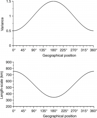
For the two experiments, the starting background covariance matrix is a heterogeneous covariance matrix, specified as follows. The variance field is chosen as varying from 0.5 near 0° to 1.5 near 180° (see Fig. 1, top panel). The background error correlation matrix is designed following the deformation example introduced in Pannekoucke et al. (2007). Here two choices of homogeneous correlation function are considered: the Gaussian and the second-order auto-regressive (SOAR) correlation functions. The homogeneous length-scale is set to L _h =500 km with a stretching of c=1.5 (see Pannekoucke et al., 2007, for details). The resulting background covariance presents a large length-scale area in the vicinity of 0° and a small length-scale area around 180° (see Fig. 1, bottom panel). In the weather framework, this choice mimics the situation where small length-scale areas are often the less predictable.

Fig. 1 Background error variance field (top) and length-scale field (bottom).

4.1. Validation of the analysis step

To test the analysis PKF step, we consider the assimilation of three observations located at 0°, 90° and 180°. The observational error variance is set to V ^o =1 for all these observations (crosses in Figs. 2 and 3, left panels).

Fig. 2 Illustration of analysis error variance (left panel) and length-scale (right panel) for the assimilation of three observations: 0, 45 and 90, when the background correlation is homogeneous and Gaussian. The Kalman reference (continuous line) is compared with the PKF analysis using the first-order eq. (12) (dash dotted line) and the second-order eq. (13) (dashed line).

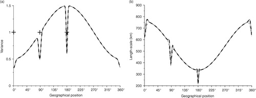
Fig. 3 Similar to Fig. 2 but when the background correlation is homogeneous and SOAR.

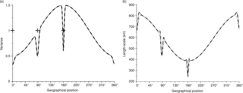
The analysis covariance matrix A resulting from eq. (1) has been computed and the diagnostic of its variance and length-scale fields are reproduced (continuous line) in Fig. 2 when the background error correlation is Gaussian and in Fig. 3 when it is the SOAR function. Assimilating observations in the system results in damping both the variance (left panel) and the length-scale fields (right panel). Since the distance between observations is large enough, their assimilations are deemed independent and three reduction peaks appear for each fields. For the length-scale, the reduction of the length-scale, at each observation locations, is accompanied by a local overshoot when compared with the initial background error length-scale field Fig. 1 (bottom panel).

The PKF analysis obtained from Algorithm 1 is reproduced in dash-dotted line. The resulting analysis variance field is superposed with the Kalman's reference (see left panels of Figs. 2 and 3). For the length-scale field, the local reduction due to the assimilation of each observation is approximately reproduced except the overshoot (see right panels of Figs. 2 and 3).

Replacing the approximation eq. (12) with the full formulation eq. (13) in the PKF algorithm (1) improves the approximation of the length-scale field (dashed line in right panels of Figs. 2 and 3). This does not modify the variance field that remains equivalent to the KF (see left panels of Figs. 2 and 3). It appears that, compared with eq. (13), eq. (12) provides a satisfactory representation of the length-scale update. This justifies the use of the first-order eq. (12) in Algorithm 1.

In the present experiment, the choice of the homogeneous correlation function used in the background covariance setting has no impact on the results. This is due to the fact that the discretised version of the Gaussian and the SOAR functions are not too different in this case.

The conclusion of this experiment is that the PKF as described in Algorithm 1 is able to reproduce the main feature of the analysis covariance matrix in terms of variance and length-scale fields. If a high-order formulation improves the PKF update of the length-scale, this remains costly for practical applications. Therefore, only the update proposed by Algorithm 1 is considered.

4.2. Covariance evolution over the analysis and forecast cycles within a simple linear advection–diffusion chemical model

To mimic situations encountered in chemical transport model, a simple advection–diffusion transport of a passive species is considered. The dynamics of the concentration α(x,t) is given by27

where c denotes the velocity and κ the diffusion rate. For the simulation, the velocity is set to c=1 and the time step dt is fixed to the advection time step δt _adv =δx/c. The diffusion rate is set so that the diffusion time step δt _diff =δx ²/κ is equal to six times the advection time scale dt _adv .

The observational network considered here is set to measure half the domain from 180° to 360°, with one observation per grid-point.

The initial background is assumed to be equivalent to the one described in the previous subsection. The correlations used are Gaussian (the homogeneous correlation length-scale is still fixed to 500 km).

The pure advection case (κ=0), in Fig. 4, and the full advection–diffusion case (κ>0), in Fig. 5, are successively considered. For the two situations, the results of the covariance dynamics as described from the KF equations are in continuous lines. The results obtained from the PKF analysis and forecast steps are reproduced in dashed line. The KF and the PKF can be compared with the update process proposed by Dee (2003) (see Ménard et al., 2000), thereafter called parametric homogeneous Kalman filter (PhKF), where only the variance is updated while the correlation function is isotropic and remains constant (dashed-dotted line).

Fig. 4 Diagnosis of the analysis covariance matrix at iterations 1 (a), 15 (b), 30 (c) and 60 (d) in case of a pure advection process. KF time evolution (continuous line), the PKF (dashed line) and the PhKF (dash dotted line).

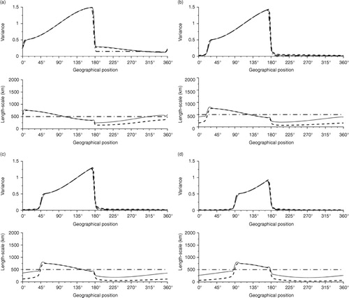
Fig. 5 Diagnosis of the analysis covariance matrix at iterations 1 (a), 15 (b), 30 (c) and 60 (d) in case of an advection–diffusion dynamics. KF time evolution (continuous line), the PKF (dashed line) and the PhKF (dash dotted line).

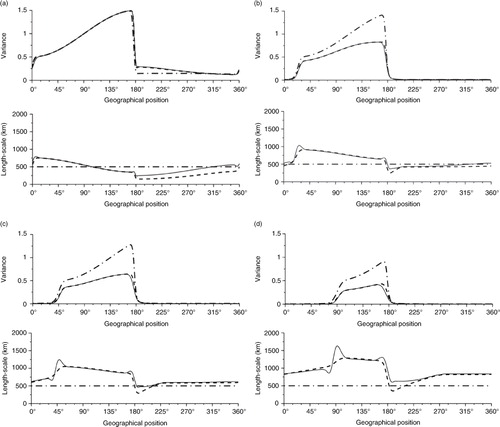
The pure advection (Fig. 4) shows that the two KF approximations lead to equivalent results. The PKF provides a better approximation of the KF equations than the Dee (2003) scheme.

The advantage of the PKF compared with the Dee (2003) scheme appears when the diffusion is switched on. For this case, the PKF is able to reproduce the variance attenuation due to the diffusion process, while the Dee (2003) scheme fails to reproduce the KF reference. Compared with the KF, the PKF is able to reproduce the time increase of the length-scale due to the physical diffusion term κ>0.

5. Conclusion

We have introduced the PKF, where a parametric representation of the error covariance is evolved through the analysis and the forecast steps of the KF. This applies to the advection–diffusion of a passive tracer considered here as a simplified version of chemical transport model. This parametric approach reduces to a description of the dynamics of the variance field and of the local diffusion tensor, when the covariance matrix is modelled with a diffusion equation. Compared with the classical KF forecast step, the numerical cost of the parametric forecast step is hugely reduced and in fact much cheaper than a typical EnKF implementation. In 2-D (in 3-D), only four (seven) fields are required to proceed for the time evolution: the variance field and the fields of the upper triangular components of the local symmetric diffusion tensor. The dynamics has been described under a Lagrangian and an Eulerian formulation.

The analytic formulation has been illustrated within a simple 1-D testbed where a passive tracer evolves through an advection–diffusion equation and is observed over a heterogeneous network. Compared with a full KF, the PKF shows that the parametric formulation is able to reproduce the main features of the real variance and of the real length-scale dynamics.

The main application of these results is to contribute to the development of robust data assimilation schemes for chemical transport models: with this formulation it is easy to evolve the background error covariance matrix at low numerical cost without an ensemble or localisation and yet account for flow-dependency. When chemistry is included, the PKF may actually become even more appealing, as the issue of localisation between species is no simple solution.

Beyond the application to chemical transport models, this parametric approach will certainly feed new developments in covariance localisation, which is an active field of research in data assimilation with the rise of ensemble-based four-dimensional variational data assimilation scheme. It also provides a simple framework for adaptive observation where the impact of new observations is approximated by using the parametric analysis step provided here. Further developments will be considered to incorporate, in part, non-linearities in the propagation process as well as to address the balance issue: the treatment of the simple linear advection–diffusion can be seen as the outline of the systematic description along the tangent-linear dynamics.

6. Acknowledgements

We would like to thank Emanuele Emili, Sebastien Massart and Daniel Cariole for fruitful discussions; Matthieu Plu for his comments on the manuscript; as well as Martin Deshaies-Jacques for revising the document.

7. Appendix A

A. Theoretical formulation of the metric tensor

In this section, and without loss of generality, the variance field is assumed to be homogeneous and equal to one. For smooth error field, the Taylor expansion, using Einstein's summation convention, writes . After multiplication by ɛ _x this leads to the correlation function

Since , the commutation rule and the homogeneity of the variance field imply that or . Similarly, by using the identity , the commutation rule and the homogeneity of the variance field lead to and then . Then, the Taylor expansion of the correlation takes the form

where from the identification with , it results that . In the general case where the variance of ɛ _x is not one, then the error is replaced by the normalised error that is of variance one, andA1

B. Derivation of analysis variance field

The analysis variance field is thus given by

With the classical assumption of observational error and background error decorrelation, it follows that and

The analysis variance then writesB1

C. Derivation of analysis length-scale field in 1D

Analysis length-scale at a given position x is given byC1

where , also written asC2

(where we have used and ).

Since the update of the analysis variance field, resulting from the assimilation of an observation located at grid-point x _j is given by eq. (10)C3

and the analysis error is given byC4

whereby the full computation of the analysis length-scale can be managed.

C.1. Derivation of length-scale formulation

In order to consider only the variance field, using , it follows that eq. (C2) takes the formC5

From eq. (C4), and using and , it results in

From

it follows that

Hence, the analysis length-scale writesC6

C.2. Derivation under local homogeneity assumption

To simplify the analytic derivation, a local homogeneity assumption is considered for the background error variance field.

This local homogeneity assumption for the background variance field means that _, while is not globally constant or

Hence, removing all spatial derivatives of σ ^b leads to the approximation of analysis length-scaleC7

Under local homogeneity assumption, the third term of the length-scale can be simplified: it can be shown that

leading toC8

C.3. Leading order and extension in dimension d

A crude, but simpler, approximation of the length-scale is obtained by removing all the partial derivative of the correlation function, leading toC9

that is exact in x=x _j (when is flat in x _j ).

From the last 1-D expression for the analysis length-scale, one can deduce that an approximation, in dimension d, of the analysis metric tensor defined by (in dimension d) is given byC10

where is the background error metric tensor at x defined by .

D. Derivation of the Eulerian version of the PKF forecast step

First, we combine the Lagrangian version of eqs. (20) and (24) to obtain the Eulerian version of the diffusion tensor field dynamics:

Since D=I+δt∇ u , eq. (20) writes leading to . But at leading order, D ⁻¹( x )= x − u ( x )δt and . Hence, combining in eq. (24), the infinitesimal dynamics of the diffusion tensor is given byD1

from which it results that the equivalent PDE isD2

Now, we combine eqs. (21) and (25) to obtain the Eulerian version of variance field dynamics.

By using the arguments first developed in the beginning of the previous paragraph, eq. (21) writesD3

The difficulty now is to replace the ratio of matrix determinant in eq. (25). Using the algebraic property that the determinant of two invertible matrices P and Q verifies ∣P ⁻¹ Q∣=∣Q∣/∣P∣, it follows thatD4

and from eq. (24), it follows that . Now the identity ∣exp (P)∣^1/2=exp (Tr(P)/2), where Tr denotes the matrix trace operator, implies at leading order thatD5

Hence, combining this last equation with eq. (21) implies the infinitesimal dynamicsD6

whose equivalent PDE is given byD7

From this analysis, it results that the Lagrangian algorithm 2 is equivalent to the integration over the range [0,τ] of the Eulerian-coupled system of equationD8

with the initial conditions given by and , and driven by the wind field u .

References

- Allaart M. A. F. , Eskes H. J . Multi sensor reanalysis of total ozone. Atmos. Chem. Phys. 2010; 10: 11277–11294.
- Anderson J. , Anderson S . A Monte Carlo implementation of the nonlinear filtering problem to produce ensemble assimilations and forecasts. Mon. Weather Rev. 1999; 127: 2741–2758.
- Barthelemy S. , Ricci S. , Pannekoucke O. , Thual O. , Malaterre P. O . Assimilation de donnees sur un modele d'onde de crue: emulation d'un algorithme de filtre de kalman. 2012; Sophia Antipolis. SimHydro 2012: Hydraulic Modeling and Uncertainty Online at: http://hal.cirad.fr/hal-01335907/document .
- Belo Pereira M. B. , Berre L . The use of an ensemble approach to study the background error covariances in a global NWP model. Mon. Weather Rev. 2006; 134: 2466–2489.
- Berre L. , Pannekoucke O. , Desroziers G. , Stefanescu S. E. , Chapnik B. , etal. A variational assimilation ensemble and the spatial filtering of its error covariances: increase of sample size by local spatial averaging. 2007; 151–168. ECMWF Workshop on Flow-Dependent Aspects of Data Assimilation, 11–13 June 2007, ECMWF, ed., Reading, UK.
- Bocquet M . Localization and the iterative ensemble Kalman smoother. Q. J. R. Meteorol. Soc. 2016; 142: 1075–1089.
- Buehner M. , Charron M . Spectral and spatial localization of background error correlations for data assimilation. Q. J. R. Meteorol. Soc. 2007; 133: 615–630.
- Cohn S. E . Dynamics of short-term univariate forecast error covariances. Mon. Weather Rev. 1993; 121: 3123–3149.
- Daley R . Atmospheric Data Analysis, Cambridge University Press. 1991; 471. 471.
- Dee D . An adaptive scheme for cycling background error variances during data assimilation. ECMWF/GEWEX Workshop on Humidity Analysis (July 2002). ECMWF. 2003
- Eskes H. J. , Van Velthoven P. F. J. , Valks P. J. M. , Kelder H. M . Assimilation of GOME total-ozone satellite observations in a three-dimensional tracer-transport model. Q. J. R. Meteorol. Soc. 2003; 129: 1663–1682.
- Evensen G . Sequential data assimilation with a nonlinear quasi-geostrophic model using Monte Carlo methods to forecast error statistics. J. Geophys. Res. 1994; 99: 10143–10162.
- Gaspari G. , Cohn S . Construction of correlation functions in two and three dimensions. Q. J. R. Meteorol. Soc. 1999; 125: 723–757.
- Hamill T. M. , Snyder C . A hybrid ensemble Kalman filter-3D variational analysis scheme. Mon. Wea. Rev. 2000; 128: 2905–2919.
- Houtekamer P. , Zhang F . Review of the ensemble Kalman filter for atmospheric data assimilation. 2016; 4489–4532. Mon. Wea. Rev. 144 .
- Houtekamer P. L. , Mitchell H. L . Data assimilation using an ensemble Kalman filter technique. Mon. Weather Rev. 1998; 126: 796–811.
- Houtekamer P. L. , Mitchell H. L . A sequential ensemble Kalman filter for atmospheric data assimilation. Mon. Weather Rev. 2001; 129: 123–137.
- Kalman R. E . A new approach to linear filtering and prediction problems. J. Basic Eng. 1960; 82: 35–45.
- Kasanický I. , Mandel J. , Vejmelka M . Spectral diagonal ensemble Kalman filters. Nonlin. Processes Geophys. 2015; 22: 485–497.
- Khattatov B. V. , Lamarque J.-F. , Lyjak L. , Ménard R. , Levelt P. , etal. Assimilation of satellite observations of long-lived chemical species in global chemistry transport models. J. Geophys. Res . 2000; 105: 29135–29144.
- Lamarque J.-F. , Khattatov B. V. , Gille J. C . Constraining tropospheric ozone column through data assimilation. J. Geophys. Res . 2002; 107: ACH 9-1–ACH 9-11.
- Lyster P. M. , Cohn S. E. , Zhang B. , Chang L. P. , Ménard R. , etal. A Lagrangian trajectory filter for constituent data assimilation. Q. J. R. Meteorol. Soc. 2004; 130: 2315–2334.
- Ménard R. , Chang L.-P . Assimilation of stratospheric chemical tracer observations using a Kalman filter. Part ii: chi-2-validated results and analysis of variance and correlation dynamics. Mon. Weather Rev. 2000; 128: 2672–2686.
- Ménard R. , Cohn S. E. , Chang L. P. , Lyster P. M . Assimilation of stratospheric chemical tracer observations using a Kalman filter. Part i: formulation. Mon. Weather Rev. 2000; 128: 2654–2671.
- Mirouze I. , Weaver A. T . Representation of correlation functions in variational assimilation using an implicit diffusion operator. Q. J. R. Meteorol. Soc. 2010; 136: 1421–1443.
- Pannekoucke O. , Berre L. , Desroziers G . Filtering properties of wavelets for local background-error correlations. Q. J. R. Meteorol. Soc. 2007; 133: 363–379.
- Pannekoucke O. , Berre L. , Desroziers G . Background error correlation length-scale estimates and their sampling statistics. Q. J. R. Meteorol. Soc. 2008; 134: 497–508.
- Pannekoucke O. , Emili E. , Thual O . Modeling of local length-scale dynamics and isotropizing deformations. Q. J. R. Meteorol. Soc. 2014; 140: 1387–1398.
- Pannekoucke O. , Emili E. , Thual O . Bélair J. , Frigaard I. A. , Kunze H. , Makarov R. , Melnik R. , Spiteri R. J . Modeling of local length-scale dynamics and isotropizing deformations: formulation in natural coordinate system. Mathematical and Computational Approaches in Advancing Modern Science and Engineering . 2016; Springer International Publishing. 141–151.
- Pannekoucke O. , Massart S . Estimation of the local diffusion tensor and normalization for heterogeneous correlation modelling using a diffusion equation. Q. J. R. Meteorol. Soc. 2008; 134: 1425–1438.
- Raynaud L. , Berre L. , Desroziers G . Objective filtering of ensemble-based background-error variances. Q. J. R. Meteorol. Soc. 2009; 135: 1177–1199.
- Raynaud L. , Pannekoucke O . Sampling properties and spatial filtering of ensemble background-error length-scales. Q. J. R. Meteorol. Soc. 2013; 139: 784–794.
- Rösevall J. D. , Murtagh D. P. , Urban J. , Jones A. K . A study of polar ozone depletion based on sequential assimilation of satellite data from the ENVISAT/MIPAS and Odin/SMR instruments. Atmos. Chem. Phys. 2007; 7: 899–911.
- Sportisse B . A review of current issues in air pollution modeling and simulation. J. Comp. Geosci. 2007; 11: 159–181.
- Weaver A. , Courtier P . Correlation modelling on the sphere using a generalized diffusion equation. Q. J. R. Meteorol. Soc. 2001; 127: 1815–1846.