The relationship between Indian summer monsoon rainfall and Atlantic multidecadal variability over the last 500 years

Abstract

Several studies have shown a statistically significant correlation between Atlantic multidecadal variability (AMV) and Indian summer monsoon rainfall (ISMR) since 1871 when instrumental data are available. In the instrumental records, both ISMR and North Atlantic sea surface temperatures (SSTs) have multidecadal variability with a period close to 60 yr, where periods of warm (cold) North Atlantic SSTs are accompanied by periods of wetter (dryer) ISMR and lower (higher) frequencies of dry years. We have studied both AMV and ISMR for the period from 1481 to present using several proxy reconstructions from both regions, as well as an extended instrumental data set for ISMR, to investigate multidecadal variability in the ISMR and the teleconnection to AMV. Previous studies investigating the relationship between AMV and ISMR in instrumental data have only used the period from 1871 onwards, whereas rain gauge data from the year 1844 are studied here, extending the instrumental record by 26 yr. We find that the observed link between AMV and ISMR is present in the extended instrumental data. We also find that multidecadal variability is present in the ISMR in all proxy records; however, all the proxy records for both ISMR and AMV diverge before the 1800s. In addition, the observed correlation between AMV and ISMR has weakened in the last decade. These results emphasise that it is not appropriate to use single proxy reconstructions to study past climates.

• Atlantic multidecadal variability
• Indian summer monsoon
• proxy reconstructions
• teleconnection
• multidecadal variability
• correlation analysis

1. Introduction

Multidecadal variability has been observed in Indian summer monsoon rainfall (ISMR) (Parthasarathy et al., 1994). The 4-month period from June to September constitutes the Indian summer monsoon season and gives about 78% of the mean annual rainfall of India (Mooley and Parthasarathy, 1984), with a standard deviation of about 10% of the mean. Parthasarathy et al. (1994) found that the measured rainfall data available from 1871 to present showed decadal departures of ISMR above and below the long-term average for 30-yr epochs. The years 1901–1930 and 1961–1990 were epochs with low decadal mean monsoon rainfall and frequent dry years, whereas the years 1871–1900 and 1931–1960 were epochs with high decadal mean monsoon rainfall and infrequent dry years (a dry year is defined as a year in which monsoon rainfall is lower than the mean by at least one standard deviation). This approximate 60-yr period is found to be in phase with Atlantic multidecadal variability (AMV) (Fig. 1; Goswami et al., 2006). The AMV is associated with basin-wide low-frequency sea surface temperature (SST) variability in the North Atlantic (Enfield et al., 2001) and has earlier been related to decadal variability in a number of regions, such as European and North American summer climate (Sutton and Hodson, 2005) and rainfall in African Sahel, as well as ISMR (Zhang and Delworth, 2006). A significant correlation between the observed AMV and ISMR suggests a link between these two regions. Here we investigate whether this link holds before the instrumental period by using several available annual-resolution proxy reconstructions.

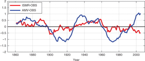
Fig. 1 Instrumental ISMR (red) and the AMV-index (based on Kaplan Extended SST V2 data) from June to September (blue) smoothed with an 11-yr moving average (1856–2010).

Several studies have investigated the teleconnection between AMV and ISMR based on observational data and modelling experiments (Goswami et al., 2006; Zhang and Delworth, 2006; Li et al., 2008; Luo et al., 2011). Goswami et al. (2006) showed that the AMV produced persistent weakening (strengthening) of the meridional gradient of tropospheric temperature by setting up a negative (positive) tropospheric temperature anomaly over Eurasia during the northern summer or autumn resulting in an early (late) withdrawal of the monsoon and a persistent decrease (increase) of seasonal monsoon rainfall. Zhang and Delworth (2006) suggested that during the positive AMV phase, the intertropical convergence zone over the Atlantic shifts northwards, resulting in anomalous southwesterly surface winds over India and Sahel, convergence of surface moisture and thus enhanced summer monsoon rainfall over India and Sahel. The positive AMV phase reduces sea level pressure over Asia and Europe and snow cover over Tibet, which, in turn, strengthens the monsoon rainfall over India. Luo et al. (2011) found that the influence of AMV on ISMR was achieved through an atmospheric teleconnection process in which a propagating Rossby wave train from the North Atlantic across South Asia enhanced the South Asia high. However, this relationship is not robust in coupled model simulations (Ting et al., 2011), and it is not clear whether this link on decadal timescales is causal and internal to the climate system, or specific for the observational time period.

A connection between ISMR and North Atlantic SST on centennial and millennial timescales has also been indicated, linking cold events in the North Atlantic to a weakening of the Asian monsoon during the Holocene and the last glacial period (Burns et al., 2003; Gupta et al., 2003). Similarly, Overpeck et al. (1996) found this linkage to be significant for glacial–interglacial cycles. Covariations between ice-core- and tree-ring-derived surface temperatures of the Tibetan Plateau, the ISMR and North Atlantic SSTs have also been found on interglacial timescales in proxy records covering the past 2000 yr (Feng and Hu, 2005, 2008). The proxy data used in these studies mostly have decadal-to-centennial temporal resolution.

The aim of our study is to investigate the relationship between decadal variability of ISMR and AMV extended over the past 500 yr (from 1481). Therefore, we have collected and analysed the available ISMR data using a combination of available high-resolution proxy records and rain gauge observations and compared with available AMV reconstructions. In Section 2, we analyse the available instrumental data of ISMR and AMV. Section 3 describes the proxy data used to estimate ISMR and AMV in this study. Decadal variability in the ISMR proxy reconstructions is assessed in Section 4 and compared with AMV reconstructions in Section 5. The results are discussed and summarised in Section 6.

2. Instrumental data of ISMR and AMV used in this study

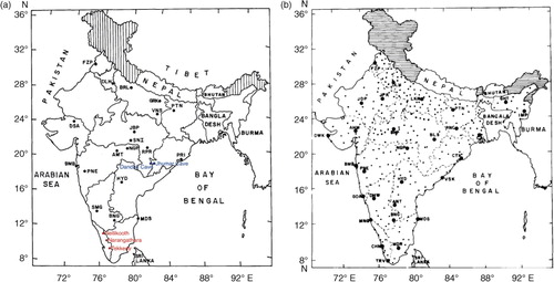
Our period of investigation, 1481–2010, can be divided into two parts: 1844–2010 when instrumental rainfall data from India are available and 1481–1843 when only proxy data are available. Previous studies investigating the relationship between AMV and ISMR in instrumental data have only used the period from 1871 onwards, but rain gauge data from India are available from 1813 (Sontakke et al., 1993). Because the distribution of the stations is quite sparse from 1813 to 1843, only rain gauge data from the year 1844 are studied here, extending the instrumental record by 26 yr. Starting with 10 rain gauge stations in 1844 the number increased progressively to 19 by 1870 (Fig. 2a). Parthasarathy et al. (1994) constructed an ISMR time series from 1871 using rain gauge data from 306 stations well distributed over India (Mooley and Parthasarathy, 1984; Parthasarathy et al., 1987; Fig. 2b), updated annually by the Indian Institute for Tropical Meteorology, Pune, ftp://www.tropmet.res.in/pub/data/rain/iitm-regionrf.txt (see also Parthasarathy et al., 1995). The ISMR time series from Parthasarathy et al. (1994) starting from 1871 forms the basis for the construction of the rainfall series from 1844 to 1870. The criteria for selection of these rain gauge stations are explained by Sontakke et al. (1993). We have combined the ISMR series from Sontakke et al. (1993) and Parthasarathy et al. (1994) to get a continuous rainfall series for the period 1844–2010.

Fig. 2.*  (a) Locations of the 19 selected stations. Mountainous regions (hatched) were not considered for the study. The stations are AMT (Amraoti), BMB (Bombay), BNG (Bangalore), BRL (Bareilly), DSA (Deesa), DLH (Delhi), FZP (Ferozepur), GRK (Gorakhpur), HYD (Hyderabad), JBP (Jabalpur), MDS (Madras), NGP (Nagpur), PTN (Patna), PNE (Pune), PRI (Puri), RPR (Raipur), SMG (Shimoga), SNI (Seoni) and VNS (Varanasi). The locations of the three tree-ring sites used in KTRC are marked in red. The locations of Dandak and Jhumar caves are marked in blue (adapted from Sontakke et al., 1993). (b) Network of 306 rain gauge stations over the area considered excluding hilly area (hatched) (Mooley and Parthasarathy, 1984).

*The geographical boundaries shown in this figure do not necessarily correspond to the political boundaries.

In this study we define dry (wet) years as years with ISMR less (more) than one standard deviation of the long-term mean. Epochs of frequent dry years are defined as a DRY epoch and epochs of infrequent dry years are defined as a WET epoch, as first defined by Joseph (1976). Table 1 shows the dry and wet years identified during the period 1844–2010 making use of instrumental ISMR data. We find that DRY and WET epochs have occurred alternatively since the 1840s. The period 1844–1870 is a DRY epoch with 5 dry years, 1871–1900 is a WET epoch with 3 dry years, 1901–1930 is a DRY epoch with 6 dry years, 1931–1960 is a WET epoch with 2 dry years and 1961–1990 is a DRY epoch with 10 dry years. The period 1991–2020 was expected to be a WET epoch. The first decade of this epoch, 1991–2000, had no dry years; however, since 2001 there have been 5 dry years (2002, 2004, 2014 and 2015), suggesting a possible change in the alternating 30-yr epochal pattern.

Table 1. Dry and wet years of ISMR.

Decade	Decadal mean (mm)	Dry years (<σ of the mean)	Wet years (>σ of the mean)
Period 1844–1870
1844–1850	824.4	1848	–
1851–1860	829.6	1851, 1855, 1860	–
1861–1870	895.0	1864	1861, 1862, 1863, 1867, 1870
Period 1871–2010
1871–1880	849.9	1873, 1877	1874, 1878
1881–1890	881.4		1884
1891–1900	865.5	1899	1892, 1893, 1894
1901–1910	822.4	1901, 1904, 1905	1910
1911–1920	821.3	1911, 1918, 1920	1916, 1917
1921–1930	837.2	–	–
1931–1940	871.3	–	1933
1941–1950	888.8	1941	1942, 1947
1951–1960	871.4	1951	1956, 1959
1961–1970	844.4	1965, 1966, 1968	1961, 1970
1971–1980	840.2	1972, 1974, 1979	1975
1981–1990	831.5	1982, 1985, 1986, 1987	1983, 1988
1991–2000	837.9	–	1994
2001–2010	811.1	2002, 2004, 2009	2007

Standard deviation (σ) of June–September rainfall for the period 1841–1870 = 88.2 mm.

There are several ways to define the AMV index, but all definitions are based on North Atlantic SST anomalies, low-frequency filtered or smoothed to capture multidecadal variability (Kerr, 2000; Enfield et al., 2001). For the instrumental period, we have used the unsmoothed version of the NOAA PSD AMV index starting from 1856, which is the detrended area-weighted average of the Kaplan Extended SST V2 data set (Kaplan et al., 1998) over the North Atlantic (0°N–70°N). We have then averaged the index over the monsoon months (June–September) and smoothed using an 11-yr moving average. As mentioned in Section 1, for the instrumental data, cold and warm phases of the AMV correspond to DRY and WET epochs in the ISMR, respectively (Fig. 1).

3. Available proxy data and selection

Since reliable instrumental data only go back about 150 yr, we need to use proxy reconstructions to study decadal variations in both ISMR and North Atlantic SST before this period. Here we present previously published AMV and ISMR reconstructions with annual resolution, using proxy records from tree rings, speleothems and corals, in order to critically select the data for our analysis.

3.1. ISMR: available proxy data and selection

In the tropics, high precipitation periods favour growth in tree rings, whereas periods of low rainfall inhibit their growth (Pant et al., 1988, 1998; Borgaonkar et al., 1994, 1996; Yadav et al., 1999). Speleothem records can yield similar rainfall estimates as tree rings (Yadava and Ramesh, 1999a, b; Yadava et al., 2004; Yadava and Ramesh, 2005; Sinha et al., 2007). In addition, corals can be used as proxies for the conditions that they live in (Druffel, 1997). By assuming a general relation between ISMR and Indo-Pacific SSTs associated with the El Niño–Southern Oscillation (ENSO) (Rasmusson and Carpenter, 1983; Krishnamurthy and Goswami, 2000), ISMR can be reconstructed using the annual banding in the structure and chemical composition of coral skeletons.

Only six published high-resolution ISMR proxy reconstructions were available to us and are presented here: three based on tree rings, the Kerala tree-ring chronology (KTRC), the statistical model monsoon rainfall (SMMR) and the South Asian summer monsoon index (SASMI); two speleothem records from the Dandak cave and the Jhumar cave; and one coral record from Palmyra Island. All these reconstructions have near-annual resolution and have been studied in relation to ISMR previously (Table 2).

Table 2. Available ISMR proxy reconstructions

Name	Type	Proxy	Period	Region	Resolution	Reference
KTRC	Tree ring	Ring width	1481–2003	Kerala, India	Annual	Borgaonkar et al., 2010
SMMR	Tree ring	Ring width	1602–1960	Global	Annual	1988
SASM	Tree ring	Ring width	896–2000	Asia	Annual	Shi et al., 2014
Dandak Cave	Speleothem	δ ^18O	600–1500	Central India	~Annual	2007
Jhumar Cave	Speleothem	δ ^18O	1075–2008	Central India	~Annual	Sinha et al., 2011
Palmyra coral	Coral	δ ^18O	1635–1702	Equatorial Pacific	Seasonal	Chakraborty et al., 2012

KTRC, Kerala tree-ring chronology; SASM, South Asian summer monsoon; SMMR, statistical model monsoon rainfall.

The Palmyra coral record is short and does not overlap in time with the instrumental record for ISMR, and therefore we cannot evaluate whether this record is able to capture the dry and wet years of ISMR. Both the speleothem records are from the monsoon core region, where local precipitation is strongly correlated with the ISMR index (Gadgil, 2003), and therefore have ideal locations for ISMR reconstructions. The locations of Jhumar and Dandak caves are marked in blue in Fig. 2a. However, the Jhumar cave record, with an average temporal resolution of 1.45 yr, does not capture the dry years in the instrumental record (not shown). Because the Jhumar cave record has lower than annual temporal resolution, it under-samples the dry years and underestimated the interannual variability, and there is no correlation between instrumental ISMR and the Jhumar cave record on these timescales. This record is therefore not appropriate for our analysis as we define dry epochs by the frequency of dry years. The Dandak cave record, as for the Palmyra coral record, is for a period that is not comparable with the instrumental data and hence cannot be evaluated. We therefore chose to continue our analysis with the three tree-ring reconstructions, KTRC, SMMR and SASMI, all with annual resolution.

The KTRC (Borgaonkar et al., 2010) is a tree-ring width chronology of teak (Tectona grandis L.f.) prepared from three sites along the Western Ghats mountains in the state of Kerala for the following overlapping periods: Tekkedy for the period 1785–2003, Narangathara for the period 1742–2003 and Nellikooth for the period 1481–2003. The locations of the three tree-ring sites used in KTRC are marked in red in Fig. 2a. A total of 74 cores from 44 trees from these three sites were subjected to standard dendroclimatic procedures (Stokes and Smiley, 1968; http://ncdc.noaa.gov/paleo/treering.html). Borgaonkar et al. (2010) combined all the tree-ring series to form one single tree-ring width index chronology termed the KTRC. KTRC has been validated using instrumental data and it showed that low tree-ring growth is associated with deficient ISMR since the late 19th century. Before that period, several low tree-ring growth years coincide with El Niño years, which could also be related to deficient ISMR because of the relationship between ISMR and ENSO (Rasmusson and Carpenter, 1983; Krishnamurthy and Goswami, 2000), or with low rainfall years in historical records. Periods with high growth rate may or may not represent wet periods, as excess moisture does not necessarily result in higher tree-ring growth for this data (Borgaonkar et al., 2010). The instrumental ISMR data and KTRC overlap for the period 1844–2003. During the latter half of the 19th century most of the dry years determined from rainfall data are identified in KTRC with an accuracy of ±2 yr. Most of the dry years in the 20th century have been estimated correctly in KTRC, although overestimated during the decade 1941–1950. KTRC is significantly positively correlated with summer monsoon and annual rainfall of Kerala, but has a stronger positive correlation with the instrumental ISMR, suggesting that KTRC captures a larger scale signal than local Kerala rainfall (Borgaonkar et al., 2010).

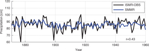
Lough and Fritts (1985) used tree-ring chronologies from both western North America and the Southern Hemisphere to reconstruct the Wright's index (Wright, 1975) of the Southern Oscillation for the period 1600–1961. This is based on the fact that the influence of the Southern Oscillation can be felt on surface climate over a large part of the globe. Pant et al. (1988) used this data to reconstruct the ISMR over the period 1602–1960 (hereinafter SMMR) based on the known relationship between the Southern Oscillation and ISMR. The mean rainfall of ~850 mm as estimated by the SMMR is comparable to that by the rain gauge observations for the period 1871–1960, but the estimated standard deviation is quite low, at 35 mm compared with 81 mm for the rain gauge observations for the same period (Fig. 3). We have estimated the correlation coefficient between instrumental ISMR and SMMR to be 0.43 for this period, statistically significant at a 99% confidence level.

Fig. 3 SMMR (blue) and instrumental ISMR (black) for the period 1871–1960.

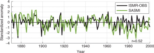
Shi et al. (2014) reconstructed the SASMI for years 896–2000 based on 15 tree-ring chronologies from Asia. A shift in the variability was found in this reconstruction in the mid-17th century (from 1658 AD), and as a result, the occurrence of the extreme monsoon years was investigated by dividing the record into two periods: AD 896–1658 and 1659–2000. We have combined these two periods to get a continuous annual time series of 520 yr for our study period 1481–2000. SASMI values less than or equal to −1.5 represent extreme low years (dry years) and greater than or equal to 1.5 represent extreme high years (wet years) (Shi et al., 2014). Based on these criteria, 27 extreme high and 38 extreme low years were identified for the period 1481–2000. The correlation coefficient between the instrumental ISMR and SASMI during the period 1871–2000 is 0.52, statistically significant at a 99% confidence level (Fig. 4). During this period, the instrumental ISMR recorded 26 dry years (25 wet years) as opposed to 23 extreme low years (12 wet years) estimated by SASMI. SASMI correctly identified 10 out of the 18 dry years (55%) recorded in the instrumental ISMR in the 20th century.

Fig. 4 Standardised anomalies of instrumental ISMR (black) and SASMI (green) for the period 1871–2000.

These three proxy records and the instrumental ISMR data are compared with the India Meteorological Department daily gridded rainfall data (IMDGRD), which has a spatial resolution of 1°×1°, and is available from 1901 (Rajeevan et al., 2005). The correlation between KTRC and the ISMR-index based on the IMDGRD (mean June–September daily rainfall averaged over India) for the 100-yr period (1901–2000) is 0.58, statistically significant at the 99% confidence level, whereas the correlation between SASMI and the IMDGRD ISMR-index for the same period is 0.40, statistically significant at the 99% confidence level. The correlation between SMMR (data available only up to 1960) and the IMDGRD ISMR-index for the 60-yr period (1901–1960) is 0.31, statistically significant at the 95% confidence level.

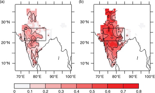
The correlations between KTRC and the daily averaged (June–September) IMDGRD data and between SASMI and IMDGRD data for the period 1901–2000, as well as the correlation between instrumental ISMR and IMDGRD data, are shown in Fig. 5. The box in Fig. 5 indicates Central India (72°E–85°E, 21°N–27°N). Rainfall over Central India has been shown to represent ISMR variation (Gadgil and Joseph, 2003; Rajeevan et al., 2006). KTRC and the instrumental ISMR show a similar spatial pattern with high correlations over the north-west and the Central India box region and low correlations over south peninsular India and north-eastern regions. SASMI also has higher correlations over the Central India box region along with the northern and western parts of India. The correlations between SMMR and IMDGRD for the 60-yr overlapping period and the correlations between instrumental ISMR and IMDGRD for the same period are shown in Fig. 6. The areal extent of the high positive correlations of SMMR with IMDGRD is similar to that of KTRC with IMDGRD but slightly weaker. The positive correlations are again found to be high over the Central India box region. The correlation analysis has shown that all three tree-ring-based proxy records are able to capture the spatial and temporal rainfall pattern over India.

Fig. 5 The correlation between IMDGRD data and (a) KTRC, (b) SASMI and (c) instrumental ISMR for the period 1901–2000. For KTRC, the correlation is calculated by representing dry years by 1 and non-dry years by 0. Contours show correlations significant at 90% confidence level. The black box indicates the Central India box (72°E–85°E, 21°N–27°N).

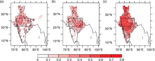
Fig. 6 The correlation between IMDGRD data and (a) SMMR and (b) instrumental ISMR for the period 1901–1960. Contours show correlations significant at 90% confidence level. The black box indicates the Central India box (72°E–85°E, 21°N–27°N).

3.2. AMV: available proxy data and selection

There are presently three available annual-resolution multi-proxy AMV reconstructions: the reconstructions from Gray et al. (2004), Mann et al. (2009) and Svendsen et al. (2014) (Table 3). The record from Gray et al. (2004) is based on tree-ring records from around the North Atlantic and spans the years 1567–1990. Mann et al. (2009) used a global proxy data set comprising thousands of tree ring, ice core, coral, sediment and other proxy records spanning the ocean and land regions of both hemispheres over the past 1500 yr to reconstruct surface temperature changes on a global scale. In this study, we have used the AMV data reconstructed by Mann et al. (2009) for the period that overlaps with the ISMR reconstructions, years 1481–2006. The record from Svendsen et al. (2014) is reconstructed using five marine-based proxy records from massive-growing tropical coral colonies from the North Atlantic Ocean and covers the years 1781–1986. These three proxy reconstructions of AMV have been validated earlier, and they compare well in the instrumental period (Svendsen et al., 2014); however, discrepancies between the records are present before this period. At the moment, we do not know which of these reconstructions are more reliable, and more high-resolution proxy reconstructions are needed to assess these discrepancies (Kilbourne et al., 2014; Svendsen et al., 2014).

Table 3. Available AMV proxy reconstructions used in this study

Name	Type	Period	Reference
Gray-AMV	Tree ring	1567–1990	Gray et al., 2004
Mann-AMV	Multi-proxy	500–2006	Mann et al., 2009
Svendsen-AMV	Coral	1781–1986	Svendsen et al., 2014

AMV, Atlantic multidecadal variability.

4. Evaluation of decadal variability in ISMR prior to the instrumental period

Decadal variability in North Atlantic SST anomalies before the instrumental period has been evaluated in earlier studies (Gray et al., 2004; Mann et al., 2009; Svendsen et al., 2014). In this section, we evaluate the decadal variability of ISMR in the three proxy reconstructions chosen in Section 3: KTRC, SMMR and SASMI.

4.1. Decadal variability in KTRC

In KTRC, we find, as in Borgaonkar et al. (2010), that there are several lengthy low-growth periods, indicating decadal variability in ISMR. We have grouped the KTRC data of Borgaonkar et al. (2010) into seven temporal clusters of frequent dry years with a total of 86 dry years (Table 4 and Fig. 7a). The total duration of these DRY epochs (A1–G1) is 282 yr, with an average frequency of one dry year in about 3 yr. The periods between the DRY epochs, which may be called WET epochs, had only six dry years (1581, 1594, 1600, 1724, 1735 and 1778) in a total duration of 228 yr, with a frequency of 1 dry year in 38 yr. These frequencies compare well with the frequencies of dry years in DRY and WET epochs in the instrumental period. The time difference in years between the middle points of the successive DRY epochs is 55, 123, 86, 70, 73 and 57 yr, which may be taken as the period of the decadal variation. The period is in the range of 55–86 yr, except for one long 123-yr period, comparable to the decadal variability of both AMV and ISMR during the recent century and a half with instrumental measurements. Because KTRC only gives us an estimate of the timing of dry years, we quantify the wet and dry years by constructing a rainfall time series based on KTRC, where dry years are represented by 1 and non-dry years by 0. An 11-yr moving average of this rainfall series, divided by 11 to get the probability of a dry year, is given in Fig. 7a. The seven DRY epochs described earlier are clearly seen in the figure. In some 11-yr periods in these clusters, the probability of a dry year reaches 40–50%. The timing of the dry clusters in KTRC is comparable to the observed DRY epochs (Fig. 7a). The number of observed dry years during the period 1844–1877 is more or less matched by the KTRC data. However, the number of dry years in the earlier half of the 20th century (1900–1930) is overestimated by KTRC (dry cluster F1), whereas the number of dry years in the latter half of the 20th century (from 1970s) is underestimated (dry cluster G1).

Fig. 7 ISMR reconstruction made with (a) KTRC (red), (b) SMMR (blue) and (c) SASMI (green), where dry years are represented by 1 and non-dry years are represented by 0, and then an 11-yr moving average has been performed. The bars show the number of dry years per 11-yr period divided by 11 (probability of a dry year). The 11-yr moving average of instrumental ISMR with dry years represented by 1 and non-dry years by 0 is shown in black in all panels.

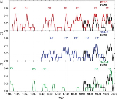
Table 4. Epochs of frequent dry years from 1481 to 2003 derived from KTRC

Dry epoch	Dry years
(A1) 1484–1515	1484, 1486, 1491, 1492,1508,1510,1512,1514,1515
(B1) 1539–1571	1539, 1540, 1541, 1552,1564,1565,1569,1570,1571
(C1) 1652–1703	1652, 1656, 1663, 1665, 1666, 1676, 1680, 1681, 1691, 1693, 1694, 1696, 1700, 1703
(D1) 1760–1767	1760, 1761, 1763, 1765, 1767
(E1) 1791–1877	1791, 1794, 1802, 1803, 1811, 1812, 1814, 1818, 1821, 1824, 1829, 1832, 1833, 1837, 1838, 1844, 1853, 1865, 1868, 1873, 1877
(F1) 1896–1918	1896, 1899, 1901, 1904,1905,1908,1911,1914,1915,1918
(G1) 1941–1987	1941, 1944, 1945, 1949, 1951, 1954, 1959, 1965, 1966, 1967, 1968, 1972, 1979, 1982, 1987

4.2. Decadal variability in SMMR

In the SMMR, as for the instrumental ISMR, we define those years with rainfall less than one standard deviation lower than the long-term mean as dry years. Table 5 gives a complete list of the dry years and indicates clusters of frequent dry years in the SMMR reconstruction for the period 1602–1960. Many of the dry and wet years in instrumental ISMR are correctly identified by SMMR (Table 5 and Figs. 3 and 7b). The alternating 30-yr DRY and WET epochs seen in the instrumental ISMR data are also discernible in SMMR. During the 90-yr period (1871–1960) that overlaps the instrumental period, 15 dry years were identified in the SMMR as opposed to 11 in the instrumental record, with a hit rate of 73% (11 out of 15), indicating that SMMR is effective in identifying dry rainfall years. The last cluster of dry years from 1897 to 1930 (epoch E2) coincides well with the DRY epoch in the instrumental ISMR from 1899 to 1920 (Fig. 7b and Table 1). The cluster of dry years in SMMR from 1676 to 1720 (epoch A2) covers a major part of DRY epoch C1 in KTRC, 1743–1776 (epoch B2) includes DRY epoch D1 and the periods 1790–1811 (epoch C2) and 1863–1876 (D2) are part of DRY epoch E1 in KTRC. The five DRY epochs given by SMMR have a total duration of 149 yr and a total number of 41 dry years, with an average frequency of 1 dry year per 3.6 yr. This compares well with the frequency of dry years in DRY epochs of ISMR in the instrumental rainfall period.

Table 5. Epochs of frequent dry years from 1602 to 1960 derived from SMMR

Dry epoch	Dry years
(A2) 1676–1720	1676, 1679, 1682, 1688, 1700, 1702, 1705, 1717, 1720
(B2) 1743–1776	1743, 1746, 1747, 1754, 1755, 1758, 1760, 1768, 1769, 1775, 1776
(C2) 1790–1811	1790, 1792, 1799, 1807, 1808, 1811
(D2) 1863–1876	1863, 1864, 1868, 1876
(E2) 1897–1930	1897, 1899, 1902, 1904, 1911, 1912, 1913, 1914, 1918, 1925, 1930

4.3. Decadal variability in SASMI

For SASMI, we have taken the low extreme years and high extreme years as defined by Shi et al. (2014) as the dry and wet years, respectively. Table 6 lists the dry years and frequent clusters of dry years identified by SASMI for the period 1481–2000. Instrumental ISMR and SASMI overlap for the period 1844–2000, and SASMI has correctly identified 12 out of the 26 dry years during this period. In Fig. 7c, it can be seen that SASMI also exhibits multidecadal variability consistently during the period 1481–2000. The DRY epoch E3 during the instrumental period coincides with the KTRC DRY epoch G1. The long DRY epoch D3 in the early 20th century covers the DRY epoch E2 in SMMR and F1 in KTRC, though the number of dry years identified by SASMI in this epoch is considerably lower than that identified by the other two tree-ring-based reconstructions. In general, the number of dry years identified by SASMI during the pre-instrumental period is low. The DRY epoch C3 which contains 3 dry years in a 10-yr period forms a part of epoch A2 in SMMR and epoch C1 in KTRC. The epoch A3 during the late 15th century is part of epoch A1 in KTRC. The total duration of DRY epochs in SASMI is 89 yr, including a total of 30 dry years with an average frequency of 1 dry year per 3 yr.

Table 6. Epochs of frequent dry years from 1481 to 2000 derived from reconstructed SASMI

Dry epoch	Dry years
(A3) 1481–1495	1481, 1482, 1484, 1492, 1495
(B3) 1600–1603	1600, 1602, 1603
(C3) 1651–1663	1651, 1653, 1663
(D3) 1902–1931	1902, 1905, 1914, 1915, 1920, 1926, 1931
(E3) 1965–1992	1965, 1966, 1968, 1976, 1979, 1980, 1982, 1983, 1986, 1987, 1991, 1992

5. Relation between ISMR and AMV

As seen in previous studies, the 30-yr DRY and WET epochs in the instrumental ISMR time series coincide with the cold and warm phases in observed AMV (Fig. 1). Previous studies have also shown that multidecadal variability in North Atlantic SSTs has persistence prior to the instrumental records, and the section above suggests that multidecadal variability has persistence in the ISMR as well. Here we compare the three selected ISMR proxy reconstructions (SMMR, SASMI and KTRC) with the three available AMV reconstructions (Gray-AMV, Mann-AMV and Svendsen-AMV) to investigate the stability of the observed AMV-ISMR relationship. We have used the negative of the KTRC record because dry years were defined as 1 and other years were defined as 0. Such a quantitative comparison of annual-resolution ISMR proxy reconstructions has never been published, and in light of recent modelling studies on the AMV-ISMR link, a comparison with available AMV reconstructions is overdue. In the following analysis, we have used an 11-yr moving average filter on all the time series. We have also tested our results with other more advanced filters and found that the results are similar. The published AMV index from Mann et al. (2009) is already low-pass filtered, and this data is therefore not additionally smoothed for our analysis.

The instrumental and proxy reconstructed AMV and ISMR indices have a common overlapping period of 131 yr (1856–1986), except for SMMR that only covers the years up to 1960. The linear correlation coefficients between all these indices are estimated for this common period and for the entire length of the two indices being compared (Table 7). For the common period, there are statistically significant correlations between all the AMV proxy data with the observed AMV, with the Gray-AMV having the highest correlation of 0.83. All the three proxy reconstructions of ISMR have a positive correlation with the instrumental ISMR index although for KTRC the correlation is not significant. Because KTRC is made up of 1s and 0s, the autocovariance of this smoothed record will be high. This leads to a smaller number of effective degrees of freedom, and significant correlations with this filtered record will be difficult to obtain.

Table 7. Linear correlation coefficients between AMV and ISMR indices normalised and smoothed with an 11-yr moving average for the period 1856–1986.

Linear correlation	Gray-AMV	Mann-AMV	Svendsen-AMV	Observed ISMR	KTRC	SMMR^#	SASMI
Observed AMV	0.83^a(0.83^a, 1856–1990)	0.55^c (0.54^c,1856–2006)	0.52^c (0.52^c,1856–1986)	0.64^a (0.43^c,1856–2010)	0.35 (0.33,1844–2000)	0.52^c (0.52^c,1856–1960)	0.66^a (0.61^a,1856–2000)
Gray- AMV		0.78^a (0.50^a,1567–1990)	0.42^c (0.33,1781–1986)	0.55^b (0.51^b,1844–1990)	0.26 (0.06, 1567–1990)	0.27 (−0.03,1602–1960)	0.40 (0.05,1567–1990)
Mann-AMV			0.39 (0.47^c,1781–1986)	0.30 (0.03,1844–2006)	0.07 (−0.07,1491–2000)	0.22 (−0.19,1602–1960)	0.11 (−0.12,1481–2000)
Svendsen-AMV				0.49^c (0.48^b,1844–1986)	0.16 (0.10,1781–1986)	0.83^a (0.46^b,1781–1960)	0.59^b (0.45^b,1781–1986)
Observed ISMR					0.42 (0.32,1844–2000)	0.56^c (0.45^c,1844–1960)	0.57^a (0.54^a,1844–2000)
KTRC						0.57^b (0.41^b,1602–1960)	0.29 (0.11,1491–2000)
SMMR							0.82^a (0.25^c,1602–1960)

The values in parenthesis give the correlation during the entire record length and the years covered. ^# Linear correlation coefficient is calculated for the common period 1856–1960. ^a,b,cValues appearing with the superscripts a, b and c indicate significance at a confidence level of 99, 95 and 90%, respectively, for the effective degrees of freedom. AMV, Atlantic multidecadal variability; ISMR, Indian summer monsoon rainfall; KTRC, Kerala tree ring chronology; SASMI, South Asian summer monsoon index; SMMR, statistical model monsoon rainfall.

The correlation between the observed AMV and instrumental ISMR for the whole period (1854–2010) is, as earlier mentioned, 0.43; however, this reaches to 0.64 when we only take into account the shorter overlapping common period 1856–1986. The correlation seems sensitive to end points, but the observed AMV and ISMR have diverged since the end of the 1990s (Fig. 1). The observed AMV is positively correlated with all the three ISMR proxy series, where the correlation with SASMI is the highest, and the correlation with KTRC is the weakest. However, when we calculate the correlations between the AMV and ISMR proxy reconstructions for the entire length of the records, the correlation between AMV and ISMR breaks down (Table 7). There is no significant correlation between the AMV and ISMR proxy records, except between Svendsen-AMV and SMMR, which has the shortest overlapping period. The three ISMR proxy records (KTRC, SASMI and SMMR) even show negative correlation with Mann-AMV for their whole overlapping periods. Although the proxy reconstructions for both AMV and ISMR have positive correlations with the observed records, the positive AMV-ISMR correlation does not persist throughout the time period studied here back to 1481.

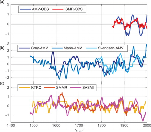
The filtered time series of the various observed and proxy data of ISMR and AMV over the entire period of their availability back until 1481 are shown in Fig. 8. The instrumental ISMR and observed AMV during the recent one and a half centuries are shown in Fig. 8a. It is clear that during the 20th century ISMR and AMV are more or less in phase, except for at the very end of the century. We can also see that the DRY ISMR epoch identified in the earlier instrumental records from 1844 to 1860 corresponds to a cold period in the reconstructed AMV indices. The AMV proxy data are in good agreement until the mid-18th century (Fig. 8b), but they deviate during the decades prior to this, which is consistent with the correlations in Table 7. The ISMR proxy reconstructions KTRC, SASMI and SMMR are somewhat in agreement with each other during the time period available for comparison (1602–1960), except during the 18th century when all the three data differ in phase over a number of decades (Fig. 8c), which is consistent with the results shown in Fig. 7. In the 16th century when only KTRC and SASMI are available for comparison, both of them are in disagreement during majority of the decades but are in phase during the end of the century. It should be kept in mind that KTRC only gives a qualitative measure of the dry years and does not distinguish between excess and normal rainfall years, possibly leading to some of these phasing differences. The discrepancies between the proxy reconstructions emphasise the importance of using several reconstructions when comparing proxies. Similarly, Kilbourne et al. (2014) investigated the AMV using several proxy reconstructions (including Gray-AMV and Mann-AMV used in this study) and found no consensus during the pre-instrumental era.

Fig. 8 (a) Instrumental AMV and ISMR, (b) proxy reconstructed AMV (Gray-AMV, Mann-AMV and Svendsen-AMV) and (c) proxy reconstructed ISMR (KTRC, SASMI and SMMR). All the time series data are normalised and smoothed using an 11-yr moving average, except Mann-AMV which is only available as a filtered product.

6. Discussion and conclusions

Decadal variability of ISMR for the recent five centuries has been studied here using instrumental rain gauge data and available high-resolution proxy reconstructions. From these sources, we have documented the dry years. From the period of instrumental data (1844–2010), we found that this period had alternate 30-yr epochs of frequent dry years and infrequent dry years. The epochs 1844–1870, 1900–1930 and 1961–1990 had frequent dry years, with an average of 1 dry in every 3 yr, and the decadal mean ISMR was below the long-time average. The 30-yr epochs 1871–1900 and 1931–1960 had very few dry years and the decadal mean ISMR was above the long-time average. The period 1484–1843 had several epochs of frequent dry years (DRY epochs), with about 1 dry year in 3 yr on average, and the decadal variability had a period of 55–86 yr. Thus, during the entire period (1484–2010), a prominent multidecadal signal is present in the ISMR.

The link between the AMV and ISMR during the period 1481–2010 was analysed by comparing these ISMR records with instrumental data and available proxy reconstructions of AMV. For the period when instrumental data were available for comparison, we see that during the WET (DRY) epochs of ISMR the North Atlantic Ocean had warmer (colder) than normal SSTs. However, our analyses showed that the observed positive correlation between the AMV and ISMR during the last century and half cannot be seen before 1750, although multidecadal variability with a period of 60–80 yr is seen in the proxy reconstructions of both ISMR and AMV. For instance, during the period 1600–1650, all the ISMR records are in positive phases and both the longer AMV records are in negative phases. Here, the records agree on a negative correlation in contrast to that seen during the time period of instrumental data. We also notice that the observed AMV-ISMR link has weakened in the recent decade, suggesting that the positive correlation between these two regions is not stable. There has been a consistent weakening trend in the ISMR in the second half of the 20th century, while AMV has been in a positive phase during the last two decades. This weakening trend in the ISMR has been related to, for instance, an increase in aerosol emissions (Ramanathan et al., 2005; Bollasina et al., 2011). Similarly, external forcing, such as variations in solar irradiance as well as both anthropogenic and volcanic aerosols, has been suggested as a possible modulator for the Atlantic multidecadal oscillation (Otterå et al., 2010; Booth et al., 2012). Hence, we can speculate that external forcing could have played a role in the correlation between multidecadal variability of ISMR and Atlantic SSTs. For instance, during the 100 yr period from around 1650 to 1750, the variability in both the AMV and ISMR proxy data sets (Fig. 8b–c) as well as the correlation between them is low. This could be related to the low volcanic activity in the same period (Otterå et al., 2010).

We have validated the data sets used, and as concluded in Section 3 we found that the three ISMR reconstructions we have used (KTRC, SASMI and SMMR) were the most ideal for this analysis. However, there are drawbacks in these data sets also and proxy reconstructions have uncertainties related to sampling and dating error. For instance, the KTRC data set is based on tree rings from only one region in India, the state of Kerala. Although the correlation between ISMR and rainfall in the state of Kerala is statistically significant, the record is likely to include regional rainfall variability. However, this record seems to capture a majority of the instrumental ISMR dry years, and Borgaonkar et al. (2010) state that KTRC has a stronger correlation with ISMR than local summer rainfall in Kerala. SMMR is based on a reconstruction of the Southern Oscillation and takes advantage of the observed relationship between ENSO and ISMR. Even though the relationship between ISMR and ENSO has been strong in the instrumental period, there are several studies indicating that this relationship has broken down since the 1990s (Krishna Kumar et al., 1999). The SMMR reconstruction depends on a stable ENSO–ISMR relationship, which might not be realistic. In addition, the SMMR data are reconstructed using tree-ring chronologies from both western North America and Southern Hemisphere. Hence, the signal found in SMMR might not be completely independent of AMV, and this could possibly explain the correlation between SMMR and the proxy reconstructions of AMV. SASMI makes use of tree-ring chronologies from 15 different locations in Asia and is able to identify many of the dry years in the instrumental ISMR and about 69% of the historical famine events recorded in India in the last millennium (Shi et al., 2014). However, the number of dry years recorded prior to the instrumental era is considerably lower than that recorded by both KTRC and SMMR. This could be related to the fact that most of the tree-ring chronologies come from sites outside the ISMR domain, or that the SASMI uses a stricter criterion for defining dry years. In addition to the uncertainties in the ISMR proxy reconstructions, the AMV reconstructions also deviate prior to the year 1750, except during the period 1600–1650 when both the longer records are in negative phases. Because of inconsistencies in available proxy records for both AMV and ISM, more high-quality reconstructions are needed to assess the link between AMV and ISMR before the 1800s. The results presented here indicate that the AMV-ISM link might not be as clear as previous studies have suggested, and the weakening correlation in the recent decade further supports these results.

Previous studies have identified a robust relationship between North Atlantic SST and the Asian monsoon on millennial timescales using low-resolution proxy data (Gupta et al., 2003; Jung et al., 2004). The results found here are not in disagreement with this, as our focus has been on shorter timescales of variability using annual-resolution proxy data. SST anomalies in the Atlantic approximated for millennial timescale variations including periods of major climate shifts are larger than those characterising the AMV during the past 500 yr and could therefore also have larger impacts.

To summarise, we find that the observed correlation between AMV and ISMR monsoon rainfall extends back to the 18th century. However, none of the records show consistent positive correlations prior to that period, and all the records diverge before the 1800s, except for a short period in the first half of the 1600s. Uncertainties in the proxy reconstructions contribute to the insignificant correlations we find between AMV and ISMR before the 18th century, and the results imply that better quality data are required to be conclusive, and caution should be exercised when using single proxy reconstructions for comparing with records from other regions as well as with model simulations. However, the weakening of the AMV-ISMR link observed in the last decade suggests that other physical mechanisms for driving multidecadal variability in the ISMR could also be important, for example, the SST gradient between the tropics and Northern mid-latitudes suggested by Joseph et al. (2013) and the impact of aerosol forcing on both AMV (Otterå et al., 2010; Booth et al., 2012) and ISMR (Bollasina et al., 2011; Ramanathan et al., 2005).

7. Acknowledgements

We thank the authors of the proxy reconstructions used in this study for making their reconstructions available to the community, especially Dr G. B. Pant and co-authors for supplying the rainfall data derived from global tree rings using a statistical method. We also thank Dr H. P. Borgaonkar for useful discussions regarding the Kerala tree ring series derived by Borgaonkar et al. (2010). We are grateful to Prof. Noel Keenlyside and the anonymous reviewers for helping us to improve the manuscript. This work was performed as part of Project INDIA-CLIM (#216554) funded by the Research Council of Norway, with Prof. Ola M. Johannessen as the project leader. One of the authors, G. Bindu, was funded by the EU-INDO-MARECLIM project coordinated by Nansen Environmental Research Centre India (NERCI).

References

- Bollasina M. A. , Ming Y. , Ramaswamy V . Anthropogenic aerosols and the weakening of the South Asian summer monsoon. Science. 2011; 334(6055): 502–505.
- Booth B. B. , Dunstone N. J. , Halloran P. R. , Andrews T. , Bellouin N . Aerosols implicated as a prime driver of twentieth-century North Atlantic climate variability. Nature. 2012; 484(7393): 228–232.
- Borgaonkar H. P. , Pant G. B. , Rupa Kumar K . Dendroclimatic reconstruction of summer precipitation at Srinagar Kashmir India since the late18th Century. Holocene. 1994; 4: 299–306.
- Borgaonkar H. P. , Pant G. B. , Rupa Kumar K . Ring-width variations in Cedrusdeodara and its climate response over the Western Himalaya. Int. J. Climatol. 1996; 16: 1409–1422.
- Borgaonkar H., Sikder A., Ram S., Pant G. El Nino and related monsoon drought signals in 523-year-long ring width records of teak (Tectona grandis L.f.) trees from south India. Palaeogeogr. Palaeoclimatol. Palaeoecol. 2010; 285(1–2): 74–84. DOI: http://dx.doi.org/10.1016/j.palaeo.2009.10.026.
- Burns S. J. , Fleitmann D. , Matter A. , Kramers J. , Al-Subbary A. A . Indian Ocean climate and an absolute chronology over Dansgaard/Oeschger events 9 to 13. Science. 2003; 288: 847–850.
- Chakraborty S. , Goswami B. N. , Dutta K . Pacific coral oxygen isotope and the tropospheric temperature gradient over the Asian monsoon region: a tool to reconstruct past Indian summer monsoon rainfall. J. Quaternary Sci. 2012; 27(3): 269–278.
- Druffel E. R. M . Geochemistry of corals: proxies of past ocean chemistry, ocean circulation, and climate. Proc. Natl. Acad. Sci. USA. 1997; 94(16): 8354–8361.
- Enfield D. B. , Mestas-Nunez A. M. , Trimble P. J . The Atlantic multidecadal oscillation and its relationship to rainfall and river flows in the continental U.S. Geophys. Res. Lett. 2001; 28: 2077–2080.
- Feng S., Hu Q. Regulation of Tibetan Plateau heating on variation of Indian summer monsoon in the last two millennia. Geophys. Res. Lett. 2005; 32: L02702. DOI: http://dx.doi.org/10.1029/2004GL021246.
- Feng S., Hu Q. How the North Atlantic Multidecadal Oscillation may have influenced the Indian summer monsoon during the past two millennia. Geophys. Res. Lett. 2008; 35: L01707. DOI: http://dx.doi.org/10.1029/2007GL032484.
- Gadgil S . The Indian Monsoon and its variability. Annu. Rev. Earth Planet. Sci. 2003; 31: 429–67.
- Gadgil S. , Joseph P. V . On breaks of the Indian monsoon. Proc. Indian Acad. Sci. (Earth Planet. Sci.). 2003; 112(4): 529–558.
- Goswami B. N., Madhusoodanan M. S., Neema C. P., Sengupta D. A physical mechanism for North Atlantic SST influence on the Indian summer monsoon. Geophys. Res. Lett. 2006; 33: L02706. DOI: http://dx.doi.org/10.1029/2005GL024803.
- Gray S. T., Graumlich L. J., Betancourt J. L., Pederson G. T. A tree-ring based reconstruction of the Atlantic Multidecadal Oscillation since 1567 A.D. Geophys. Res. Lett. 2004; 31: L12205. DOI: http://dx.doi.org/10.1029/2004GL019932.
- Gupta A. K., Anderson D. M., Overpeck J. T. Abrupt changes in the Asian southwest monsoon during the Holocene and their links to the North Atlantic Ocean. Nature. 2003; 421: 354–357. DOI: http://dx.doi.org/10.1038/nature01340.
- Joseph P. V . Climate change in monsoon and cyclones. 1976. Proceedings of IITM symposium on Monsoons. 1976; Pune. 378–387. September 8–10.
- Joseph P. V., Bindu G., Nair A., Wilson S. S. Variability of summer monsoon rainfall in India on inter-annual and decadal time scales. Atmos. Ocean. Sci. Lett. 2013; 6: 398–403. DOI: http://dx.doi.org/10.3878/j.issn.1674-2834.13.0044.
- Jung S. J. A. , Davies G. R. , Ganssen G. M. , Kroon K . Synchronous Holocene sea surface temperature and rainfall variations in the Asian monsoon system. Q. Sci. Rev. 2004; 23: 2207–2218.
- Kaplan A. , Cane M. A. , Kushnir Y. , Clement A. C. , Blumenthal M. B. , co-authors . Analysis of global sea surface temperature 1856–1991. J. Geophys. Res. 1998; 103: 18567–18589.
- Kerr R. A . A North Atlantic climate pacemaker for the centuries. Science. 2000; 288(5473): 1984–1986.
- Kilbourne K. H. , Alexander M. A. , Nye J. A . A low latitude paleoclimate perspective on Atlantic multidecadal variability. J. Mar. Syst. 2014; 133: 4–13.
- Krishna Kumar K. , Rajagopalan B. , Cane M. A . On the weakening relationship between the Indian monsoon and ENSO. Science. 1999; 284: 2156–2159.
- Krishnamurthy V. , Goswami B. N . ENSO–Monsoon relationship on interdecadal time scales. J. Clim. 2000; 13: 579–595.
- Li S., Perlwitz J., Quan X., Hoerling M. P. Modelling the influence of North Atlantic multidecadal warmth on the Indian summer rainfall. Geophys. Res. Lett. 2008; 35: L05804. DOI: http://dx.doi.org/10.1029/2007GL032901.
- Lough J. M. , Fritts H. C . The Southern Oscillation and Tree Rings: 1600–1961. J. Clim. Appl. Meteorol. 1985; 24: 952–966.
- Luo F., Li S., Furevik T. The connection between the Atlantic Multidecadal Oscillation and the Indian Summer Monsoon in Bergen Climate Model Version 2.0. J. Geophys. Res. 2011; 116: D19117. DOI: http://dx.doi.org/10.1029/2011JD015848.
- Mann M. E., Zhang Z., Rutherford S., Bradley R., Hughes M. K., co-authors. Global signatures and dynamical origins of the Little Ice Age and Medieval Climate Anomaly. Science. 2009; 326: 1256–1260. DOI: http://dx.doi.org/10.1126/science.1177303.
- Mooley D. A. , Parthasarathy B . Fluctuations in all India summer monsoon rainfall during 1871–1978. Clim. Change. 1984; 6: 287–301.
- Otterå O. H. , Bentsen M. , Drange H. , Suo L . External forcing as a metronome for Atlantic multidecadal variability. Nat. Geosci. 2010; 3(10): 688–694.
- Overpeck J., Anderson D., Trumbore S., Prell W. The southwest Indian Monsoon over the last 18000 years. Clim. Dynam. 1996; 12: 213–225. DOI: http://dx.doi.org/10.1007/BF00211619.
- Pant G. B. , Borgaonkar H. P. , Rupa Kumar K . Climatic signals from tree-rings; a dendroclimatic investigation of Himalayan spruce (Piceasmithiana). Himalayan Geol. 1998; 19(2): 65–73.
- Pant G. B. , Rupa Kumar K. , Borgaonkar H. P . Statistical models of climate reconstruction using Tree-ring data. Proc. Indian Natl. Sci. Acad. 1988; 50A, 1988: 354–364.
- Parthasarathy B. , Munot A. A. , Kothawale D. R . All India monthly and seasonal rainfall series: 1871–1993. Theor. Appl. Climatol. 1994; 49: 217–224.
- Parthasarathy B. , Munot A. A. , Kothawale D. R . Monthly and seasonal rainfall series for all-India homogeneous regions and meteorological subdivisions: 1871–1994. 1995; Indian Institute of Tropical Meteorology, Pune, Research Report No. RR 065.
- Parthasarathy B. , Sontakke N. A. , Munot A. A. , Kothawale D. R . Droughts/floods in the summer monsoon season over different meteorological subdivisions of India for the period 1871–1984. J. Climatol. 1987; 7: 57–70.
- Rajeevan M. , Bhate J. , Kale J. D. , Lal B . Development of a high resolution daily gridded rainfall data for the Indian region. 2005; IMD Met Monograph No, India Meteorological Department, Pune, India: Climatology 22/2005. 27.
- Rajeevan M. , Bhate J. , Kale J. D. , Lal B . High resolution daily gridded rainfall data for the Indian region: Analysis of break and active monsoon spells. Curr. Sci. 2006; 91(3): 296–306.
- Ramanathan V. , Chung C. , Kim D. , Bettge T. , Buja L. , co-authors . Atmospheric brown clouds: Impacts on South Asian climate and hydrological cycle. Proc. Natl. Acad. Sci. USA. 2005; 102(15): 5326–5333.
- Rasmusson E. M. , Carpenter T. H . The relationship between eastern equatorial Pacific sea surface temperature and rainfall over India and Sri Lanka. Mon. Weather Rev. 1983; 111: 517–528.
- Shi F., Li J., Wilson R.J. A tree-ring reconstruction of the South Asian summer monsoon index over the past millennium. Sci. Rep. 2014; 4: 6739. DOI: http://dx.doi.org/10.1038/srep06739.
- Sinha A., Berkelhammer M., Stott L., Mudelsee M., Cheng H., co-authors. The leading mode of Indian Summer Monsoon precipitation variability during the last millennium. Geophys. Res. Lett. 2011; 38: L15703. DOI: http://dx.doi.org/10.1029/2011GL047713.
- Sinha A., Cannariato K. G., Scott L. D., Cheng H., Lawrence Edwards R., co-authors. A 900-year (600 to 1500 AD) record of the Indian summer monsoon precipitation from the core monsoon zone of India. Geophys. Res. Lett. 2007; 34: L16707. DOI: http://dx.doi.org/10.1029/2007GL030431.
- Sontakke N. A. , Pant G. B. , Singh N . Construction of all-India summer monsoon rainfall series for the period 1844–1991. J. Clim. 1993; 6: 1807–1811.
- Stokes M. A. , Smiley T. L . An Introduction to Tree-ring Dating. 1968; The University of Chicago Press, Chicago, IL. 73.
- Sutton R. T. , Hodson D. L. R . Atlantic Ocean forcing of North American and European summer climate. Science. 2005; 309: 115–118.
- Svendsen L., Hetzinger S. Z., Keenlyside N., Gao Y. Marine based multiproxy reconstruction of Atlantic multidecadal variability. Geophys. Res. Lett. 2014; 41: 1295–1300. DOI: http://dx.doi.org/10.1002/2013GL059076a.
- Ting M., Kushnir Y., Seager R., Li C. Robust features of Atlantic multi-decadal variability and its climate impacts. Geophys. Res. Lett. 2011; 38: L17705. DOI: http://dx.doi.org/10.1029/2011GL048712.
- Wright P. B . An index of the southern oscillation. 1975; Rep. No. CRU-RP4 Climatic Research Unit. University of East Anglia, Norwich, UK. 22.
- Yadav R. R. , Park W. K. , Bhattacharya A . Spring temperature fluctuations in the western Himalayan region as reconstructed from tree-rings; AD1390–1987. Holocene. 1999; 9: 85–90.
- Yadava M. G. , Ramesh R . Paleomonsoon record of the last 3400 years from speleothems of tropical India. Gondwana Geol. Mag. 1999a; 4: 141–156.
- Yadava M. G. , Ramesh R . Speleothems – useful proxies for past monsoon rainfall. J. Sci. Ind. Res. 1999b; 58: 339–348.
- Yadava M. G. , Ramesh R . Monsoon reconstruction from radiocarbon dated tropical Indian speleothems. Holocene. 2005; 15(1): 48–59.
- Yadava M. G. , Ramesh R. , Pant G. B . Past monsoon rainfall variations in peninsular India recorded in a 331-year-old speleothem. Holocene. 2004; 14(4): 517–524. ISSN 0959-6836.
- Zhang R., Delworth T. L. Impact of Atlantic multidecadal oscillations on India/Sahel rainfall and Atlantic hurricanes. Geophys. Res. Lett. 2006; 33: L17712. DOI: http://dx.doi.org/10.1029/2006GL026267.