Regularised empirical orthogonal functions^†

† The review process was handled by Chief Editor Peter Lundberg.

Abstract

Empirical orthogonal functions, extensively used in weather/climate research, suffer serious geometric drawbacks such as orthogonality in space and time and mixing. The present paper presents a different version, the regularised (or smooth) empirical orthogonal function (EOF) method, by including a regularisation constraint, which originates from the field of regression/correlation of continuous variables. The method includes an extra unknown, the smoothing parameter, and solves a generalised eigenvalue problem and can overcome, therefore, some shortcomings of EOFs. For example, the geometrical constraints satisfied by conventional EOFs are relaxed. In addition, the method can help alleviate the mixing drawback. It can also be used in combination with other methods, which are based on downscaling or dimensionality reduction. The method has been applied to sea level pressure and sea surface temperature and yields an optimal value of the smoothing parameter. The method shows, in particular, that the leading sea level pressure pattern, with substantially larger explained variance compared to its EOF counterpart, has a pronounced Arctic Oscillation compared to the mixed North Atlantic Oscillation/Arctic Oscillation pattern of the leading EOF. The analysis of the remaining leading patterns and the application to sea surface temperature field and trend EOFs are also discussed.

• EOFs
• Regularised EOFs
• Generalised eigenvalue problem
• North Atlantic Oscillation
• Arctic Oscillation

1. Introduction

Empirical orthogonal function (EOF) analysis is one of the earliest and most widely used method in the atmospheric science (Obukhov, 1947, 1960; Lorenz, 1956). The EOF analysis method can be used in different ways and can be adopted to various contexts (Jolliffe, 2002); that is, the EOFs are multipurpose. They can be used, for example, to identify modes of variability and propagating structures and permit dimensionality reduction. They can be applied in weather forecasting, statistical modelling, climate model validation, etc.; see, for example, the reviews of Hannachi et al. (2007) and Monahan et al. (2009).

The original context of EOFs (Obukhov, 1947; Fukuoka, 1951; Lorenz, 1956) was to achieve a decomposition of a continuous space–time field X(t,s), such as sea level pressure (SLP), where t and s denote, respectively, time and spatial location, as1

using an optimal set of basic functions of space a _k () and expansion functions of time c _k (). The expansion [eq. (1)] is also known as Karhunen Loève expansion (Loève, 1978). In practice, we are given a (centred) data matrix X=(x _ij ), i=1, … n, and j=1,… d, where n is the sample size and d is the number of grid points or degrees of freedom. Then, the EOF method finds a linear combination of the variables, that is, a set of weights u=(u ₁, …, u _d ) ^T , such that the time series Xu has maximum variance. The EOFs are then obtained by solving the following eigenvalue problem:2

where and represents the covariance matrix of the gridded data field X.

EOFs are known to have a number of drawbacks resulting from the orthogonality in space and time, namely orthogonality of the EOF patterns and uncorrelatedness of the associated time series or principal components (PCs); see, for example, Jolliffe (2002), Hannachi (2007) and Monahan et al. (2009). Some alleviation methods have been proposed in the literature to relax the above-mentioned geometric constraints. Most of these methods are based on some sort of EOF rotation (Richman, 1986; Hannachi et al., 2007, 2009), but they all share a common feature, namely the lack of physicality as they are all geometrical in essence. Other methods have been proposed based, for example, on simplicity (Hannachi et al., 2006), optimal interpolation (Hannachi, 2008), optimal persistence (DelSole, 2001) or teleconnection (van Den Dool et al., 2000). These methods, however, are not directly linked to EOF analysis. Tipping and Bishop (1999) proposed probabilistic PC analysis. The method is reminiscent of factor analysis (e.g. Jolliffe, 2002). Though appealing, as it is based on a probabilistic model, the method maximises the likelihood via an iterative expectation–maximisation algorithm and therefore misses the benefit of the exact singular value decomposition algorithm.

Most weather/climate variables, for example, spatial fields, are of continuous nature. Conventional methods of multivariate data analysis deal mostly with observations at discrete steps, such as gridded data. Conventional EOF method is an example. Note, however, that the original context of EOFs was to obtain a decomposition of continuous fields as pointed out above [see eq. (1)]

The simulation of weather and climate has advanced to a point where scientists are now running global forecast models at very high resolutions. Climate models are lagging a bit behind regarding resolution but are not very far from their forecast analogues. The paradox, however, is that for practical purposes, in general, using gridded data fields with very high resolution can be a handicap particularly in the application of statistical and statistical–dynamical models in weather forecasting, downscaling, climate impact studies, etc. This has led to the development of methods to reduce the dimension of the state vector based, for example, on random projection (Seitola et al., 2014, 2015), which can reduce the problem size down to 1% of the original size. Although this method reduces the problem size of eq. (2) and thus the computational load, the aforementioned drawbacks, such as mixing, are not alleviated.

The main objective of this paper is twofold: (i) it attempts to address some of the drawbacks of the EOFs mentioned above regarding the geometric constraints, and (ii) addresses the issue of spatial continuity. In brief, the method considers finding the EOFs of a continuous field. Dealing with continuous fields, however, can lead to a kind of indeterminacy, which can be overcome by introducing some sort of regularisation (or smoothing). First, the regularisation procedure transforms the eigenvalue problem [eq. (1)] into a generalised eigenvalue problem, leading to the regularised or smooth EOFs, and consequently may overcome the issue of space–time orthogonality and related drawbacks such as mixing. Second, EOF regularisation provides a remedy to the drawback of downscaling the resolution. The paper can also be used for didactive purposes in addition to the epistemological value of the method. The author was not aware of a similar work in the literature except the paper of Wang and Huang (2016), which was brought to the author's attention by the reviewers. The objective of Wang and Huang (2016), however, is different from that of the present paper in that it aims at reducing the noise in the modes of variability particularly when the sample size is smaller than the number of variables, while conserving the spatial orthogonality property. In the remainder of the paper, the terms ‘regularised’ and ‘smooth’ EOFs will be used interchangeably.

The manuscript is organised as follows. Section 2 provides a background on the root of the problem, which emerges from functional canonical correlation analysis (CCA) and its indeterminacy. Section 3 discusses the smooth EOF method. An application to the sea surface temperature (SST) and SLP fields in addition to trend EOFs (TEOFs) is presented in Section 4, and a summary and discussion are given in the last section. Readers who are not interested in the technical details can skip to Section 3.4, which provides a brief summary of the method.

2. Functional and smooth CCA

2.1. Functional non-smooth CCA and indeterminacy

Continuous fields require in principle special attention in many cases. Before we discuss the problem of ‘regularised’ or ‘smooth’ EOFs of continuous fields it is instructive and also didactive to go to the root of the problem. The problem originates, in fact, in the field of regression and correlation analysis between two continuous variables or fields. For instance, in CCA and maximum covariance analysis (MCA) one seeks linear combinations of two fields that have maximum correlation or covariance, respectively. Let us assume, in the start, that we are given a sample of two continuous curves x _k (s) and y _k (s), k=1, … n. The variable s is now a continuous parameter varying in some finite interval I and n is again the sample size. For simplicity, we assume that the curves have been centred to have zero-mean, that is, , for all values of s within the above interval. This is like removing the ensemble mean of each field from each curve. Note that ′s′ here plays the role of variables in the discrete case and the index k refers to observation or realisation. Linear combinations of x _k (s) now involve ‘continuous’ weights, for example, function a(s), and take the form of an integral, that is,3

In a similar manner to the standard discrete case, the objective of functional CCA is to find functions (or weights) a(s) and b(s) such that the cross-correlation between the linear combinations <a, x _k > and <b, y _k > is maximised. If we designate by S _xy () the covariance function between x and y, that is, S _xy (r,s)=E[x(r)y(s)], then the optimisation problem, applied to the population yields:4

subject to the condition:5

Note that eq. (5) is required to make the problem bounded, with a unique solution. As for conventional CCA, the optimisation problem [eqs. (4) and (5)] yields the eigenvalue problem:6

which can be written as a single generalised (integral) eigenvalue problem in matrix form.

In practice, we do not know the population covariance function which has to be estimated from the available sample. Now when the above result is applied to the sample curves, it turns out that there are always functions a(s) and b(s) that guarantee perfect correlation between the corresponding linear combinations <a, x _k > and <b, y _k >, k=1, … n. Furthermore, Leurgans et al. (1993) show that any linear combination of x _k can be made perfectly correlated with the corresponding linear combination of y _k , k=1, … n. This points to a conceptual problem, known as the indeterminacy problem, in estimating functional CCA from a finite sample using eqs. (4) and (5). This problem is overcome by introducing some sort of smoothing in the estimation as is shown next.

2.2. Smooth or regularised CCA/MCA

The above indeterminacy problem in continuous CCA is normally solved through some sort of ‘regularisation’ or ‘smoothing’. The regularisation procedure in CCA is similar to the idea of spline smoothing (Tikhonov, 1963; Morozov, 1984) used as a way to smoothly interpolate discrete data by means of piece-wise polynomials (Schoenberg, 1964; Wahba, 2000). To achieve this, the constraints [eq. (5)] are penalised by a smoothing condition taking the following form:7

where α is referred to as the smoothing parameter and is also unknown; see also Ramsay and Silverman (2006). Equation (4) subject to the smoothing constraint [eq. (7)] constitutes the basic problem of the regularised (or smooth) CCA.

To solve the optimisation problem [eq. (4)] subject to the smoothing constraints [eq. (7)], a few assumptions on the regularity of the functions involved are required. To ease the flow of the text, one considers the notations; for the natural scalar product between the weight functions a() and b(), and as the ‘weighted’ scalar product between a() and b(). The functions involved, as well as their mth derivatives, m=1, … 4, are supposed to be square integrable over the interval I. To simplify the equations, it is also assumed that the functions and their first four derivatives have periodic boundary conditions; that is, if I=[τ ₀,τ ₁], then , m=1, … 4. These conditions make the second-order differential operator D ²(), that is, D ² a=d ² a/ds ², defined over the set of functions presented above over the interval I self adjoint with respect to the scalar product <,>₁ and yields, through integration by parts, a simpler form of the constraints.

With these conditions, we have the following result:

Theorem

The solution to the problem [eqs. (4) and (7)], that is:

where and similarly for D^mb, is necessarily given by the solution to the following integro-differential eigenvalue problem:8

The same procedure can also be applied to the MCA to yield smooth MCA. In fact, smooth MCA is similar to smooth CCA except that the constraint conditions [eq. (7)] are replaced by:9

The optimisation problem [eq. (4)], subject to the normalisation constraint [eq. (9)], yields the following system of integro-differential equations:10

2.3. Application of smooth MCA to continuous fields

We now suppose that we have two continuous spatial fields F(x,t _k ) and G(y,t _k ), observed at times t _k , k=1, … n, where x and y represent continuous spatial locations. We also assume that the coordinates x and y vary in two spatial domains and , respectively. The covariance function between the (zero-mean) fields F and G at x and y is given by:11

The objective is then to identify (continuous) spatial patterns u(x) and v(y) maximising the integrated covariance, that is,12

subject to the smoothing constraints13

where ∇² u=Δu and represents the Laplacian of u and similarly for v. In the Cartesian plane, for example, where x=(x ₁,x ₂), the Laplacian of u(x) is . The situation is exactly similar to eqs. (4) and (10) except that now one is dealing with spatial fields, and one gets the following integro-differential system:14

3. Functional and regularised EOFs

3.1. Basic problem formulation

Functional EOF analysis is concerned with EOF analysis applied to data which consist of curves or surfaces. In atmospheric science, for example, the observations consist of spatio-temporal fields that represent a discrete sampling of continuous variables, such as pressure or temperature at a set of finite grid points. Functional and smooth EOFs correspond to smooth MCA, as given by eq. (10), when the left and right fields are identical. Let us first look at the case of curves. We suppose that we are given a sample of n curves that constitute the coordinates of a vector curve x(s)=(x ₁(s), …, x _n (s)) ^T , with zero-mean, that is, for all values of s. The covariance function is given by:15

where r and s are in the domain of the definition of the curves. The problem then is to find smooth functions (EOFs) a(s), for all s in I, maximising subject to a normalisation constraint condition of the type <a, a>₁+ α <D ² a,D ² a>₁ −1=0. The solution to this problem is then given by the following integro-differential equation:16

The case of non-smooth EOFs, corresponding to α=0, is simply referred to as functional EOFs. One way to obtain functional non-smooth EOFs is to decompose the function a(.) using a set of basis functions and obtain a linear system for the weights; see, for example, Jolliffe and Cadima (2016).

3.2. Case of spatial fields

Here we suppose that we observe a sample of zero-mean space–time field F(x,t _k ) at times t _k , k=1, …, n and x represents a spatial position. In a similar manner to eq. (11), the covariance function of the field is given by:17

We denote by Ω the spatial domain, which can be the entire globe or a limited geographical region. The objective of smooth EOFs is to find the regularised EOFs of the covariance matrix [eq. (17)]. Such an EOF is a continuous pattern, u(x), solution to the optimisation problem:18

This yields a similar integro-differential equation to eq. (16), namely;19

Here we suppose that α is given, and we focus more on the application to observed fields. The choice of the smoothing parameter α will be discussed later. The case of functional non-smooth (α=0) EOFs can be explored in terms of basis functions such as radial basis functions, but we do not discuss this here and we focus on the smooth EOF solution discussed below.

3.3. Numerical solution of smooth EOFs

Let us define the sampled space–time field through a (centred) data matrix X=(x ₁, …, x _d ), where x _k =(x _1k , …, x _nk ) ^T is the time series of the field at the kth grid point, and the associated sample covariance matrix S. We remind the reader here that the integral [eq. (19)] is an area integral, that is,20

In spherical coordinates dΩ=R ²cos(ϕ)dϕdλ, where R is the Earth's radius, ϕ and λ are the latitudinal and longitudinal coordinates, respectively. The integral expression and the differential operator can be numerically discretised. The pattern u=(u ₁, …, u _d ) ^T satisfying the discretised version of eq. (19) or (20) is approximated by the solution to the following generalised eigenvalue problem:21

In eq. (21), D ⁴ is the square of the (discretised) Laplacian operator ∇², which is self adjoint (see, e.g., Roach, 1970).

In spherical coordinates, the Laplacian is:22

The discretised Laplacian yields a matrix whose elements are functions of the latitudinal coordinates, and can be computed explicitly. The discretised version of the Laplacian ∇² u of the function u(ϕ,λ), based on a simple finite difference scheme in spherical coordinates at grid point (ϕ _k ,λ _l ) reads:

for k=1, …, p, and l=1, …, q and where u _k,l =u(ϕ _k ,λ _l ), with ϕ _k , k=1, …, p, and λ _l , l=1, …, q, being the discretised latitude and longitude coordinates, respectively. Note that here q and p represent, respectively, the resolutions in the zonal and meridional directions, so the total number of grid points is d=pq. In eq. (21), the matrix is given by the following Hadamard (or element-wise) product:24

where Φ= φ 1, with φ being the pq×1 column vector containing q replicates of the vector (cosϕ ₁,…cosϕ _p ) ^T , that is, φ =(cosϕ ₁, … cosϕ _p , … cosϕ ₁, … cosϕ _p ) ^T and 1 is the 1×pq vector of ones. Note that eq. (24) simply represents the area weighting of the covariance matrix usually used to take into account the converging meridiens at the poles. Note that in eq. (23) the discretisation in the meridional and zonal directions is assumed to be uniform. We point out here that in spectral methods, for example, the latitudes are on a Gaussian grid where δϕ _k =ϕ _k+1 − ϕ _k is not uniform. This can be easily taken into account in eq. (23).

Since eq. (20) involves a differential operator the solution to the problem requires boundary conditions, which are used to compute the matrix D ⁴ in eq. (21). The discussion here is limited to three basic types of boundary conditions, which can cover most of the remaining conditions. We consider first the case of hemispheric fields for which one can take ϕ ₀=π/2, ϕ _k+1=ϕ _k − δϕ, and λ _q =λ ₁ (periodicity condition). One can also take u _0,l =0, and u _p+1,l =u _p,l , l=1, …, q, plus the periodic boundary condition u _k,q+1=u _k,1. Let us define , that is, the vector u represents the spatial pattern measured at the grid points (ϕ _k ,λ _l ), k=1, …, p, and l=1, …, q, where . After a little algebra one gets:25

where C and A are p×p matrices given, respectively, by26

and27

where , , and c _k =(δλcosϕ _k )⁻². Note that A is tridiagonal, and the operator D ² is symmetric and near-bloc tridiagonal because of the upper right and lower left non-zero elements. The eigenvalue problem [eq. (21)] yields28

which is a generalised eigenvalue problem when the smoothing parameter α≠0 is given. In the above equation, I _pq is the pq×pq identity matrix.

In the above system, we have assumed that u _0l =0, for l=1, … q, meaning that the pattern is zero at the pole. This condition may be reasonable perhaps for the wind field but not for other variables such as pressure or temperature. The second case considers the more practical boundary condition for hemispheric fields by considering for example:

This constitutes, in fact, a very good condition as the meridiens converge poleward in spherical coordinates. In this case, we obtain a similar system matrix to that of eq. (25), that is:29

where is similar to , see eqs. (25) and (27), in which A=(a _ij ) is replaced by B=(b _ij ) where and b _ij =a _ij for all other i and j.

In the third case, we now assume that the field is not periodic in the zonal direction where we investigate instead a limited rectangular region on the sphere. In this case, we can assume:

in the zonal direction whereas in the meridional direction the same condition of case 2 still holds, that is, u _0l =u _1l and u _p+1,l =u _pl , for l=1, … q. In this case, and recalling the matrix B given in eq. (29), eq. (25) yields:30

which goes into eq. (21). Note that in this case, the matrix of eq. (30) is bloc tridiagonal.

3.4. Summary of the method

To recapitulate what has been done above, we assume that we are given a sample of gridded dataset F(x,t _k ), observed at times t _k , k=1, … n. One first computes the covariance matrix S, eq. (17), and its weighted expression , eq. (24). Next the matrices , and , given, respectively, by eqs. (25), (29) and (30) are computed. For a given regularisation parameter α, the regularised EOFs are obtained as the solution to the generalised eigenvalue problem [eq. (28)] using either , or . The use of , or depends on the boundary conditions, or in other words, the type of the domain of the observed field. For example, for global or hemispheric (periodic) fields the matrix is used if the field vanishes at the pole, otherwise is used. If the field is regional instead, that is, observed over a localised domain then is used.

3.5. Choice of the smoothing parameter

There is no universal way to obtain the smoothing parameter α. The parameter can be obtained, for example, from experience. Another method is to use a cross-validation (cv) procedure based on what is known as leave-one-out approach. For a given α, the total misfit is computed by removing, each time, one observation from the sample, and computing the residuals using a given number of smooth EOFs. The cv is then obtained by computing the variance of the residuals. The optimal value of α is the one that provides the smallest variance. Here, however, the cv is not a good measure and that is because the EOFs are the only patterns that minimise the residual variance. Here, an alternative way is used based on the Lagrangian of eq. (18), that is,31

and the objective is to analyse versus α and identify whether there is an optimal value of α maximising in eq. (31).

In theory, near the optimum the term between brackets, in the right hand side of eq. (31), should be small and the Lagrangian should be the dominant term. In practice, however, this may not be the case and care must be taken when computing the Lagrangian, such as avoiding getting too close to the pole to avoid singularity of the matrix A, eq. (27), and choosing the right scaling. For example, in eq. (28), the Earth's radius is fixed to 65 so that and R ⁴ nearly balance each other (particularly in the extratropics), and the remaining part of R is absorbed by α.

4. Application

The method has been applied to two datasets; the observed SST and the SLP fields. The SLP data1 represent monthly fields obtained from the National Center for Environmental Prediction/National Center for Atmospheric Research (NCEP/NCAR). The data are on a 2.5° latitude–longitude resolution grid and span the period Jan 1948–Dec 2015. The SST data come from the Hadley Centre Sea Ice and Sea Surface Temperature2 (HadISST). The data are a combination of globally complete monthly fields of SST and sea ice on a 1°×1° latitude–longitude grid from 1870 to date (Rayner et al., 2003). The analysis is restricted to the period Jan 1870–Dec 2014.

4.1. SLP analysis

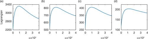
The SLP anomalies are computed by removing the climatological monthly seasonal cycle. The analysis focuses primarily on the extratropical Northern Hemisphere (NH) north of 17.5° N, and comments on the equatorial region are given later. For the NH, the discussion is primarily on the winter, December–February, months, but the analysis is extended to include all months for comparison. The SLP anomalies are downgraded by selecting four different resolutions, namely 2.5°×2.5°, 5°×5°, 5°×10° and 10°×10° latitude–longitude grids. To analyse the relevance of the smoothing parameter, the Lagrangian , eq. (31), was computed for the leading smooth EOF as a function of this parameter, but using the few leading smooth EOFs does not change significantly the results. Figure 1 shows versus α for the four downgraded resolutions. Two main features can be read from the figure. First, the curves have a maximum showing the existence of an optimal value for the smoothing parameter. This shows clearly that (conventional) EOFs do not necessarily provide an optimal value of the (regularised) Lagrangian. Second, the optimal value increases as the resolution decreases. This is an equally important result reflecting the importance of smoothing for sparse gridded data.

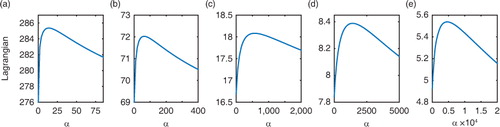
Fig. 1 Lagrangian versus the smoothing parameter α calculated using eq. (31), based on the leading smooth EOF of the extratropical NH SLP anomalies for 2.5°×2.5° (a), 5°×5° (b), 5°×10° (c) and 10°×10° (d) latitude–longitude grid.

The eigenvalues of the regularised problem, based on the optimal value of α, of the order 1.16×10⁴ (see Fig. 1d) for the lowest resolution, that is, 10° grid, are shown in Fig. 2 along with the corresponding values for the conventional (α=0) EOFs. Note also that regularised EOFs are quite robust to small changes of the smoothing parameter α. The eigenvalues are scaled by the total variance of the SLP anomalies and multiplied by 100, and therefore they represent the explained variance of the associated EOFs, and approximately3 the ‘explained’ variance of the smooth EOFs. Of particular interest is the (scaled) eigenvalue (or explained variance) of the leading smooth EOF. This variance is about one and a half times larger than the value of the corresponding leading EOF (Fig. 2). The leading four smooth EOFs are discussed here and compared to the corresponding EOFs. Figure 3 shows the leading two conventional and smooth EOFs calculated based on the lowest resolution, that is, 10° latitude–longitude grid, and using the corresponding optimal smoothing parameter α (Fig. 1d).

Fig. 2 Eigenvalues µ of the generalised eigenvalue problem [eq. (21)] for the winter SLP anomalies over the Northern Hemisphere for the smoothed problem (filled circle) and the non-smoothed (α=0) problem (open circle). The eigenvalues are scaled by the total variance of the SLP anomalies and transformed to a percentage, so, for example, the spectra given by the open circles provide the percentage of explained variance of the EOFs.

Fig. 3 Leading two EOFs (a, c) and regularised EOFs (b, d) of the Northern Hemisphere SLP anomalies based on the 10°×10° latitude–longitude grid. The smoothing is based on the optimal value of the Lagrangian (Fig. 1d).

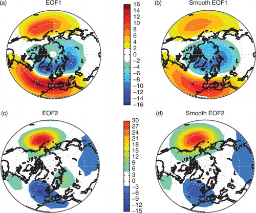
The leading EOF (Fig. 3a) is accepted (in the literature) as a general representation of the Arctic Oscillation (AO), although the structure of the pattern is seen to contain a strong component of the North Atlantic Oscillation (NAO), for more discussion on the NAO/AO dichotomy the reader is referred to Ambaum et al. (2001). The point here is that EOF1 is strongly asymmetric with more NAO structure over the North Atlantic region than the supposedly nearly zonally symmetric structure of the AO. The smoothing shows indeed that the leading pattern (Fig. 3b) reflects the quasi-symmetric AO pattern, which may explain the larger explained variance compared to that of EOF1 (Fig. 2). Note that as the smoothing parameter increases beyond the optimal value the leading smooth EOF (not shown) becomes more zonally symmetric particularly over the polar region.

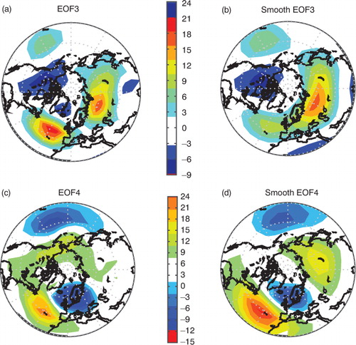
The second EOF (Fig. 3c) and smooth EOF (Fig. 3d) patterns are quite similar and represent the North Pacific pattern. The smooth EOF3 (Fig. 4b) is dominated by two main centres of action sitting, respectively, over Eurasia and North America, unlike the EOF3 (Fig. 4a) with three main centres of action with the strongest sitting over the North Atlantic. The smooth EOF4 (Fig. 4d) shows clearly the wavy structure of the Scandinavian pattern emanating from the North Atlantic and reaching the North Pacific as a Rossby wave train following great circles (Hoskins and Karoly, 1981; Hoskins and Ambrizzi, 1993). The Scandinavian pattern in EOF4 (Fig. 4c), however, is not as clear as that of Fig. 4d.

Fig. 4 As in Fig. 3 but for the third and fourth EOFs (a, c) and smooth EOFs (b, d) patterns.

Another interesting feature of the spectrum of Fig. 2, which is not investigated further here, is the existence of equal eigenvalues such as the case of the (4,5) or (8,9) pairs. These pairs are most likely associated with propagating structures. The associated smooth EOFs (not shown) are in fact phase shifted with respect to each other. The associated time series are highly correlated, but without high lagged correlation. The shortness of the times series does not allow a genuine investigation of this issue. It is possible to identify a propagating signal using high-frequency data such as daily time series. This suggests in fact that smooth EOFs can be used in connection with extended EOFs (Hannachi et al., 2007) to identify better propagating signals from gridded data.

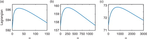
Smooth EOFs have also been examined using monthly SLP anomalies over the equatorial region 17.5 °S–17.5 °N. The Lagrangian for this case is shown in Fig. 5 for three different resolutions, showing the same features discussed previously. The leading smooth EOF (not shown) reflects the southern oscillation signal and is neater than the leading EOF (not shown), but the difference, however, is not substantial. It is worth pointing here that as the latitudes are close to zero the non-zero elements of the smoothing matrix in eqs. (27) and (30) are approximately uniform.

Fig. 5 As in Fig. 1 but for the SLP anomalies over the tropical region for 2.5° (a), 5° (b) and 7.5° (c) latitude–longitude grid.

One notes here that the patterns of the smooth EOFs of the downscaled resolutions (e.g. Figs. 3 and 4) might not look as smooth as the name indicates. This is simply due to the plotting routine. One might argue, on the other hand, that it is perhaps easier to simply take the conventional EOFs and then apply any spatial smoothing. Although this is possible, it remains, however, ad hoc and entirely artificial. The proposed method indeed overcomes this as it consistently formulates the problem in its proper framework. It also provides objectively the value of the smoothing parameter in additions to the explained variances.

4.2. SST analysis

The SST anomalies are computed by removing the monthly seasonal cycle climatology. The domain considered here is limited meridionally to the region 45.5°S–45.5°N. Five different downgraded resolutions are considered, namely 2°, 4°, 8°, 12°, and 16° latitude–longitude grids, respectively. Figure 6 shows the Lagrangian versus the smoothing parameter α for the various downscaled resolutions. The figure shows similar features as those of Fig. 1.

Fig. 6 As in Fig. 1 but for the SST anomalies based on the 2° (a), 4° (b), 8° (c), 12° (d) and 16° (e) latitude–longitude grids.

The eigenvalues of the generalised eigenvalue problem (Fig. 7) show, like the EOF spectra, that the leading two patterns are well separated from the rest. The eigenvalues associated with the EOFs are slightly larger than those obtained from the regularised problem. To compare the EOF and smooth EOF patterns, the focus is shifted mainly on the leading two patterns. Figure 8 shows the leading two EOFs (Fig. 8a and c) and associated smooth EOFs (Fig. 8b and d) for the lowest resolution (16°), using the optimal value of the smoothing parameter α, of the order 0.43×10⁴ (Fig. 6e). Perhaps one of the main differences is the absence, in the regularised patterns, of small scale features as those near the Californian coast and east of the Japanese coast near the Kuroshio current region (Fig. 8a). This is partly because the regularised EOFs tend to focus more on larger scales, and partly because they reduce the drawback related to mixing observed in (conventional) EOFs. The second peak in EOF1 located in the central Pacific (Fig. 8a) vanishes from the smooth EOF1 (Fig. 8b). The double peaks on the equator in EOF1 has also been smoothed out yielding one single maximum in the El-Niño pattern of the smooth EOF1 in the eastern equatorial Pacific.

Fig. 7 As in Fig. 2 but for the SST anomalies at 16° latitude–longitude resolution grid.

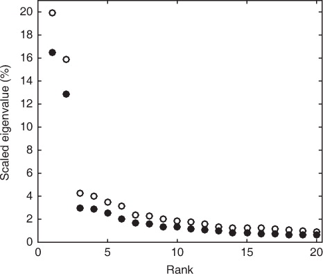
Fig. 8 Leading two EOFs (a, c) and smooth EOFs (b, d) of the SST anomalies using the 16°×16° latitude–longitude grid. The smoothing is based on the optimal value of the Lagrangian (Fig. 6e).

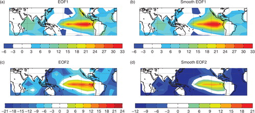
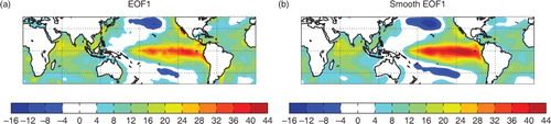
The second EOF (Fig. 8c) shows again a double peak near the central and eastern equatorial Pacific. This has again been smoothed out in smooth EOF2 (Fig. 8d). A similar behaviour is obtained with higher resolution fields. The double peaks structure in EOF2 has been also smoothed out in the smooth EOF2. Figure 9 shows the leading EOF and the corresponding smooth EOF for the 2° latitude–longitude resolution of the SST anomalies. Again the multiple peaks in the tropical Pacific and other small scale structures are either removed or substantially reduced in the smooth pattern. For larger smoothing parameters, for a given resolution, the signal in the eastern Pacific detaches from the coast (not shown).

Fig. 9 Leading EOF (a) and smooth EOF (b) of the SST anomalies using the 2°×2° latitude–longitude grid and the optimal smoothing parameter (Fig. 6a).

4.3. Application in connection to TEOFs

Smooth EOFs can also be applied in combination with TEOFs. TEOFs, for example, Hannachi (2007) and Barbosa and Andersen (2009), are obtained by finding trend patterns from gridded data. They are based on ranks data, and therefore the method of smooth EOFs can be applied naturally here to obtain regularised TEOFs. As a matter of fact the same SLP data used in Hannachi (2007) is considered here and the TEOFs, combined with the smoothing procedure, are computed. TEOFs are based on the EOFs of the inverse of ranks of the data, and the presence of trends is identified by a small number of leading eigenvalues well separated from a ‘noise’ floor (Hannachi, 2007). The TEOFs are then obtained as the eigenvectors of the covariance, or correlation matrix (of the inverse ranks) associated with those eigenvalues. Note here that the covariance and correlation matrices are similar since we are dealing with ranks. Since they are based on inverse ranks, the TEOFs are not in the physical space. To obtain the trend patterns (in the physical space), the data anomalies are first projected onto the TEOFs, and the obtained time series are then regressed back onto the data anomalies.

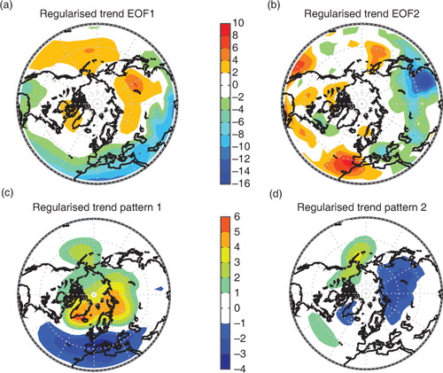
The data used by Hannachi (2007) consist of a 2.5°×2.5° latitude–longitude NCEP/NCAR SLP anomalies for the period 1948–2000, and two trend patterns were identified, namely the NAO pattern and the Siberian High (Panagiotopoulos et al., 2005). The data resolution is reduced to 5°×5° grid and the spectrum of the inverse ranks covariance matrix computed using smooth (with the optimal smoothing parameter α=60) and non-smooth cases. Figure 10 shows the spectrum for the non-smooth (Fig. 10a) and smooth or regularised (Fig. 10b) cases along with the 95% confidence interval following the rule-of-thumb of North et al. (1982). Figure 10a shows that reducing the resolution has led to the second trend being missing, compared to the case of the original data (Hannachi, 2007). When the TEOF method is applied with smoothing the second eigenvalue is raised off the spectrum floor (Fig. 10b) and the second trend pattern regained (Fig. 10b). The regularised trend PCs associated with the leading two eigenvalues (Fig. 10b) are shown in Fig. 10c and d, more discussion on the nature of the trend PCs can be found in Hannachi (2007). Figure 11a and b shows the leading two TEOFs. The third TEOF (not shown) has no structure and is consistent with (trend) noise. As it is pointed out above, the TEOFs are not in the physical space, and the trend patterns in the physical space are obtained via double projection. The associated trend patterns are shown in Fig. 11c and d, and represent, respectively, the NAO pattern (Fig. 11c) and the Siberian High (Fig. 11d), as in Hannachi (2007).

Fig. 10 Eigenspectrum, given in terms of percentage of explained variance, of the covariance (or correlation) matrix of the inverse ranks of the SLP anomalies with a reduced resolution of 5°×5° grid for the non-regularised (a) and regularised (b) cases, along with the regularised first (c) and second (d) trend PCs associated with the leading two eigenvalues shown in (b). The optimal smoothing parameter, α=60, is used in (b).

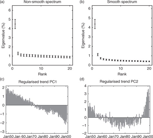
Fig. 11 The leading two regularised trend EOFs (a, b) of the SLP anomalies, corresponding to the leading two eigenvalues of Fig. 10b, and the associated trend patterns (c, d) obtained by projecting the SLP anomalies onto the trend EOFs and then regressing back onto the same anomalies. Contour interval in (c, d) is 1 hPa.

5. Summary and discussion

Smooth or regularised EOF method is presented in this paper. Unlike conventional EOFs, which are obtained by solving a simple eigenvalue problem, regularised EOFs are obtained by solving a generalised eigenvalue problem. The problem is formulated via penalising the constraints using a regularisation term involving the integral of the Laplacian of the field. Being a solution of a generalised eigenvalue problem, the regularised EOFs relax the severe geometric constraints, for example, orthogonality in space and time and mixing, characterising them.

The regularised EOFs involve an extra unknown, the smoothing parameter, which has to be chosen before solving the generalised eigenvalue problem. The Lagrangian of the optimisation problem is used here to estimate the smoothing parameter as the cross-validation procedure is not appropriate for this particular problem. It is worth pointing out that the method is not about artificially smoothing the EOFs as one might think, but formulates the problem in its proper framework in a consistent manner.

The method has been applied to monthly SLP and SST data. Various resolutions are used through downgrading the original data. The analysis of the Lagrangian versus the smoothing parameter reveals the existence of an optimum of this parameter reflecting the significance of the regularisation method. The analysis also shows that the optimal smoothing parameter increases with decreasing resolution reflecting the worthiness of the method for sparse data.

The application to the northern hemispheric SLP anomalies isolates the leading smooth EOF with an explained variance substantially larger than that of the leading EOF. Compared to the mixed NAO/AO pattern of EOF1, the leading smooth EOF clearly shows the AO pattern. Among the other teleconnections obtained, the fourth smooth EOF shows a more consistent Scandinavian pattern with its propagating structure, compared to the less pronounced pattern of EOF4. The application to the equatorial belt shows that the leading smooth EOFs compare with the corresponding EOFs, but remain smoother.

The application to the SST anomalies, over the region 45 °S–45 °N, shows comparable eigenvalue spectra between the EOFs and the smooth EOFs. Small scales have been smoothed out with regularised EOFs, notably the local structures around the Californian coast and the Kuroshio current, reducing hence the mixing drawback. In addition, the El-Niño signal of the smooth EOF1 emerges with one single peak in the eastern equatorial Pacific compared to the double peak in EOF1. Similar smoothed features are also obtained with the second smooth EOF compared to the corresponding EOF.

Regularised EOFs have also been applied in connection with TEOFs, which are based on the eigenvalue decomposition of the covariance matrix of the inverse ranks of the data (Hannachi, 2007). The method was applied to the same data used by Hannachi (2007) after downgrading the resolution to 5°×5°. With this new resolution, the TEOF method was unable to capture the second trend mode, that is, the Siberian High (Panagiotopoulos et al., 2005). However, when the regularisation procedure was applied, the second trend pattern was regained.

Regarded as a perturbation of the EOF method, the smooth EOF method provides a ‘natural’ alternative to, and provides a way towards reducing some of the drawbacks of EOFs. Furthermore, due to increasing computer power and improving climate models, scientists are now starting to produce very high resolution weather/climate data on a large scale including forecasts and reanalyses. This can pause a handicap to the application of, for example, statistical or dynamical–statistical models. Random projection has been proposed by Seitola et al. (2014, 2015) to reduce problem size, but does not alleviate the drawbacks of the EOF method. Another simple alternative is to reduce the number of grid points and then compute the EOFs. In this case, regularised EOFs provide the appropriate tool that may be used in combination with the previous method to ‘regain’ the ‘continuity’ of the weather/climate fields. The orthogonality property is also relaxed with the smooth EOF method. However, since the method is considered as a small perturbation of the conventional method, the patterns are close to being, but not exactly, orthogonal.

Regularised EOF method was shown to be able to separate the AO from the NAO, and also rose the eigenvalue of the leading regularised EOF compared to that of the conventional EOF. In case of SST field, however, although the percentage of explained variance of the leading EOF and that of the regularised EOF are comparable (with a slightly larger value for EOF1), the latter contained less mixed features such as those related to the Kuroshio current or small secondary peaks. The reason for not rising the eigenvalue of the regularised EOF1, compared to that of EOF1, is not entirely obvious, but could possibly be due to the fact that El-Niño is the dominant mode of climate variability in the tropical ocean and does not tend to be mixed with other major modes of variability.

6. Acknowledgements

The author would like to thank two anonymous reviewers for their constructive comments that helped improve the manuscript.

Notes

1 www.esrl.noaa.gov/psd/data/gridded/data.ncep.reanalysis.surface.html

† The review process was handled by Chief Editor Peter Lundberg.

2 www.metoffice.gov.uk/hadobs/hadisst/

3 This is because the smoothed problem can be regarded as a perturbation of the EOF problem, and the matrix in the right hand side of eqs. (28–30) is approximately symmetrical, making the eigenvalues look like variances of the (‘smoothed’) data matrix.

References

- Ambaum M. H. P. , Hoskins B. J. , Stephenson D. B . Arctic oscillation or North Atlantic oscillation?. J. Clim. 2001; 14: 3495–3507.
- Barbosa S. M. , Andersen O. B . Trend patterns in global sea surface temperature. Int. J. Climatol. 2009; 29: 2049–2055.
- DelSole T . Optimally persistent patterns in time-varying fields. J. Atmos. Sci. 2001; 58: 1341–1356.
- Fukuoka A . A Study of 10-Day Forecast (A Synthetic Report), Vol. XXII. 1951; Tokyo: The Geophysical Magazine. 177–218.
- Hannachi A . Pattern hunting in climate: a new method for finding trends in gridded climate data. Int. J. Climatol. 2007; 27: 1–15.
- Hannachi A . A new set of orthogonal patterns in weather and climate: optimally interpolated patterns. J. Clim. 2008; 21: 6724–6738.
- Hannachi A. , Jolliffe I. T. , Stephenson D. B . Empirical orthogonal functions and related techniques in atmospheric science: a review. Int. J. Climatol. 2007; 27: 1119–1152.
- Hannachi A. , Jolliffe I. T. , Stephenson D. B. , Trendafilov N . In search of simple structures in climate: simplifying EOFS. Int. J. Climatol. 2006; 26: 7–28.
- Hannachi A. , Unkel S. , Trendafilov N. T. , Jolliffe I. T . Independent component analysis of climate data: a new look at EOF rotation. J. Clim. 2009; 22: 2797–2812.
- Hoskins B. J. , Ambrizzi T . Rossby wave propagation on a realistic longitudinally varying flow. J. Atmos. Sci. 1993; 50: 1661–1671.
- Hoskins B. J. , Karoly D. J . The steady linear response of a spherical atmosphere to thermal and orographic forcing. J. Atmos. Sci. 1981; 38: 1179–1196.
- Jolliffe I. T . Principal Component Analysis. 2002; New York, NY: Springer. 2nd ed.
- Jolliffe I. T. , Cadima J . Principal component analysis: a review and recent developments. Phil. Trans. Roy. Soc. A. 2016; 374: 20150202.
- Leurgans S. E. , Moyeed R. A. , Silverman B. W . Canonical correlation analysis when the data are curves. J. Roy. Statist. Soc. B. 1993; 55: 725–740.
- Loève M . Probability Theory, Vol II. 1978; Springer-Verlag, New York. 413 pp. 4th ed.
- Lorenz E. N . Empirical Orthogonal Functions and Statistical Weather Prediction. Technical report, Statistical Forecast Project Report 1. 1956; MIT, Massachusetts: Department of Meteorology. 49.
- Monahan A. H. , Fyfe J. C. , Ambaum M. H. P. , Stephenson D. B. , North G. R . Empirical orthogonal functions: the medium is the message. J. Clim. 2009; 22: 6501–6514.
- Morozov V. A . Methods for Solving Incorrectly Posed Problems. 1984; Berlin: Springer-Verlag. ISBN 3-540-96059-7.
- North G. R. , Bell T. L. , Cahalan R. F. , Moeng F. J . Sampling errors in the estimation of empirical orthogonal functions. Mon. Weather Rev. 1982; 110: 699–706.
- Obukhov A. M . Statistically homogeneous fields on a sphere. Uspethi Mathematicheskikh Nauk. 1947; 2: 196–198.
- Obukhov A. M . The statistically orthogonal expansion of empirical functions. Bull. Acad. Sci. USSR Geophys. Series (English Transl.) . 1960; 1: 288–291.
- Panagiotopoulos F. , Shahgedanova M. , Hannachi A. , Stephenson D. B . Observed trends and teleconnections of the Siberian high: a recently declining center of action. J. Clim. 2005; 18: 1411–1422.
- Ramsay J. O. , Silverman B. W . Functional Data Analysis. 2006; New York: Springer Series in Statistics. 2nd ed.
- Rayner N. A., Parker D. E., Horton E. B., Folland C. K., Alexander L. V., co-authors. Global analyses of sea surface temperature, sea ice, and night marine air temperature since the late nineteenth century. J. Geophys. Res. 2003; 108 D14, 4407. DOI: http://dx.doi.org/10.1029/2002JD002670.
- Richman M. B . Rotation of principal components. J. Clim. 1986; 6: 293–335.
- Roach G. F . Greens Functions: Introductory Theory with Applications. 1970; London: Van Nostrand Reinhold Campany.
- Schoenberg I. J . Spline interpolation and best quadrature formulae. Bull. Amer. Soc. 1964; 70: 143–148.
- Seitola T., Mikkola V., Silen J., Järvinen H. Random projections in reducing the dimensionality of climate simulation data. Tellus A. 2014; 66 25274. Online at: http://www.tellusa.net/index.php/tellusa/article/view/25274.
- Seitola T., Silén J, Järvinen H. Randomized multi-channel singular spectrum analysis of the 20th century climate data. Tellus A. 2015; 67 28876, DOI: http://dx.doi.org/10.3402/tellusa.v67.28876.
- Tikhonov A. N . Solution of incorrectly formulated problems and the regularization method. Soviet Math. Dokl. 1963; 4: 1035–1038.
- Tipping M. E. , Bishop C. M . Probabilistic principal component analysis. J. Roy. Statist. Soc. 1999; B61: 611–622.
- Van Den Dool H. M. , Saha S. , Johansson Å . Empirical orthogonal teleconnections. J. Clim. 2000; 13: 1421–1435.
- Wahba G. Smoothing Splines in Nonparametric Regression. 2000; University of Wisconsin: Department of Statistics. Technical Report No 1024 Online at: https://www.stat.wisc.edu/sites/default/files/tr1024.pdf.
- Wang W.-T., Huang H.-C. Regularised Principal Components for Spatial Data. 2016. Online at: http://www.tandonline.com/doi/abs/10.1080/10618600.2016.1157483.