Robustness of serial clustering of extratropical cyclones to the choice of tracking method

Abstract

Cyclone clusters are a frequent synoptic feature in the Euro-Atlantic area. Recent studies have shown that serial clustering of cyclones generally occurs on both flanks and downstream regions of the North Atlantic storm track, while cyclones tend to occur more regulary on the western side of the North Atlantic basin near Newfoundland. This study explores the sensitivity of serial clustering to the choice of cyclone tracking method using cyclone track data from 15 methods derived from ERA-Interim data (1979–2010). Clustering is estimated by the dispersion (ratio of variance to mean) of winter [December – February (DJF)] cyclone passages near each grid point over the Euro-Atlantic area. The mean number of cyclone counts and their variance are compared between methods, revealing considerable differences, particularly for the latter. Results show that all different tracking methods qualitatively capture similar large-scale spatial patterns of underdispersion and overdispersion over the study region. The quantitative differences can primarily be attributed to the differences in the variance of cyclone counts between the methods. Nevertheless, overdispersion is statistically significant for almost all methods over parts of the eastern North Atlantic and Western Europe, and is therefore considered as a robust feature. The influence of the North Atlantic Oscillation (NAO) on cyclone clustering displays a similar pattern for all tracking methods, with one maximum near Iceland and another between the Azores and Iberia. The differences in variance between methods are not related with different sensitivities to the NAO, which can account to over 50% of the clustering in some regions. We conclude that the general features of underdispersion and overdispersion of extratropical cyclones over the North Atlantic and Western Europe are robust to the choice of tracking method. The same is true for the influence of the NAO on cyclone dispersion.

• Poisson process
• extratropical cyclones
• clustering
• dispersion statistics
• North Atlantic
• Europe
• IMILAST
• reanalysis

To access the supplementary material to this article, please see Supplementary files under ‘Article Tools’.

1. Introduction

Extratropical cyclones over the North Atlantic play a key role in determining the weather and climate of Western Europe. Cyclones have a tendency to serially cluster close to Europe (Mailier et al., 2006), particularly extreme ones (Vitolo et al., 2009; Pinto et al., 2013), which can lead to severe socio-economic impacts and cumulative losses. A recent example is the unusually large number of storms that affected the British Isles during the winter of 2013/2014 (Matthews et al., 2014). The winter of 2013/2014 was characterised by exceptionally wet and windy conditions in this region, and the resulting wind damage and widespread coastal and inland flooding had a considerable impact on infrastructure and transportation (Huntingford et al., 2014). Such stormy winters are characterised by the frequent occurrence of cyclone families (Bjerknes and Solberg, 1922).

Pinto et al. (2014) recently provided evidence that the occurrence of cyclone clusters is governed by a persistent, zonally orientated and extended eddy-driven polar jet stream over the eastern North Atlantic and Western Europe, which drives the North Atlantic cyclones towards the British Isles and sometimes further into Central Europe. The maintenance of these large-scale conditions is supported by two-sided Rossby wave breaking over the North Atlantic (Hanley and Caballero, 2012; Gómara et al., 2014; Messori and Caballero, 2015). Pinto et al. (2014) demonstrated for four selected stormy periods 1990, 1993, 1999 and 2007 that secondary cyclogenesis (new storms develop on the trailing fronts of previous storms, cf. Parker, 1998) further contributes to the occurrence of cyclone clusters arriving into Western Europe in rapid succession.

If cyclone occurrences at a certain area were completely random, then they can be statistically modelled as Poisson (point) process. Deviations from a Poisson process can indicate whether cyclones occur either in a more clustered (cyclones occur in groups) or in a more regular way (time between occurrences almost constant). Thus, implementing Poisson models to cyclone count data can be used as a way of quantifying both the amount of clustering and regularity (e.g. Mailier et al., 2006; Vitolo et al., 2009; Pinto et al., 2013; Blender et al., 2015; Economou et al., 2015). The common result from these publications is that cyclone clustering (overdispersion) occurs on both flanks and downstream of the North Atlantic storm track (Mailier et al., 2006, their Fig. 6), while regularity (underdispersion) is found near the core of the storm track by Newfoundland. This pattern is a robust feature in different reanalysis data sets (Pinto et al., 2013, their Fig. 3). Global circulation models also broadly capture this spatial pattern of overdispersion and underdispersion over the North Atlantic and Western Europe (Economou et al., 2015, their Fig. 2).

Previous studies (Mailier et al., 2006; Vitolo et al., 2009) have shown that large-scale atmospheric modes of variability such as the North Atlantic Oscillation (NAO, e.g. Hurrell et al., 2003) have a strong influence on cyclone clustering. The NAO is the dominant large-scale atmospheric pattern over the North Atlantic and Western Europe. The NAO has two centres of action, the Azores high and the Icelandic low, and its index is a proxy for the strength of the westerlies over the Northeast Atlantic. Thus, the NAO largely determines the weather conditions over this area, particularly in wintertime. The NAO varies on timescales ranging from days to centuries, but with dominant interdecadal to decadal timescales (Pinto and Raible, 2012). Cyclone tracks are shifted northward and extended downstream in positive NAO phases, while they are shorter and shifted southward in negative NAO phases (e.g. Pinto et al., 2009). Furthermore, the NAO and other large-scale modes affect both the frequency and intensity of extratropical cyclones over the North Atlantic (Hunter et al., 2016). The existence of clustering has been associated with NAO variability (e.g. Mailier et al., 2006), as a prolonged time period with a dominant NAO phase will tend to direct cyclones over the North Atlantic towards a specific area (Pinto et al., 2009), thus enhancing (reducing) the number of cyclone counts in that specific area (other areas). Simple models have been developed to analyse the relationship between NAO and cyclone activity, revealing that a considerable part of the clustering is related to NAO variability (e.g. Mailier et al., 2006; Vitolo et al., 2009; Economou et al., 2015). This is true for both reanalysis data sets and global climate models.

Publications quantifying cyclone clustering over the North Atlantic have used single cyclone tracking methods, either Hodges (1994), Murray and Simmonds (1991) or Blender et al. (1997). As noted by Neu et al. (2013), there is no single scientific definition of what an extratropical cyclone is, and thus no consensus on the best atmospheric variable to use, leading to different approaches for identifying and tracking cyclones. As a consequence, cyclone statistics and characteristics differ depending on the cyclone tracking method and/or the key variable used (e.g. Hoskins and Hodges, 2002; Raible et al., 2008; Rudeva et al., 2014). One of the objectives of the Intercomparison of Mid-Latitude Storm Diagnostics (IMILAST) project is to understand which cyclone statistics are robust to the choice of tracking algorithm (Neu et al., 2013). Such an assessment is necessary to be able to provide objective information to stakeholders regarding cyclone activity in general and windstorms in particular (Hewson and Neu, 2015).

This article is a contribution to the IMILAST project. The main question explored in this study is how robust the general features of underdispersion and overdispersion over the study area are to the choice of cyclone tracking method. With this aim, we perform for the first time a multi-tracking approach analysis of clustering over the North Atlantic and Europe. The second aim is to evaluate how the NAO influence on cyclone clustering depends on the choice of tracking method. Section 2 describes the data sets and methodologies used. The quantification of cyclone passages is explained in Section 3, together with a description of mean and variance of counts. Section 4 presents the clustering as identified for all the 15 methods and investigates spread between methods. Section 5 quantifies the links between clustering and the NAO variability. A short conclusion follows.

2. Data and methods

2.1. The IMILAST project cyclone track data set

One of the main objectives of the IMILAST project is to document and understand the sensitivity of the representation of cyclone activity and extreme windstorms in reanalysis data sets and global climate model simulations to the choice of cyclone tracking method. In particular, the IMILAST team has been evaluating which cyclone features are largely independent of the tracking method used (and hence can be regarded as robust), and which features differ between tracking methods. In a first analysis, Neu et al. (2013) concluded that differences between methods are typically small for long-lived, transient, deep, intense lows over large oceanic basins. This is not unexpected, as extremes associated with extratropical cyclones (e.g. minimum sea level pressure, vorticity, and peak winds) are strongly interrelated (Economou et al., 2014). On the other hand, considerable discrepancies between tracking methods are found for short-lived, shallow, and slow moving systems, particularly over areas like the Mediterranean or over the continents (Neu et al., 2013; Lionello et al., 2016). More details on the inter-comparison strategy, general results and proposed future directions of research are discussed in Hewson and Neu (2015).

The cyclone track database from the IMILAST project is used here to estimate the dispersion of cyclone counts over the North Atlantic and Europe. The cyclone tracks were derived with multiple cyclone tracking methods (see Neu et al., their Table 1) based on European Centre for Medium-Range Weather Forecasts (ECMWF) Interim Reanalysis (ERA-Interim; Dee et al., 2011). The horizontal resolution of the data set is T255 (approximately 0.75°×0.75° latitude/longitude), with 60 vertical levels from surface up to 0.1 hPa. The data were interpolated to 1.5°×1.5° and made available to all IMILAST participants. The investigation period is from December 1979 to February 2010 (at 6-hourly resolution), and only winter months are analysed (December, January, February: DJF). Here, we consider results from 14 tracking methods from the IMILAST project (cf. Table 1, M02–M22). Additionally, we consider cyclone tracks derived with the Hodges tracking method (Hodges, 1994, 1999; Hodges et al., 2011, HOD) for the same time period and set up as the IMILAST tracking data. Tracks over high orography (>1500 m) are not considered (e.g. Greenland and Atlas Mountains) and such areas are disregarded in this study. All tracks have a lifetime of at least 24 hours (five time frames). For specific details on the individual methods see references inserted in Table 1. Comparisons between the tracking methods are presented for example in Raible et al. (2008), Neu et al. (2013), Rudeva et al. (2014) and Lionello et al. (2016). Several case studies are discussed in Hewson and Neu (2015), including comparisons to observations. The colours of the method in Figs. 1 and 5 correspond to the type of method (cf. Table 1): green colour for 850 hPa vorticity (M07, M18, M21, HOD), grey for 850 hPa geopotential height minimum contour (M14), orange/brown for mean sea level pressure (MSLP) minimum (M12, M15, M16, M20), red for MSLP gradient or minimum contour (M06, M08, M22), and blue for Laplacian of MSLP (M02, M09, M10).

Fig. 1 (a) Time series of cyclone passages in January 2007 for different methods (CF. M02–M22, Table 1) for the grid point 55°N, 5°W (black dot in b). Events on January 13 are marked in colour for each method. (b) Map with tracks corresponding to marked events in a). Closest position of the track to the grid point is marked by +.

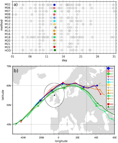
Table 1. List of cyclone tracking methods used in this study according to the IMILAST project denominations (Code M02–M22, HOD), main references of the method description and main variable used

Code	Main references for method description	Main variable used
M02	Murray and Simmonds (1991), Pinto et al. (2005)	MSLP (min), VORT
M06	1997), Hewson and Titley (2010)	MSLP (min. grad.)
M07	Flaounas et al. (2014)	Z850 VORT
M08	2006)	MSLP (min. grad.)
M09	1995), Wang et al. (2006)	MSLP (min. grad.), VORT
M10	Murray and Simmonds (1991), Simmonds et al. (2003)	MSLP (min), VORT
M12	2002), Rudeva and Gulev (2007)	MSLP (min)
M14	Kew et al. (2010)	Z850 (min. contour)
M15	Blender et al. (1997), Raible et al. (2008)	MSLP (min)
M16	2002)	MSLP (min)
M18	1994, Sinclair 1997)	Z850 VORT
M20	2006)	MSLP (min)
M21	2009)	Z850 VORT
M22	2005), Akperov et al. (2007)	MSLP (min. contour)
HOD	Hodges (1994, 1999), Hodges et al. (2011)	Z850 VORT

MSLP, mean sea level pressure; VORT, vorticity or Laplacian of MSLP; Z850 VORT, vorticity at 850 hPa; Z850, geopotential height at 850 hPa; grad., gradient of MSLP; min, minimum.

2.2. Quantification of clustering

The occurrence of random events in time can be represented by the homogeneous Poisson process (Cox and Isham, 1980). If the events (cyclones) arise with a rate of occurrence λ, then the number of events y in a time interval T is Poisson distributed (random), with mean () and sample variance () both equal to λT, and thus =1. Deviations from the Poisson process indicate a non-random arrival of cyclones over time, in the sense that events systematically occur in a more clustered (in groups) or a more regular way (equal spacing in time; cf. Supplementary Fig. S1). These deviations from the Poisson process can be used to assess the degree of clustering, and following Mailier et al. (2006), we use the dispersion statistic:1

A Poisson process (=) with a constant rate of occurrence λ implies φ=0. Positive values of φ indicate clustering (overdispersion; >), and negative values of φ indicate regularity (underdispersion; <; cf. Supplementary Fig. S1). Following Pinto et al. (2013), events are defined as cyclone tracks intercepting a radius of influence around a certain grid point. An identification radius of 700 km was selected based on considerations related to cyclone sizes and potential impacts, so the rate is the number of cyclones that pass through this region with an area of π·700 km² (see Pinto et al., 2013 for more details). When a cyclone track intercepts the circle for a selected grid point, the time corresponding to the nearest position to the circle centre is counted (cf. Fig. 1a for an example). In this way, time series are obtained for each method (Fig. 1b). This approach is applied at each location (grid point) and was recently used to estimate clustering of cyclones simulated by CMIP5 global climate models (Economou et al., 2015). For each winter (DJF), cyclone counts (y _i ) are computed for the period 1979/1980–2009/2010 to produce a time series of counts {y ₁,y ₂,…y _n} at each grid point, where n is the number of winters.

2.3. Relationship with the NAO

As explained in Economou et al. (2015), overdispersion can be approximated by2

where is the sample variance of , and thus3

The square root transformation stabilises the variance, that is, removes the dependence between mean and variance. Economou et al. (2015) showed that this also allows a regression of on the NAO, in order to quantify the possible influence of the NAO on dispersion:4

where x is the seasonal mean of NAO. The NAO index is calculated following the methodology by Barnston and Livezey (1987), which is based on rotated principal component analysis. The monthly time series for DJF were provided by the Climate Prediction Center from the National Oceanic and Atmospheric Administration and averaged for each winter (DJF).

Parameters α and β in eq. (4) are estimated from the data and represent the intercept and slope parameters of the assumed linear relationship between and the NAO. The term ɛ represents the error about the straight line and is assumed to follow a normal distribution with variance σ ², which is also estimated from the data. To investigate whether the assumption that NAO is linearly related to holds across all methods, we have additionally implemented an extended regression assuming a quadratic relationship:5

The estimated linear and quadratic relationships for two exemplary grid points near the Azores and Iceland are shown in Supplementary Figs. S2 and S3. In general, these plots indicate that there is no real difference between the linear and quadratic fits, so that the linear fit is retained.

Using eq. (4), it can be shown that6

where (s _x )² is the sample variance of the NAO-index x. This allows to diagnose how much of the underdispersion can attribute to modulation of counts by NAO (the parameter β).

3. Quantification of cyclone passages on a grid point basis

Time series of cyclone counts for all 15 methods are first analysed at each grid point. As an example, we consider the grid point 55°N, 5°W centred over the British Isles and cyclone counts for January 2007 (Fig. 1), a period characterised by a large number of storms over this area (Pinto et al., 2014). The corresponding 700 km identification radius is shown in Fig. 1b. The cyclone passages within this area are indicated in the time line (Fig. 1a) and show some similarities but also differences for the individual methods: for example, the number of identified cyclones for this grid point and month ranges from 5 (M22) to 25 (M18). On the other hand, the main cyclones passing through this area (9, 10, 12, 13, 15, 18 and 20 January; cf. Pinto et al., 2014, their Fig. 3) are captured by most methods. Figure 1b shows the individual tracks for all methods for the cyclone passing on 13 January (named storm ‘Hanno’ by the Free University of Berlin). The tracks show generally a good agreement for all methods in the main development phase, when all tracks are found within a corridor of a few hundred kilometres. Small differences between the tracks at this development stage are typical, given that the methods use different key variables for tracking: for example, the MLSP minima and 850 hPa vorticity maxima do not exactly overlap in an extratropical cyclone (e.g. Pinto et al., 2005, their Fig. 1), with the vorticity maxima (e.g. M07, M18 and HOD) typically being located south of the former (e.g. M02 and M06). Less agreement is found at the beginning (different starting points) and particularly at the end of the cyclone tracks, which show diverging trajectories over Eastern Europe: while most methods show a zonal track towards southern Finland and further into northern Russia, some of the vorticity methods (green) show a track towards the Caspian Sea. Similar results have been found in previous case studies analysed in the IMILAST project (Neu et al., 2013, their Figs. 4 and 5).

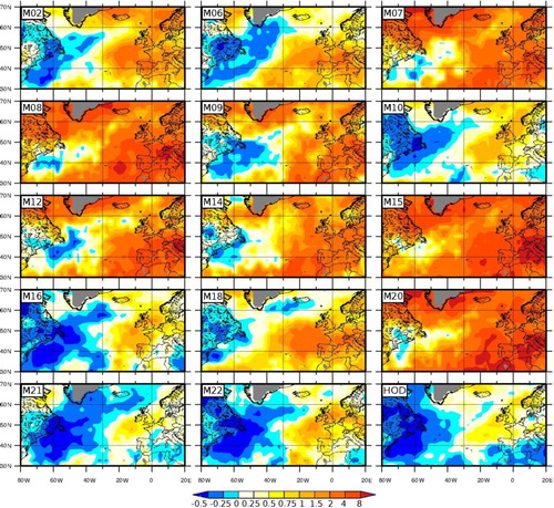
Following this methodology, time series of cyclone counts are derived for each grid point in the domain 30°N–70°N and 80°W–20°E and for the whole study period (winters 1979/1980 to 2009/2010). The mean of counts and their variance (s _y )², the two components needed to estimate φ, are displayed in Figs. 2 and 3 for all 15 cyclone tracking methods. The number of tracks passing through a certain area (; Fig. 2) is comparable to a cyclone track density field and depicts higher magnitudes in areas with many transient cyclones. This is unlike cyclone count statistics, in which cyclones can be counted multiple times in the same location (cf. Pinto et al., 2005). Therefore, some intrinsic differences are found between our Fig. 2 and Fig. 1 from Neu et al. (2013), which shows cyclone count statistics. We have thus identified a larger discrepancy between the algorithms compared to Neu et al. (2013), for example, there is no common peak south of Greenland for all methods (Fig. 2).

Fig. 2 Average number of DJF cyclone passages for each of the 15 methods (M02–M22, HOD) derived from ERA-Interim (1979–2010).

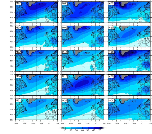
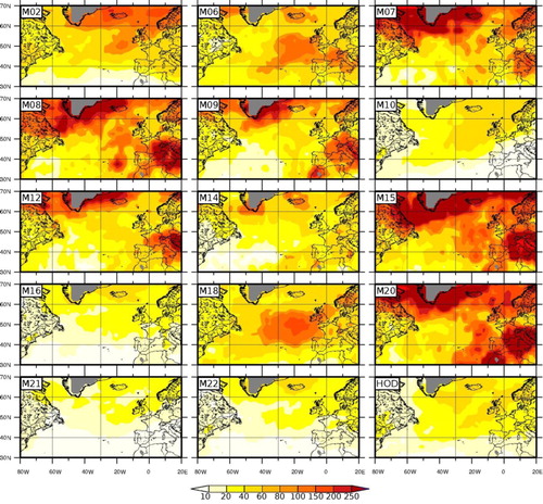
Fig. 3 Variance of DJF cyclone passages (s _y )² for each of the 15 methods (M02–M22, HOD) derived from ERA-Interim (1979–2010).

Differences between tracking methods are identified in Fig. 2 both in terms of total numbers, position of the North Atlantic storm track and regional aspects such as Mediterranean cyclones: for example, methods M14, M21 and M22 show generally small cyclone numbers and relatively weak activity over the Mediterranean basin (Fig. 2). This is not the case for other methods such as M02, M06, M15 and M20. However, the general spatial pattern in mean counts over the North Atlantic storm track qualitatively agrees between methods. Some of the spatial differences between methods can be explained by the choice of variable used in the tracking. For example, cyclone tracks based on 850 hPa vorticity (VORT) are typically displaced southwards to cyclone tracks derived from MSLP minimum (compare M15 and M18). Systematic discrepancies between the various cyclone track algorithms also play a role for the identified differences. See also Neu et al. (2013) for more details. Specific differences within the Mediterranean basin are discussed in Lionello et al. (2016) and will not be further analysed here.

The variance of counts (s _y )² shows more diverse results (Fig. 3). Spatial patterns typically display a maximum of activity south of Greenland, which often extends towards Northern Europe. However, the relative maximum over Western/Central Europe is not found for some methods (e.g. M16 and M21) or is displaced in others (e.g. M06 and M18) to around 50°N–55°N over the eastern North Atlantic. While this relative maximum is also found for other methods (e.g. M02 and M15), it is not the dominant feature. In terms of numbers, the differences in (s _y )² between methods are even larger than for , with values differing by an order of magnitude in some areas, for example, south of Greenland.

4. Quantification of clustering

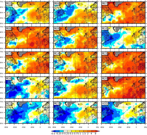
The estimates of φ for the different methods are shown in Fig. 4. The general spatial pattern qualitatively agrees between tracking methods: an area of φ<0 identified over the western North Atlantic (regularity or underdispersion; blue colour), while φ>0 (clustering or overdispersion; red colour) is found on northern and southern flanks and the downstream region of the North Atlantic storm track (compare Mailier et al., 2006 and Pinto et al., 2013). Considering the whole study area, overdispersion (red) tends to dominate for some methods (e.g. M15 and M20), while underdispersion (blue) dominates for others (e.g. M21 and M22). However, most methods show a balance between the two features (e.g. M02, M06 and M18), in line with previous works (Mailier et al., 2006; Pinto et al., 2013). While all methods show overdispersion over Western Europe, the magnitude of φ clearly differs between methods. For the example grid point 55°N, 5°W, φ is positive for all methods (clustering), but ranges from 0.27 (M21) to 4.73 (M20). Differences appear to be dominated primarily by the variance of winter counts (cf. Fig. 3).

Fig. 4 Dispersion statistic φ for each of the 15 methods (M02–M22, HOD) derived from ERA-Interim (1979–2010).

To provide further insight into the differences between methods, we analyse in detail the relations between and (s _y )² for 55°N, 5°W. In Fig. 5, the mean is plotted against the variance, and the lines corresponding to φ=0, 1, 2, 3, 4 and 5 are shown for orientation. Half of the methods are found in the range between φ=0.86 and 1.32, and four methods around 2.0 (M07, M08, M09, M14). Methods M15, M20 and M21 are outliers: the two former methods (both based on MSLP) display a much higher (s _y )² compared to , while for the latter (s _y )² and are small and roughly equal.

The statistical significance bounds for the Poisson distribution (φ=0) is estimated using parametric bootstrapping: 10 000 time series of 30 counts are generated for each mean value (1–55) assuming a Poisson distribution. For each mean value, the empirical 95% quantile of those 10 000 variance values is used to construct a 95% confidence interval (grey area around φ=0 in Fig. 5). This implies that dispersion values for all but two methods (M21, HOD) significantly deviate from Poisson. Similar results are found for other grid points over the eastern North Atlantic and Western Europe (not shown), revealing the robustness of overdispersion of cyclone counts for this area.

Fig. 5 Variance (y-axis) and mean of cyclone track counts per winter (x-axis) for the grid point 55°N, 5°W for each method (M02–M22, HOD). Isolines of dispersion statistic φ are depicted in black (for values 0–5). The grey area depicts a 95% (bootstrap) confidence interval for the variance, under the assumption of no overdispersion.

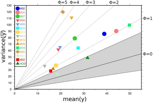
The range of the horizontal axis (in Fig. 5), which shows the mean, is much smaller than the range of the vertical axis, which shows the variance. This indicates that differences in (s _y )² are the primary driver behind the differences in φ. For example, is actually quite similar for M20 and M21 (20.9 and 18.5, respectively), while (s _y )² and thus φ are very different. On the other hand, the consistency of results between M02 and M10 is noteworthy: these approaches basically use the same tracking method with different parameters and provide very similar values of φ (1.21 and 1.32) despite the differences in . Methods displaying underdispersion over most of the study area (e.g. M21 and M22) typically have a small number of cyclone counts (cf. Fig. 2), but the dominant factor for the differences in φ remains (s _y )². It is noteworthy that the two methods with the highest φ values (M15 and M20) are MSLP minimum methods (orange/brown). However, other MSLP minimum methods (M12 and M16) show values closer to the other approaches. It is therefore difficult to associate the diversity of φ results with particular features of tracking methods. This result is consistent with the conclusions of Neu et al. (2013) and Rudeva et al. (2014) regarding cyclone characteristics and their possible dependence on the tracking method.

5. Relationship with the NAO

The recent study by Economou et al. (2015) showed that a considerable part of the overdispersion identified based on ERA-Interim reanalysis cyclone tracks derived with the HOD approach is due to the modulation of cyclone counts by the NAO. In order to investigate the NAO influence on cyclone clustering, dispersion is now quantified following Economou et al. (2015), where φ is approximated by −1 [eq. (2)]. Results are shown in Fig. 6 for each tracking method. The two estimation methods for φ are very similar (compare Figs. 4 and 6), implying that the is a good approximation to φ. In the following, we use this approximation to estimate the contribution of the NAO index to the dispersion index according to eq. (6).

Fig. 6 Estimated dispersion statistic quantified with −1 for each of the 15 methods (M02–M22, HOD) derived from ERA-Interim (1979–2010). Derived from ERA-Interim (1979–2010).

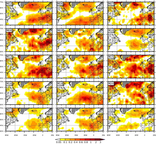
The linear relationship between the strength of the NAO and is quantified by the parameter β. The result is a dipolar structure, revealing a positive pole near Iceland and a negative pole over the Azores (cf. Fig. 7). This systematic influence of the NAO phase on clustering can now be quantified as 4β ²(s _x )² [eq. (6)]. Figure 8 shows the NAO contribution for each method, revealing two maxima, one north and one south of the North Atlantic storm track. This general spatial pattern is in good agreement with Economou et al. (2015) who considered cyclone tracks derived with HOD method and ERA-40 data (Uppala et al., 2005). The North Atlantic storm track moves latitudinally depending on the NAO phase, leading to the two maxima of NAO influence on clustering on the flanks of the storm track.

Fig. 7 Regression coefficient β (see EQ.3) for each of the 15 methods (M02–M22, HOD) derived from ERA-Interim (1979–2010).

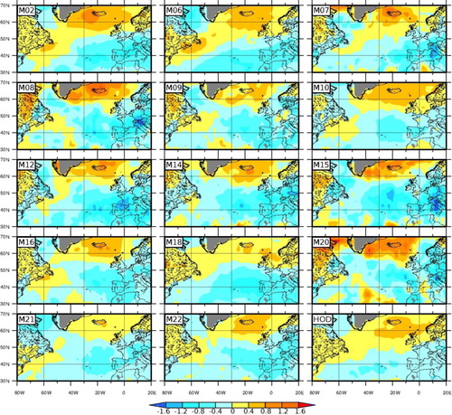
Fig. 8 Effect of North Atlantic Oscillation (NAO) on dispersion following 4β ²(s _x )² for each of the 15 methods (M02–M22, HOD) derived from ERA-Interim (1979–2010).

However, there are differences in the detail between the 15 methods, both in terms of spatial pattern and magnitude. This can be partly explained by the relationship between the NAO influence on dispersion and the magnitude of dispersion itself per method (compare Figs. 4 and 8). For example, a strong influence of the NAO on the clustering of cyclones is found in regions and methods where overdispersion is high (compare Figs. 4 and 8 for M07, M08, M15 and M20 near the Alps). The spatial pattern of NAO influence also shows some differences over Europe: for example, while the region with low NAO influence (white) is located over Northern Europe for most methods, a few methods have this region over Central Europe (M10, M18) or over France (M20). The spatial variability of the NAO influence is high for some methods (M07, M08, M15 and M20), which indicates a larger uncertainty of the β estimate. In general, it is difficult to associate the different types of methods (e.g. using vorticity or MSLP as the cyclone tracking variable) with a specific type of behaviour regarding the NAO influence on cyclone clustering over the North Atlantic and Europe, but the general agreement between the methods is encouraging.

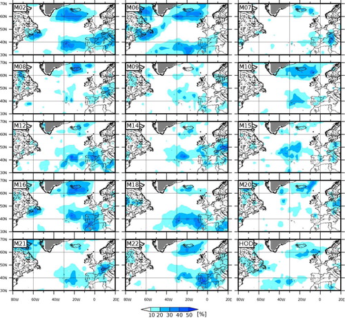
The large differences in the number of counts between the methods lead to strong differences in β and therefore also on the absolute contribution of the NAO to overdispersion. As all the effects contributing to clustering can be quantified as 4β ²(s _x )²+4σ² [eq. (6)], the relative contribution of the NAO is defined as 4β ²(s _x )²/(4β ²(s _x )²+4σ²) and shown in Fig. 9. A similar pattern to Fig. 8 is revealed, with the two maxima near Iceland and the Azores, plus additional maxima over Central Europe or near Newfoundland. The relative contribution of the NAO to clustering exceeds 50% for some methods, particularly south of Iceland and in the region between Azores and Iberia. The intensity and extension of the area around each of the two maxima differ. For example, for M02 both maxima are approximately equally strong, while for M18 the southern maximum is more pronounced. This suggests a stronger (weaker) contribution of other processes than the NAO to the clustering for one (other) maximum. Comparing the Figs. 3 and 9, it is quite apparent that there is no clear link between the difference in variance between methods and the sensitivity to the NAO.

Fig. 9 Relative effect of North Atlantic Oscillation (NAO) on dispersion following for each of the 15 methods (M02–M22, HOD) derived from ERA-Interim (1979–2010).

6. Conclusions

The main objective of this article was to assess if the cyclone clustering over the eastern North Atlantic and Europe is a robust feature using results from 15 cyclone tracking methods. A second objective was to evaluate whether the relationship between NAO and clustering depends on the choice of the tracking method. The main findings of this study are as follows:

• The general spatial pattern of the cyclone dispersion statistic (φ), as previously identified with single tracking methods, is qualitatively captured by all methods: underdispersion (regularity) is identified near the core of the North Atlantic storm track near Newfoundland, while overdispersion (clustering) can be found over the eastern North Atlantic and Western Europe, particularly on both sides and downstream of the North Atlantic storm track.

• Quantitative differences in the values of φ are identified between methods. Some methods display predominantly underdispersion (regularity) over the study area, while others indicate overdispersion (clustering) over almost the whole study area.

• The differences in φ can be primarily attributed to the differences in the variance of cyclone counts between the methods.

• Significant overdispersion is identified for almost all methods over parts of the eastern North Atlantic and Western Europe, indicating the robustness of cyclone clustering in this area. Still, the magnitude of φ may vary strongly between methods.

• The statistical link between NAO and clustering of cyclone tracks is found for all methods and is thus a robust feature: in accordance with previous studies, maxima on both sides of the main storm track are identified, though with slightly different magnitudes and spatial extension.

• The explained variance of the NAO on clustering exceeds 50% for some tracking methods and locations. The differences in the variance of cyclone counts cannot be attributed to different sensitivities to the NAO.

We conclude that both the general pattern of underdispersion and overdispersion over the North Atlantic and Western Europe and the dipolar pattern of NAO influence on dispersion are largely independent from the choice of tracking method and hence from the definition of a cyclone. In particular, overdispersion of cyclone counts is identified for all methods over Western Europe and can therefore be considered as a robust feature. This is an important and valuable information for stakeholders, such as the insurance industry, for whom the clustering of extreme cyclones is a major economic risk.

The present results suggest that estimates of cyclone clustering obtained with single tracking methods can be regarded as qualitatively representative for a wider range of tracking methods. This is particularly important because cyclone clustering may change under future climate conditions (Pinto et al., 2013). Given the large sampling uncertainty, such potential changes may not be detectable in single 30-yr climate model simulations (Economou et al., 2015). Still, Karremann et al. (2014) has recently provided evidence based on a large ensemble of simulations with a single global circulation model that cumulative annual losses associated with extratropical cyclones may increase over most of Europe in future decades due to a combination of changes in potential loss magnitude and changes in storm clustering.

Future research could analyse differences between tracking methods also in higher resolution reanalysis data sets such as NASA-MERRA (Rienecker et al., 2011). The higher spatial and temporal resolution will permit a better quantification of the features identified here and a more detailed dynamical analysis similar to Pinto et al. (2014). Another interesting line of research is to quantify the role of the jet location and intensity for cyclone clustering across Western Europe. Preliminary results (for the grid point 55°N, 5°W) indicate that winters with a stronger jet also have a higher number of counts for all methods, particularly when the jet is located around 45°N–50°N (not shown). Finally, it will be interesting to investigate clustering of extratropical cyclones in global circulation models in more detail, taking into account how cyclones and cyclone clustering are represented at different resolutions, evaluating the representation of the associated physical processes, and analysing how results depend on the tracking method.

7. Acknowledgements

The authors thank Swiss Re for sponsoring the Intercomparison of Mid-Latitude Storm Diagnostics (IMILAST) project. TE and DBS were supported by NERC project CREDIBLE. We thank the open access fund of the University of Reading for support. The authors thank the European Center of Medium Range Weather Forecast (ECMWF, www.ecmwf.int) for the ERA-Interim reanalysis, and the Climate Prediction Center from the National Oceanic and Atmospheric Administration for the NAO index (www.cpc.ncep.noaa.gov/products/precip/CWlink/pna/nao.shtml). The authors thank all the members of the IMILAST project (www.proclim.ch/imilast) for making the cyclone tracks available. We thank Kevin Hodges for making the cyclone tracks available for this study and for discussions. This article profited from discussion with various members of the IMILAST project group. We are thankful to the two anonymous reviewers for their valuable comments and suggestions on a previous version of this article.

Notes

To access the supplementary material to this article, please see Supplementary files under ‘Article Tools’.

References

- Akperov M. G., Bardin M. Y., Volodin E. M., Golitsyn G. S., Mokhov I. I. Probability distributions for cyclones and anticyclones from the NCEP/NCAR reanalysis data and the INM RAS climate model. Izvest. Atmos. Ocean Phys. 2007; 43: 705–712. DOI: http://dx.doi.org/10.1134/S0001433807060047.
- Bardin M. Y. , Polonsky A. B . North Atlantic Oscillation and synoptic variability in the European-Atlantic region in winter. Izvest. Atmos. Ocean Phys. 2005; 41: 127–136.
- Barnston A. G., Livezey R. E. Classification, seasonality and persistence of low-frequency atmospheric circulation patterns. Mon. Weather Rev. 1987; 115: 1083–1126. DOI: http://dx.doi.org/10.1175/1520-0493(1987)115<1083:CSAPOL>2.0.CO;2.
- Blender R., Fraedrich K., Lunkeit F. Identification of cyclone track regimes in the North Atlantic. Q. J. Roy. Meteorol. Soc. 1997; 123: 727–741. DOI: http://dx.doi.org/10.1002/qj.49712353910.
- Blender R., Raible C. C., Lunkeit F. Non-exponential return time distributions for vorticity extremes explained by fractional Poisson processes. Q. J. Roy. Meteorol. Soc. 2015; 141: 249–257. DOI: http://dx.doi.org/10.1002/qj.2354.
- Bjerknes J. , Solberg H . Life cycle of cyclones and the polar front theory of atmospheric circulation. Geofys. Publ. 1922; 3: 3–18.
- Cox D. R. , Isham V . Point Processes. 1980; Chapman and Hall/CRC, London. 188.
- Dee D. P., Uppala S. M., Simmons A. J., Berrisford P., Poli P, co-authors. The ERA-Interim reanalysis: configuration and performance of the data assimilation system. Q. J. Roy. Meteorol. Soc. 2011; 137: 553–597. DOI: http://dx.doi.org/10.1002/qj.828.
- Economou T., Stephenson D. B., Ferro C. A. T. Spatio-temporal modelling of extreme storms. Ann. Appl. Stat. 2014; 8: 2223–2246. DOI: http://dx.doi.org/10.1214/14-AOAS766.
- Economou T., Stephenson D. B., Pinto J. G., Shaffrey L. C., Zappa G. Serial clustering of extratropical cyclones in historical and future CMIP5 model simulations. Q. J. Roy. Meteorol. Soc. 2015; 141: 3076–3087. DOI: http://dx.doi.org/10.1002/qj.2591.
- Flaounas E., Kotroni V., Lagouvardos K., Flaounas I. CycloTRACK (v1.0): tracking winter extratropical cyclones based on relative vorticity: sensitivity to data filtering and other relevant parameters. Geosci. Model Dev. 2014; 7: 1841–1853. DOI: http://dx.doi.org/10.5194/gmd-7-1841-2014.
- Gómara I., Pinto J. G., Woollings T., Masato G., Zurita-Gotor P, co-authors. Rossby wave-breaking analysis of explosive cyclones in the Euro-Atlantic sector. Q. J. Roy. Meteorol. Soc. 2014; 140: 738–753. DOI: http://dx.doi.org/10.1002/qj.2190.
- Hanley J., Caballero R. The role of large-scale atmospheric flow and Rossby wave breaking in the evolution of extreme windstorms over Europe. Geophys. Res. Lett. 2012; 39 L21708. DOI: http://dx.doi.org/10.1029/2012GL053408.
- Hewson T. D. Objective identification of frontal wave cyclones. Meteorol. Appl. 1997; 4: 311–315. DOI: http://dx.doi.org/10.1017/S135048279700073X.
- Hewson T. D., Neu U. Cyclones, windstorms and the IMILAST project. Tellus A. 2015; 67 27128. DOI: http://dx.doi.org/10.3402/tellusa.v67.27128.
- Hewson T. D., Titley H. A. Objective identification, typing and tracking of the complete lifecycles of cyclonic features at high spatial resolution. Meteorol. Appl. 2010; 17: 355–381. DOI: http://dx.doi.org/10.1002/met.204.
- Hodges K. I. A general method for tracking analysis and its application to meteorological data. Mon. Weather Rev. 1994; 122: 2573–2585. DOI: http://dx.doi.org/10.1175/1520-0493(1994)122<2573:AGMFTA>2.0.CO;2.
- Hodges K. I. Adaptive constraints for feature tracking. Mon. Weather Rev. 1999; 127: 1362–1373. DOI: http://dx.doi.org/10.1175/1520-0493(1999)127<1362:ACFFT>2.0.CO;2.
- Hodges K. I., Lee R. W., Bengtsson L. A comparison of extratropical cyclones in recent reanalyses ERA-Interim, NASA MERRA, NCEP CFSR, and JRA-25. J. Clim. 2011; 24: 4888–4906. DOI: http://dx.doi.org/10.1175/2011JCLI4097.1.
- Hoskins B. J., Hodges K. I. New perspectives on the Northern Hemisphere winter storm tracks. J. Atmos. Sci. 2002; 59: 1041–1061. DOI: http://dx.doi.org/10.1175/1520-0469(2002)059<1041:NPOTNH>2.0.CO;2.
- Hunter A., Stephenson D. B., Economou T., Holland M., Cook I. New perspectives on the aggregated risk of extratropical cyclones. Q. J. Roy. Meteorol. Soc. 2016; 142: 243–256. DOI: http://dx.doi.org/10.1002/qj.2649.
- Huntingford C., Marsh T., Scaife A. A., Kendon E. J., Hannaford J., co-authors. Potential influences in the United Kingdom's floods of winter 2013–2014. Nat. Clim. Change. 2014; 4: 769–777. DOI: http://dx.doi.org/10.1038/nclimate2314.
- Hurrell J. W., Kushnir Y., Ottersen G., Visbeck M. An overview of the North Atlantic Oscillation. The North Atlantic Oscillation: Climatic Significance and Environmental Impact. 2003. (eds. J. W. Hurrell, Y. Kushnir, G. Ottersen and M. Visbeck), American Geophysical Union, Washington, DC, pp. 1–35. DOI: http://dx.doi.org/10.1029/134GM01.
- Inatsu M. The neighbor enclosed area tracking algorithm for extratropical wintertime cyclones. Atmos. Sci. Lett. 2009; 10: 267–272. DOI: http://dx.doi.org/10.1002/asl.238.
- Karremann M. K., Pinto J. G., Reyers M., Klawa M. Return periods of losses associated with European windstorm series in a changing climate. Environ. Res. Lett. 2014; 9 124016. DOI: http://dx.doi.org/10.1088/1748-9326/9/12/124016.
- Kew S. F., Sprenger M., Davies H. C. Potential vorticity anomalies of the lowermost stratosphere: a 10-yr winter climatology. Mon. Weather Rev. 2010; 138: 1234–1249. DOI: http://dx.doi.org/10.1175/2009MWR3193.1.
- Lionello P., Dalan F., Elvini E. Cyclones in the Mediterranean region: the present and the doubled CO2 climate scenarios. Clim. Res. 2002; 22: 147–159. DOI: http://dx.doi.org/10.3354/cr022147.
- Lionello P., Trigo I. F., Gil V., Liberato M. L. R., Nissen K. M., co-authors. Objective climatology of cyclones in the Mediterranean region: a consensus view among methods with different system identification and tracking criteria. Tellus A. 2016; 68 29391. DOI: http://dx.doi.org/10.3402/tellusa.v68.29391.
- Mailier P. J., Stephenson D. B., Ferro C. A. T., Hodges K. I. Serial clustering of extratropical cyclones. Mon. Weather Rev. 2006; 134: 2224–2240. DOI: http://dx.doi.org/10.1175/MWR3160.1.
- Matthews T., Murpy C., Wilby R. L., Harrigan S. Stormiest winter on record for Ireland and UK. Nat. Clim. Change. 2014; 4: 738–740. DOI: http://dx.doi.org/10.1038/nclimate2336.
- Messori G., Caballero R. On double Rossby wave breaking in the North Atlantic. J. Geophys. Res. Atmos. 2015; 120: 11129–11150. DOI: http://dx.doi.org/10.1002/2015JD023854.
- Murray R. J. , Simmonds I . A numerical scheme for tracking cyclone centres from digital data. Part I: development and operation of the scheme. Aust. Meteorol. Mag. 1991; 39: 155–166.
- Neu U., Akperov M. G., Bellenbaum N., Benestad R., Blender R., co-authors. IMILAST – a community effort to intercompare extratropical cyclone detection and tracking algorithms: assessing method-related uncertainties. Bull. Am. Meteorol. Soc. 2013; 94: 529–547. DOI: http://dx.doi.org/10.1175/BAMS-D-11-00154.1.
- Parker D. J. Secondary frontal waves in the North Atlantic region: a dynamical perspective of current ideas. Q. J. Roy. Meteorol. Soc. 1998; 124: 829–856. DOI: http://dx.doi.org/10.1002/qj.49712454709.
- Pinto J. G., Bellenbaum N., Karremann M. K., Della-Marta P. M. Serial clustering of extratropical cyclones over the North Atlantic and Europe under recent and future climate conditions. J. Geophys. Res. Atmos. 2013; 118: 12476–12485. DOI: http://dx.doi.org/10.1002/2013JD020564.
- Pinto J. G., Gómara I., Masato G., Dacre H. F., Woollings T., co-authors. Large-scale dynamics associated with clustering of extra-tropical cyclones affecting Western Europe. J. Geophys. Res. Atmos. 2014; 119: 13704–13719. DOI: http://dx.doi.org/10.1002/2014JD022305.
- Pinto J. G., Raible C. C. Past and recent changes in the North Atlantic oscillation. Wiley Interdisc. Rev. Clim. Change. 2012; 3: 79–90. DOI: http://dx.doi.org/10.1002/wcc.150.
- Pinto J. G., Spangehl T., Ulbrich U., Speth P. Sensitivities of a cyclone detection and tracking algorithm: individual tracks and climatology. Meteorol. Z. 2005; 14: 823–838. DOI: http://dx.doi.org/10.1127/0941-2948/2005/0068.
- Pinto J. G., Zacharias S., Fink A. H., Leckebusch G. C., Ulbrich U. Factors contributing to the development of extreme North Atlantic cyclones and their relationship with the NAO. Clim. Dynam. 2009; 32: 711–737. DOI: http://dx.doi.org/10.1007/s00382-008-0396-4.
- Raible C. C., Della-Marta P., Schwierz C., Wernli H., Blender R. Northern Hemisphere extratropical cyclones: a comparison of detection and tracking methods and different reanalyses. Mon. Weather Rev. 2008; 136: 880–897. DOI: http://dx.doi.org/10.1175/2007MWR2143.1.
- Rienecker M. M., Suarez M. J., Gelaro R., Todling R., Bacmeister J., co-authors. MERRA: NASA's modern-era retrospective analysis for research and applications. J. Clim. 2011; 24: 3624–3648. DOI: http://dx.doi.org/10.1175/JCLI-D-11-00015.1.
- Rudeva I., Gulev S. K. Climatology of cyclone size characteristics and their changes during the cyclone life cycle. Mon. Weather Rev. 2007; 135: 2568–2587. DOI: http://dx.doi.org/10.1175/MWR3420.1.
- Rudeva I., Gulev S. K., Simmonds I., Tilinina N. The sensitivity of characteristics of cyclone activity to identification procedures in tracking algorithms. Tellus A. 2014; 66 24961. DOI: http://dx.doi.org/10.3402/tellusa.v66.24961.
- Serreze M. C. Climatological aspects of cyclone development and decay in the Arctic. Atmos. Ocean. 1995; 33: 1–23. DOI: http://dx.doi.org/10.1080/07055900.1995.9649522.
- Simmonds I., Keay K., Lim E.-P. Synoptic activity in the seas around Antarctica. Mon. Weather Rev. 2003; 131: 272–288. DOI: http://dx.doi.org/10.1175/1520-0493(2003)131<0272:SAITSA>2.0.CO;2.
- Sinclair M. R. An objective cyclone climatology for the Southern Hemisphere. Mon. Weather Rev. 1994; 122: 2239–2256. DOI: http://dx.doi.org/10.1175/1520-0493(1994)122<2239:AOCCFT>2.0.CO;2.
- Sinclair M. R. Objective identification of cyclones and their circulation intensity, and climatology. Weather Forecast. 1997; 12: 595–612. DOI: http://dx.doi.org/10.1175/1520-0434(1997)012<0595:OIOCAT>2.0.CO;2.
- Trigo I. F. Climatology and interannual variability of storm-tracks in the Euro-Atlantic sector: a comparison between ERA-40 and NCEP/NCAR reanalyses. Clim. Dynam. 2006; 26: 127–143. DOI: http://dx.doi.org/10.1007/s00382-005-0065-9.
- Uppala S. M., Källberg P. W., Simmons A. J., Andrae U., Bechtold V. D. C., co-authors. The ERA-40 re-analysis. Q. J. Roy. Meteorol. Soc. 2005; 131: 2961–3012. DOI: http://dx.doi.org/10.1256/qj.04.176.
- Vitolo R., Stephenson D. B., Cook I. M., Mitchell-Wallace K. Serial clustering of intense European storms. Meteorol. Z. 2009; 18: 411–424. DOI: http://dx.doi.org/10.1127/0941-2948/2009/0393.
- Wang X. L., Swail V. R., Zwiers F. W. Climatology and changes of extratropical cyclone activity: comparison of ERA-40 with NCEP-NCAR reanalysis for 1958–2001. J. Clim. 2006; 19: 3145–3166. DOI: http://dx.doi.org/10.1175/JCLI3781.1.
- Wernli H., Schwierz C. Surface cyclones in the ERA-40 dataset (1958–2001). Part I: novel identification method and global climatology. J. Atmos. Sci. 2006; 63: 2486–2507. DOI: http://dx.doi.org/10.1175/JAS3766.1.
- Zolina O., Gulev S. K. Improving the accuracy of mapping cyclone numbers and frequencies. Mon. Weather Rev. 2002; 130: 748–759. DOI: http://dx.doi.org/10.1175/1520-0493(2002)130<0748:ITAOMC>2.0.CO;2.