Comparative CO₂ flux measurements by eddy covariance technique using open- and closed-path gas analysers over the equatorial Pacific Ocean

Abstract

Direct comparison of air–sea CO₂ fluxes by open-path eddy covariance (OPEC) and closed-path eddy covariance (CPEC) techniques was carried out over the equatorial Pacific Ocean. Previous studies over oceans have shown that the CO₂ flux by OPEC was larger than the bulk CO₂ flux using the gas transfer velocity estimated by the mass balance technique, while the CO₂ flux by CPEC agreed with the bulk CO₂ flux. We investigated a traditional conflict between the CO₂ flux by the eddy covariance technique and the bulk CO₂ flux, and whether the CO₂ fluctuation attenuated using the closed-path analyser can be measured with sufficient time responses to resolve small CO₂ flux over oceans. Our results showed that the closed-path analyser using a short sampling tube and a high volume air pump can be used to measure the small CO₂ fluctuation over the ocean. Further, the underestimated CO₂ flux by CPEC due to the attenuated fluctuation can be corrected by the bandpass covariance method; its contribution was almost identical to that of H₂O flux. The CO₂ flux by CPEC agreed with the total CO₂ flux by OPEC with density correction; however, both of them are one order of magnitude larger than the bulk CO₂ flux.

• CO₂ flux
• eddy covariance technique
• open-path gas analyser
• closed-path gas analyser
• WPL correction

1. Introduction

Eddy covariance technique is the most direct turbulent flux measurement. This technique makes it possible to measure the flux on the same time and spatial scales as the variability of various processes that influence the trace gas flux between the air–sea interface. However, in this technique, fluxes of only three trace gases, H₂O, CO₂ and CH₄, can be directly measured using an open-path gas analyser (OPGA); the fluxes of other trace gases (SO₂, NO, NO _x , O₃) and a carbon isotope (¹³CO₂) have to be indirectly measured using a closed-path gas analyser (CPGA) in which the sample air must be first drawn through a sampling tube into a sample cell.

Since the first measurement reported by Jones and Smith (1977), the turbulent CO₂ flux directly evaluated by the open-path eddy covariance (OPEC) technique over the coastal sea and open ocean was shown to be larger than the air–sea bulk CO₂ flux estimated using the gas transfer velocity, which was evaluated by mass balance techniques using natural and bomb-produced ¹⁴C, ²²²Rn/²²⁶Ra and SF₆/³He as tracers (Smith and Jones, 1985; Jacobs et al., 1999; Kondo and Tsukamoto, 2007). McGillis et al. (2001, 2004) reported that, in contrast, the turbulent CO₂ flux evaluated by the closed-path eddy covariance (CPEC) technique has shown almost the same value as the bulk CO₂ flux estimated using the gas transfer velocity, which was simultaneously evaluated by a mass balance technique using SF₆/³He dual tracers. Miller et al. (2010) also evaluated the turbulent CO₂ flux by the CPEC, which was converted from an original OPGA and reached the same conclusion as reported in the study by McGillis et al. (2001).

Comparative measurements of CO₂ fluxes by the OPEC and CPEC over the land were performed in the 1990s (Leuning and Moncrieff, 1990), and the results were consistent (Suyker and Verma, 1993; Lee et al., 1994; Yasuda and Watanabe, 2001; Ibrom et al., 2007b). However, over the ocean where the CO₂ density fluctuation is one order of magnitude smaller than that over the terrestrial ecosystem, comparative measurements of CO₂ fluxes using both analysers have rarely been reported.

The OPGA has an advantage of directly measuring the CO₂ density fluctuation in atmospheric turbulence. Considering the present sensitivity of gas analysers used over the ocean where high accuracy measurement is required, it has the other advantage of measuring the larger CO₂ density fluctuation than the fluctuation caused by air–sea CO₂ flux because of including the apparent CO₂ density fluctuation due to the air density fluctuation resulting from the air temperature and H₂O density fluctuations. In the 1970s, when the first measurement was performed (Jones and Smith, 1977), there was a question whether the CO₂ flux evaluated by the eddy covariance technique was sufficiently accurate over the ocean where the CO₂ density fluctuation is small. Recently, Kondo and Tsukamoto (2007) has reported that precise measurements of this small CO₂ density fluctuation using the present OPGA were obtained over the equatorial Indian Ocean based on detailed spectral analysis. However, the magnitude of upward density correction due to air temperature and H₂O density fluctuations the so-called Webb or WPL (Webb, Pearman and Leuning) correction, mentioned in a later section exceeded the apparent downward CO₂ flux. In contrast, the CPGA can indirectly measure the CO₂ density fluctuation in moist sample air, which is influenced by the air density fluctuation due to only the H₂O density fluctuation because the temperature fluctuation in the sample air is fully attenuated in a sampling tube from the sampling point (Sahlée and Drennan, 2009). Moreover, the CPGA can measure the CO₂ density (or mixing ratio) fluctuation in sample air that was pre-dried using a membrane dryer; therefore, it has the advantage of evaluating the CO₂ flux without the WPL correction. However, the CO₂ density fluctuation measured by the CPGA attenuates in the sampling tube. The degree of this attenuation, which leads to underestimations of the CO₂ flux, primarily depends on two factors: the length and diameter (dead volume) of the sampling tube and the airflow state (laminar or turbulent) within the tube (Leuning and Moncrieff, 1990; Lenschow and Raupach, 1991; Leuning and King, 1992). Many researchers have used a high volume air pump to keep the turbulent airflow within the sampling tube. However, the length of sampling tube is required to be long because of the constraints faced on many ships over the open ocean. When using a long sampling tube, the CPGA may not measure the attenuated smaller CO₂ density (or mixing ratio) fluctuation with a sufficient time response to resolve the CO₂ flux when using a long sampling tube to evaluate the small CO₂ flux over the ocean. McGillis et al. (2001) and Miller et al. (2010) used a long sampling tube, but they did not convincingly report whether the attenuated smaller CO₂ density (or mixing ratio) fluctuation over the ocean could be measured by the CPGA.

This study presents a direct comparison of the small CO₂ fluxes by the OPEC and CPEC over the open ocean. A fast Fourier transform spectrum analysis technique was used to demonstrate the attenuating influence of the sampling tube on the CO₂ density fluctuation measured by the CPGA. We also discuss the possibility of the underestimated flux correction (frequency correction) for the attenuated small CO₂ density fluctuation measured by the CPGA. Finally, we present a direct comparison of the CO₂ fluxes evaluated by the eddy covariance technique using both analysers in addition to the bulk CO₂ flux estimated using the gas transfer velocity by the mass balance technique.

2. Methods

2.1. Theory of CO₂ fluxes by the OPEC and CPEC techniques

The air–sea turbulent CO₂ flux by the eddy covariance technique [F _c(EC), mg m⁻² s⁻¹] is given by:1

where ρ _d is the dry air mass density (kg m⁻³), w is the vertical wind velocity (m s⁻¹) and r _c is the mass mixing ratio of CO₂ relative to the dry air (mg kg⁻¹). The prime indicates the fluctuation as a deviation from the mean value (overbar) over a sampling period.

The infrared CO₂/H₂O gas analyser measures the CO₂ and H₂O densities rather than their mixing ratios because it cannot measure the air temperature and pressure at the same time and point in atmospheric turbulence. Therefore, the turbulent CO₂ flux by the eddy covariance technique is given by:2

where ρ _c is the CO₂ mass density (mg m⁻³). The first and second terms on the right-hand side of eq. (2) are the raw CO₂ flux and the CO₂ flux due to the mean vertical flow, respectively. Webb et al. (1980) suggested that the flux due to the mean vertical flow cannot be neglected for trace gases such as H₂O and CO₂. To evaluate the magnitude of the influence of the mean vertical flow, Webb et al. (1980) assumed that the vertical flux of dry air should be zero:3

Using the ideal gas equation, the final expression for the total CO₂ flux by the OPEC technique [F _c(OPEC), mg m⁻² s⁻¹] can be written as follows:4

where ρ _{c_op} and ρ _{v_op} are the CO₂ and H₂O mass densities measured by the open-path CO₂/H₂O gas analyser (mg m⁻³), respectively, µ is the ratio of the molecular weights of dry air to those of H₂O (kg g⁻¹), σ is the ratio of H₂O density to dry air density (g kg⁻¹) and T is the absolute air temperature (K). The first, second and third terms on the right-hand side in eq. (4) are the raw CO₂ flux and WPL correction terms due to H₂O density fluctuations (related to latent heat flux, and hereafter, WPL for LHF) and due to air temperature fluctuations (related to sensible heat flux, and hereafter, WPL for SHF), respectively.

The CO₂ flux by the CPEC technique [F _c(CPEC), mg m⁻² s⁻¹] can be expressed as follows (Leuning and Moncrieff, 1990; Suyker and Verma, 1993):5

where p and T are the air pressure and temperature, respectively, and T _cl, p _cl, ρ _{c_cl} and ρ _{v_cl} are the temperature, pressure and CO₂ and H₂O mass densities in the sample cell of the closed-path CO₂/H₂O gas analyser, respectively. Equation (5) assumes that the temperature fluctuation in the sample air is attenuated (T′=0) when the air is drawn through a sampling tube. In the present study, we have adopted a closed-path CO₂/H₂O infrared gas analyser that gives the CO₂ and H₂O mole fractions as the output; they were calculated from the measured CO₂ and H₂O densities using the pressure and temperature in the sample cell. The CO₂ flux by the CPEC technique is thus given by Yasuda and Watanabe (2001):6 7 8

where ρ _{a_cl} is the moist air mass density in a sample cell (kg m⁻³), X _{c_cl} (µmol mol⁻¹) and X _{v_cl} (mmol mol⁻¹) are the CO₂ and H₂O mole fractions in the moist air in the sample cell measured by the closed-path CO₂/H₂O gas analyser, and m _c, m _d and m _a are the molecular weights of CO₂ (44.01 g mol⁻¹), dry air (28.97 g mol⁻¹) and moist air, respectively.

2.2. Theory of air–sea bulk CO₂ flux

A two-layer film model can be used for the estimation of air–sea gas flux (Liss and Merlivat, 1986). The air–sea bulk CO₂ flux [F _c(Bulk), mg m⁻² s⁻¹] can be calculated from the air–sea difference in the fugacity of CO₂ at the surface and gas transfer velocity as follows:9

where k _c (m s⁻¹) is the gas transfer velocity of CO₂ modified by the Schmidt number, S _c (mg m⁻³ µatm⁻¹) is the solubility of CO₂, which depends on the salinity and seawater temperature (Weiss, 1974) and ΔfCO₂ (µatm) is the difference between the fugacities of CO₂ in bulk seawater and air, respectively. The layer thickness controls the gas transfer velocity and depends significantly on the wind speed. Empirical equations describe the gas transfer velocity as a function of wind speed. Variety parameterisations have been proposed to calculate the gas transfer velocity of CO₂. In this study, we have adopted the gas transfer velocity proposed by Wanninkhof (1992), which was evaluated by the mass balance technique using the tracers of the natural and bomb-produced ¹⁴C, ²²²Rn/²²⁶Ra and SF₆/³He. Wanninkhof (1992) proposed the gas transfer velocity, k _c=0.31 U ², where U is the wind speed. We estimated the bulk CO₂ flux at each station using the mean wind speed and ΔfCO₂ for the period during which flux observation runs were performed.

2.3. Instrumentation

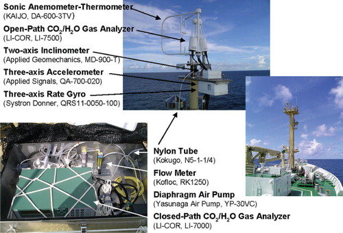
We installed turbulent flux and ship motion correction systems on top of the foremast (approximately 24 m above the mean sea surface) of the R/V MIRAI, as shown in Fig. 1. The turbulent flux system consisted of a sonic anemometer-thermometer (SAT) (KAIJO, DA-600-3TV) for measuring the fluctuations of three wind velocities and sound virtual temperature as well as the infrared open-path (LI-COR, LI-7500) and closed-path (LI-COR, LI-7000) CO₂/H₂O gas analysers for measuring the fluctuations of the CO₂ and H₂O densities and mole fractions, respectively. A diaphragm air pump (Yasunaga Air Pump, YP-30VC) was used to draw the sample air from the sampling point near the OPGA and SAT through a nylon tube (3.2 m long, 1/4 inch in diameter) to the sample cell of the CPGA. In this study, we used a short sampling tube because of focusing on the difference in theory between the CO₂ fluxes by the OPEC and CPEC. The flow rate to the sample cell of CPGA was maintained at 12.0 L min⁻¹ with a mass flow controller (Kofloc, RK1250). The theoretical CPGA lag time for CO₂ and H₂O due to the travel time in the sampling tube, which was calculated from the inner diameter and length of the tube and the flow rate of the air pump, was 0.3 s. On the other hand, the actual CPGA lag times determined by the cross-correlation of signals from both SAT and CPGA were 1.0–1.4 s; the CPGA signals were shifted accordingly. The reference cell in the CPGA was filled with a magnesium perchlorate desiccant and compressed pure air gas at a flow rate of 50 mL min⁻¹ as zero gas. Serrano-Ortiz et al. (2008) reported that the contamination of the optical window of the OPGA results in errors in the absolute measurement of the CO₂ density. Prytherch et al. (2010) suggested that this contamination results in errors not only in the absolute CO₂ density but also in its fluctuation. In this study, we cleaned the LI-7500 optical windows before the observations to avoid contamination by salt particles and raindrops and checked the Automatic Gain Control value (‘clean window’ baseline value) before and after all the special observations presented in the next section. The ship motion correction system consisted of a two-axis inclinometer (Applied Geomechanics, MD-900-T) for measuring the pitching and rolling angles, a three-axis accelerometer (Applied Signals, QA-700-020) for measuring three accelerations and a three-axis rate gyro (Systron Donner, QRS11-0050-100) for measuring three angular rates.

Fig. 1.  Systems for turbulent flux observation and ship motion correlation on top of the foremast of the R/V MIRAI, JAMSTEC during the MR08-03 cruise.

The analogue output signals from these instruments were sampled and digitised at a rate of 100 Hz using analogue-to-digital converters (National Instruments, DAQCard-AI-16XE-50) and recorded at an average rate of 10 Hz using a data acquisition system (National Instruments, LabVIEW 8.5) on a laptop computer. All the data processing were carried out after the observations. The fluxes and spectra by the OPEC and CPEC were calculated at 30-min intervals. The wind velocities measured by the SAT were corrected for ship motion following Takahashi et al. (2005) and were rotated into a coordinate system aligned with the mean wind (McMillen, 1988). The crosswind correction for the sound virtual temperature measured by the SAT was included (Hignett, 1992). A linear de-trending of low frequency was applied to the fluctuation in each parameter before calculating each flux. At high frequencies, the losses in the CO₂ and H₂O fluxes by the OPEC caused by the sensor separation between the OPGA and SAT were corrected by the bandpass covariance method, assuming that the ratio of each high frequency of the cospectrum of the raw CO₂ flux to the sensible heat flux is similar (Watanabe et al., 2000). This method has been attempted by many researchers (e.g. Högström et al., 1989; Verma et al., 1992; Grelle and Lindroth, 1996), and it has been accepted as a good method for correcting both the high-frequency flux losses due to the sensor separation (Ono et al., 2007) and the sampling tubing attenuation (Yasuda and Watanabe, 2001). For that reason, the CO₂ and H₂O flux losses for the CPEC in this study were also corrected using the same method.

The general meteorological data (air temperature, humidity, short- and long-wave radiation, wind speed and direction and air pressure) were measured at a height of approximately 24 m above the sea surface with the Shipboard Oceanographic and Atmospheric Radiation measurement (SOAR) and Surface Meteorological observation (SMET) systems. The properties of the bulk seawater temperature and salinity were measured at a depth of approximately 4.5 m below the sea surface.

The fugacities of CO₂ in the air and bulk seawater were calculated from the seawater temperature, salinity and mole fractions of CO₂ in dry marine air and in dry air equilibrated with seawater, which were measured using an automated system with a closed-path CO₂ gas analyser (Murata and Takizawa, 2003). This automated system was operated in one-and-a-half hour cycles. Standard gasses, marine air and equilibrated air with surface seawater within the equilibrator in one cycle were analysed subsequently. The concentrations of the standard gases were 299.90, 349.99, 399.94 and 449.99 ppmv. The marine air was sampled at approximately 0.5 L min⁻¹ from an inlet approximately 30 m above the sea surface at the bow of the ship. Equilibrated air was sampled at 0.7–0.8 L min⁻¹ from a showerhead-type equilibrator, and the seawater for equilibration was taken from a depth of approximately 4.5 m at 5–6 L min⁻¹. These air were dried with the cooling unit, membrane dryer (Permapure, MD-110-72P) and desiccant holder containing Mg(ClO₄)₂. The precision of sea–air CO₂ fugacity difference (ΔfCO₂) measurements in this study was within 1.9 µatm.

2.4. Observation sites

The observations were conducted aboard the R/V MIRAI of the Japan Agency for Marine-Earth Science and Technology (JAMSTEC) during the MR08-03 cruise in the equatorial Pacific Ocean. The cruise track was from Guam to Sekinehama, and it is shown in Fig. 2. This cruise took place from 3 July 2008 through 6 August 2008. During the MR08-03 cruise, special times for the turbulent flux observation were set at the four stations as shown in Table 1. The first to third runs were performed at station A (147°E, EQ), the fourth run at station B (156°E, 5°S), the fifth run at station C (156°E, EQ) and the sixth run at station D (156°E, 2°N). During these runs, the vessel was steered into the wind at a constant speed of maximum 8 knots to maintain the ship heading and to eliminate ship body effects.

Fig. 2.  Cruise track of the R/V MIRAI during MR08-03. This cruise took place from Guam (3 July 2008) to Sekinehama (6 August 2008), and it performed special observations for the flux measurements by the eddy covariance technique at the four (from A to D) stations.

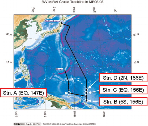
Table 1. Station, position, day time, number (n) of fluxes measured by the eddy covariance technique, and mean values and SDs of wind speed, relative humidity, sea–air temperature difference (ΔT _sea–air) and sea–air CO₂ fugacity difference (ΔfCO₂), during the turbulent flux observation runs performed at the four stations

Station	A			B	C	D
Position (latitude, longtitude)	EQ, 147°E			5°S, 156°E	EQ, 156°E	2°N, 156°E
Run	First	Second	Third	Fourth	Fifth	Sixth
Day time (MM/DD HH:MM)	07/09 12:00–18:00	07/10 07:00–19:00	07/11 08:30–19:30	07/16 07:30–17:30	07/20 07:30–17:30	07/22 07:30–18:00
n	9	15	17	15	18	16
Wind speed (m s^−1)	2.9±0.7	3.5±0.6	4.2±0.3	5.2±0.5	5.4±1.1	2.5±0.7
Relative humidity (%)	75.7±1.9	75.0±1.7	71.3±1.8	77.0±1.1	69.3±1.7	73.9±1.8
ΔT sea–air (°C)	+0.9±0.2	+1.0±0.4	+0.7±0.1	+0.4±0.1	+0.2±0.2	+0.5±0.1
ΔfCO2 (µatm)	+20.5±1.0	+23.9±10	+24.7±0.8	+12.7±1.9	+34.3±0.6	+41.5±0.5

During each flux run, the mean wind speed was low to moderate, ranging from 2.5 to 5.2 m s⁻¹. Sea surface temperature was almost constant and higher than air temperature, and the mean sea–air temperature difference (ΔT _{sea − air}) was small at + 0.2 to + 1.0°C. Relative humidity was also relatively constant during each flux run and had a narrow range from 69.3 to 77.0%. Atmospheric fCO₂ was almost constant during each flux run, and the sea surface fCO₂ was oversaturated with respect to the atmosphere. The mean ΔfCO₂ was + 12.7 to + 41.4 µatm. After cleaning the LI-7500 optical windows, no precipitation events were recorded during all the flux runs.

3. Results and discussion

3.1. Atmospheric turbulent fluctuations

Figure 3 shows a typical example of the atmospheric turbulent fluctuations of H₂O (ρ _{v_op}) and CO₂ (ρ _{c_op}) mass densities by the OPGA, and those of H₂O (ρ _{v_cl}) and CO₂ (ρ _{c_cl}) mass densities and H₂O (r _{v_cl}) and CO₂ (r _{c_cl}) mass mixing ratios by the CPGA. Note that all the fluctuations in Fig. 3 are plotted at 10 Hz raw data as the deviation from the mean value. In Fig. 3, ρ _{c_cl} and ρ _{v_cl} by the CPGA were converted from raw output signals (X _{c_cl} and X _{v_cl}, respectively) using the pressure and temperature in the sample cell. In addition, r _{v_cl} was converted using the method with which r _{c_cl} was calculated [eq. (6)].

Fig. 3.  A typical example of the atmospheric turbulent fluctuations for H₂O and CO₂ densities measured by the OPGA, and the H₂O and CO₂ densities and mixing ratios measured by the CPGA calculated with eqs. (6), (7) and (8). These fluctuations are plotted as a deviation from the mean value at 10 Hz.

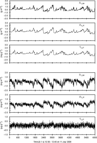
ρ _{v_op} was positively correlated with the fluctuations of vertical wind velocity and sonic temperature. The maximum amplitude of ρ _{v_op} was approximately 1.6 g m⁻³. ρ _{v_cl} had almost the same amplitude as ρ _{v_op} while the fluctuation of ρ _{v_cl} in the high-frequency range attenuated in the sampling tube. ρ _{c_op} showed negative fluctuation with a maximum amplitude of approximately −1.7 mg m⁻³ and was negatively correlated with the vertical wind velocity and sonic temperature fluctuations. The maximum amplitude of ρ _{c_cl} was smaller (−1.2 mg m⁻³) than that of ρ _{c_op} because of the damped temperature fluctuation due to the WPL correction and attenuation of CO₂ density fluctuation itself. The CO₂ density fluctuations in the high-frequency range in the case of both OPGA and CPGA showed almost identical noise owing to the limiting sensitivity of these analysers to measure the small CO₂ density fluctuation over the ocean.

r _{v_cl} showed a positively skewed fluctuation as well as ρ _{v_cl}. r _{c_cl} showed a positively skewed fluctuation, but ρ _{c_cl} showed a negatively skewed fluctuation. Apparently, the CO₂ density fluctuation showed the contrary behaviour from the CO₂ mixing ratio under the significant influence of air temperature and H₂O density fluctuations. Thus, in the present study, the total CO₂ flux by the OPEC changed sign due to the WPL correction, which is similar to the results given by previous studies (Ohtaki et al., 1989; Kondo and Tsukamoto, 2007).

Many observations over land have shown that there was a difference between the lag times for the CO₂ and H₂O fluctuations measured by the CPGA (Ibrom et al., 2007a). The lag time for the H₂O fluctuation was always longer than that for CO₂ fluctuation, and it can be determined empirically as the lag times with which the vertical wind velocity or air temperature fluctuations had to be shifted against both gas fluctuations. However, our observation did not show significant differences between both lag times (1.0–1.4 s) because a short sampling tube (3.2 m) and a high volume pump (12.0 L min⁻¹) were used for the air sampling. McGillis et al. (2004) suggested that the gyroscopic effect due to the ship motion caused false CO₂ signals with the CPGA technique and caused errors in the CO₂ flux. Miller et al. (2010) suggested that the CPGA is more sensitive to this effect than the OPGA. In this study, ship motion effects did not appear in both gas analysers because the motion cycles and magnitudes for our ship were comparatively slow and small during our cruise as shown in Figs. 3 and 4, respectively.

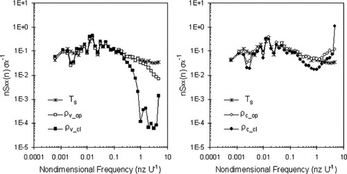
Fig. 4.  A typical example of the normalised power spectra of H₂O (left) and CO₂ (right) densities fluctuations measured by the open-path [open square (left) and open circle (right)] and closed-path [closed square (left) and closed circle (right)] CO₂/H₂O gas analysers; normalised power spectra of the sonic temperature fluctuations (cross) measured by the SAT.

3.2. Spectral analysis

Figure 4 shows a typical example of the normalised power spectra of H₂O (left) and CO₂ (right) densities fluctuations measured by the OPGA and CPGA; that of the sonic temperature (T _s) fluctuation measured by the SAT are also shown. The ordinate on the logarithmic scale is the power spectral density nS _xx (n) normalised by the variance σ ² of each parameter x. The abscissa is the non-dimensional frequency f=nz U ⁻¹ on a logarithmic scale. Here, n is the frequency (Hz) and U is the mean wind speed (m s⁻¹) at the measurement height z (m).

These normalised power spectra had similar frequency structures over a wide frequency range below f=0.19. The normalised power spectrum of ρ _{v_op} followed the −2/3 power law (the inertial subrange) in the wide frequency range (0.05 < f<1.54), similar to T _s. The normalised power spectrum of ρ _{v_cl} also followed the −2/3 power law in the narrower frequency range (0.05 < f<0.19) than that of ρ _{v_op}. Over the frequency range above f=0.19, the normalised power spectrum of ρ _{v_cl} was considerably lower than that of ρ _{v_op} due to the sampling tube attenuation.

The normalised power spectrum of ρ _{c_op} as well as that of ρ _{v_op}, where the white noise appeared, followed the −2/3 power law in the frequency range (0.05 < f<1.54). The normalised power spectrum of ρ _{c_cl} followed the −2/3 power law over the same frequency range (0.05 < f<0.19) as that of ρ _{v_cl}. Moreover, the attenuation of ρ _{c_cl} in the sampling tube appeared in the frequency range of 0.19 < f<0.97, while the white noises of ρ _{c_cl} and ρ _{c_op} appeared over the frequency range above f=0.97.

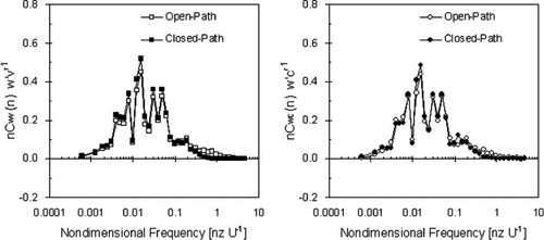
Figure 5 shows a typical example of the normalised cospectra of the above-mentioned parameters and the vertical wind velocity measured by the SAT as a function of the non-dimensional frequency. The ordinate is the cospectrum nC _wx (n), normalised by the flux () of each parameter. Each flux is equivalent to a frequency integral of the cospectrum [C _wx (n)] of each parameter. The cospectra of the H₂O and CO₂ fluxes by the CPEC without the frequency correction are shown in Fig. 5. The shapes of the normalised cospectra of the H₂O and CO₂ fluxes were basically similar over a wide frequency range below f=0.1 as well as that of the normalised cospectrum of the sensible heat flux. This indicates that the assumption of spectral similarity between the CO₂ (or H₂O) flux and sensible heat flux was satisfied, and further, that the bandpass covariance method for the flux correction can be useful. The most dominant frequency range in the cospectra of CO₂ fluxes by the OPEC and CPEC was centred at f=0.016, as were the cospectra of H₂O fluxes. The cospectra of the CO₂ fluxes by both the OPEC and CPEC did not show the effect of white noise, which appeared only in the high-frequency range (Fig. 4). This was because the instrumental white noise of the CO₂ density fluctuation did not correlate with the vertical wind velocity fluctuation. The ratio of the CO₂ (or H₂O) flux loss caused by the sampling tubing attenuation to the flux in the CPEC, corrected by the bandpass covariance method, was 5.0% for CO₂ (2.1–9.1%) and 4.2% for H₂O (3.0–5.8%) fluxes on an average when using the short sampling tube (3.2 m) and high volume pump (12.0 L min⁻¹).

Fig. 5.  A typical example of the normalised cospectra of H₂O (left) and CO₂ (right) fluxes by the OPEC and CPEC as a function of the non-dimensional frequency. Each flux is equivalent to a frequency integral of the cospectrum of each parameter.

3.3. CO₂ fluxes by the OPEC and CPEC techniques

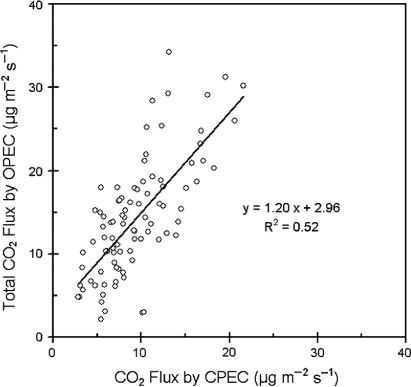
Figure 6 shows the time-series data of the raw CO₂ flux (Raw), the WPL CO₂ correction terms due to air temperature fluctuations (WPL for SHF) and latent heat flux (WPL for LHF), and the total CO₂ flux by the OPEC [F _c(OPEC)], and the CO₂ flux by the CPEC [F _c(CPEC)] during the second run at station A on 10 July 2008. The raw CO₂ flux by the OPEC was an apparent sink and varied from −68.63 to 23.44 µg m⁻² s⁻¹. The WPL correction term for sensible heat flux was always positive and between + 6.63 and + 27.24 µg m⁻² s⁻¹ (the sensible heat flux was between + 3.4 and + 15.0 W m⁻²). The WPL correction term for latent heat flux was between + 19.11 and + 59.61 µg m⁻² s⁻¹ (the latent heat flux was between + 51.4 and + 161.6 W m⁻²). The total CO₂ flux by the OPEC became source (+4.81 to + 13.02 µg m⁻² s⁻¹) after the WPL correction was applied. The CO₂ flux by the CPEC was also source in the range of + 3.10 to + 8.02 µg m⁻² s⁻¹ and somewhat smaller than the total CO₂ flux by the OPEC. Figure 7 shows the point by point comparison of total CO₂ flux by the OPEC and CO₂ flux by the CPEC measured during all special observation times. The total CO₂ flux by the OPEC was on average 20% larger than the CO₂ flux by the CPEC with the offset of 2.96 µg m⁻² s⁻¹; however, its coefficient of determination (R ²) was low (0.52).

Fig. 6.  Time-series data of raw CO₂ flux (Raw, asterisk), the WPL CO₂ correction terms for sensible (WPL for SHF, cross) and latent (WPL for LHF, plus) heat fluxes and total CO₂ flux by the OPEC [F _c(OPEC), open circle], and the CO₂ flux by the CPEC [F _c(CPEC), closed circle] at station A on 10 July 2008.

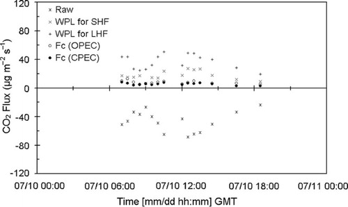
Fig. 7.  Point by point comparison of total CO₂ flux by the OPEC and CO₂ flux by the CPEC measured during all special observation times.

We estimated the bulk CO₂ flux at each station using the mean wind speed and ΔfCO₂ when the flux observation runs were performed for approximately half a day. In this study, the data covered a narrow range of mean wind speed (2.9–5.4 m s⁻¹) and mean ΔfCO₂ (+12.7 to + 41.4 µatm), which drives the source CO₂ flux from the ocean to air at each station. Our results showed that both the CO₂ fluxes directly evaluated by the OPEC and CPEC had the same sign as the estimated bulk CO₂ flux, but were an order of magnitude larger than the bulk CO₂ fluxes (+0.27 to + 1.56 µg m⁻² s⁻¹), as shown in Table 2.

Table 2. Mean values of raw CO₂ flux by the OPEC, WPL CO₂ correction terms for sensible (WPL for SHF) and latent (WPL for LHF) heat fluxes by the OPEC, and total CO₂ flux by the OPEC, the CO₂ flux by the CPEC and bulk CO₂ flux estimated using the gas transfer velocity proposed by Wanninkhof (1992) during the turbulent flux observation runs performed at the four stations

Run	First	Second	Third	Fourth	Fifth	Sixth
Raw flux by OPEC (µg m^−2 s^−1)	−43.85	−46.34	−56.53	−43.89	−60.50	−31.12
WPL for LHF by OPEC (µg m^−2 s^−1)	+33.28	+36.67	+48.40	+42.52	+55.31	+27.65
WPL for SHF by OPEC (µg m^−2 s^−1)	+17.30	+17.34	+22.65	+19.24	+19.19	+11.35
Total flux by OPEC (µg m^−2 s^−1)	+6.73	+7.66	+14.52	+17.87	+13.95	+7.74
Flux by OPEC (µg m^−2 s^−1)	+6.71	+5.46	+8.87	+7.89	+9.78	+8.73
Bulk flux (µg m^−2 s^−1)	+0.27	+0.46	+0.68	+0.54	+1.56	+0.40

There are many possible reasons for the systematic errors in the CO₂ flux by the eddy covariance technique (e.g. tilt correction, block-averaging, de-trending, flow distortion, change in calibration coefficient and cross-sensitivity performance). The tilt correction, block-averaging and de-trending involved low-frequency contributions to the CO₂ flux, but the contributions were relatively small, as shown in Fig. 5. Secondly, the flow distortion is mainly sensitive to the momentum flux because it requires corrections to both the vertical and horizontal velocities, and results in even the momentum flux with an uncertainty of approximately 10–20% (Edson et al., 1998). In the case of the changes in the calibration coefficient and cross-sensitivity performance (Serrano-Ortiz et al., 2007; Prytherch et al., 2010), we made special efforts such as cleaning the OPGA optical windows to avoid contamination by salt particles and raindrops before the special times of turbulent flux observations analysed in this article. In the 1980s discussions, the traditional mismatch between the bulk CO₂ flux by the mass balance technique and the CO₂ flux by the eddy covariance technique was ascribed to the different time and space scales. On the other hand, we believed that this 1980s mismatch was the main cause of the uninvestigated sea salt contamination of the optical window of OPGA. Nevertheless, our results have shown that there is a mismatch between the bulk CO₂ flux and the CO₂ flux by the CPEC in addition to the total CO₂ flux by the OPEC, which were carefully taken care to this contamination like our previous comparison study (Kondo and Tsukamoto, 2007). However, the mismatch in this study is absolutely smaller than the previous 1980s one.

McGillis et al. (2001) and Miller et al. (2010) suggested that the CO₂ flux over oceans be measured by the CPEC in order to eliminate a major source of uncertainty, i.e. the WPL correction. In this study, the WPL correction had significant effects and changed the sign of the CO₂ flux by the OPEC; this was the case in a previous study as well (Kondo and Tsukamoto, 2007). This correction caused a somewhat random error between the CO₂ fluxes by the OPEC with WPL correction and the CPEC without WPL correction; however, it did not cause a systematic error, as shown in Fig. 6. In addition, it has been proved that the theory of WPL correction is not contradictory from previous arguments (Massman and Tuovinen, 2006; Leuning, 2007).

The frequency correction has been identified to be crucial in the processing, especially for the evaluation of small CO₂ fluxes over the ocean by the CPEC. This correction for flux losses depends on the measurement height, wind speed and airflow rates (pump volume) and the dimensions (length and size) of the sampling tube used to sample the air for the CPEC (Leuning and Moncrieff, 1990). Our results have shown that its relatively smaller contribution was 5.0% for CO₂ and 4.2% for H₂O over the ocean if our closed-path system comprised the minimum sampling tube length and the higher volume pump. Significant frequency response correction was required because the CO₂ flux loss contributions are likely to increase when using longer sampling tubes as the previous closed-path measurements over the ocean.

The air–sea bulk CO₂ flux can be estimated by the in situ measured parameters of the sea–air CO₂ fugacity difference, the air and sea surface water temperatures, salinity and wind speed as empirical function of the gas transfer velocity. In this study, each precision of these parameters did not fill the gap between the CO₂ flux by the eddy covariance technique and the bulk CO₂ flux. The primary cause of uncertainties when calculating the bulk CO₂ flux is the uncertain gas transfer velocity. The parameterisation of the CO₂ gas transfer velocity that is itself plotted against the wind speed alone is still problematic. The gas transfer velocity is influenced by a number of processes, but the wind speed has been shown to be the variable that explains the variations in the global gas flux from a practical standpoint. However, such parameterisation is too simplistic, and the scatter of each plot is extremely large over a wide wind speed range. Furthermore, the existing estimations of the gas transfer velocity under the low wind speed (especially, <4 m s⁻¹) conditions, such as the conditions in this study, are insufficient. Recently, Sarma et al. (2010) proposed a novel mass balance technique using stable oxygen isotopes for the direct estimation of the gas transfer velocity and showed that the gas transfer velocity at low wind speeds was higher than the wind speed parameterised estimates based on previous tracers. From comparison of the CO₂ fluxes by the eddy covariance technique during this cruise, we believe the bulk CO₂ flux estimated using this parameterised gas transfer velocity is considerably smaller than that estimated in previous comparison studies. The CO₂ flux by the eddy covariance technique is within the scatter of bulk CO₂ flux involved in the gas transfer velocity estimated by the mass balance technique, although significant differences between the results for both fluxes have been noted.

4. Conclusion

Direct measurements of trace gas fluxes by the eddy covariance technique over coastal seas and open oceans can potentially improve our understanding of the air–sea gas flux caused by various physical and chemical processes, and consequently, improve the precision of the estimated bulk trace gas flux. In this study, we have focused on directly comparing the CO₂ fluxes by OPEC and CPEC over the equatorial Pacific Ocean. Previous studies over oceans deduced a discrepancy between the CO₂ fluxes by both techniques via the bulk CO₂ flux estimated by the mass balance technique. Our primary results, obtained during the special time for the turbulent flux observations with the cleaning of OPGA optical window to avoid contamination by salt particles and raindrops, are summarised as follows.

The sign of the CO₂ flux by the OPEC changed from sink to source due to the significant WPL correction, as in the previous study. The apparent CO₂ density or net mixing ratio fluctuation can be measured by the CPGA with a short sampling tube and high volume air pump. The underestimation of the CO₂ flux in the high frequencies, which is caused by the attenuation of the CO₂ fluctuation in the sampling tube, is approximately 5.0% and can be fully corrected by the bandpass covariance method. Our results over the equatorial Pacific Ocean show a good agreement between the CO₂ fluxes by the OPEC and CPEC, and they are larger than the bulk CO₂ flux estimated using the gas transfer velocity, which was evaluated by mass balance technique.

5. Acknowledgements

We wish to express our heartfelt gratitude to all the crew members of the R/V MIRAI led by Captain Ishioka and Chief Officer Inoue. We are deeply indebted to the staff of JAMSTEC, Marine Work Japan, Ltd. (MWJ), and Global Ocean Development Inc. (GODI). Dr Murata and Dr Yoneyama of JAMSTEC are acknowledged for their invaluable assistance in obtaining the fCO₂, SOAR and SMET data. Special thanks are given to Dr Kashino of JAMSTEC for their arrangements. This work was partially supported by funds from the Grant-in-Aid for Scientific Research in Priority Areas (Grant No. 18067010) of the Ministry of Education, Culture, Sports, Science and Technology (MEXT), Japan. This research is a contribution to the Surface Ocean Lower Atmosphere Study (SOLAS) Core Project of the International Geosphere-Biosphere Programme (IGBP).

References

- Edson J. B, Hinton A. A, Prada K. E, Hare J. E, Fairall C. W. Direct covariance flux estimates from mobile platforms at sea. J. Atmos. Ocean. Technol. 1998; 15: 547–562.
- Grelle A, Lindroth A. Eddy-correlation system for long-term monitoring of fluxes of heat, water vapor and CO2. Glob. Change Biol. 1996; 2: 297–307.
- Hignett P. Corrections to temperature measurements with a sonic anemometer. Boundary-Layer Meteorol. 1992; 61: 175–187.
- Högström U, Bergström H, Smedman A.-S, Halldin S, Lindroth A. Turbulent exchange above a pine forest, I: fluxes and gradients. Boundary-Layer Meteorol. 1989; 49: 197–217.
- Ibrom A, Dellwik E, Jensen N. O, Flyvbjerg H, Pilegaard K. Strong low-pass filtering effects on water vapour flux measurements with closed-path eddy correlation systems. Agric. For. Meteorol. 2007a; 147: 140–156.
- Ibrom A, Dellwik E, Larsen S. E, Pilegaard K. On the use of the Webb–Pearman–Leuning theory for closed-path eddy correlation measurements. Tellus. 2007b; 59B: 937–946.
- Jacobs C. M. J, Kohsiek W, Oost W. A. Air-sea fluxes and transfer velocity of CO2 over the North Sea: results from ASGAMAGE. Tellus. 1999; 51B: 629–641.
- Jones E. P, Smith S. D. A first measurement of sea-air CO2 flux by eddy correlation. J. Geophys. Res. 1977; 82: 5990–5992.
- Kondo F, Tsukamoto O. Air-sea CO2 flux by eddy covariance technique in the equatorial Indian Ocean. 2007; 63: 449–456.
- Lee X, Black A, Novak M. D. Comparison of flux measurements with open- and closed-path gas analyzers above an agricultural field and a forest floor. J. Oceanogr. 1994; 67: 195–202.
- Lenschow D. H, Raupach M. R. The attenuation of fluctuations in scalar concentration through sampling tubes. Boundary-Layer Meteorol. 1991; 96D: 15259–15268.
- Leuning R. The correct form of the Webb, Pearman and Leuning equation for eddy fluxes of trace gases in steady and non-steady state, horizontally homogeneous flows. J. Geophys. Res. 2007; 123: 263–267.
- Leuning R, King K. M. Comparison of eddy-covariance measurements of CO2 fluxes by open- and closed-path CO2 analysers. Boundary-Layer Meteorol. 1992; 59: 297–311.
- Leuning R, Moncrieff J. Eddy-covariance CO2 flux measurements using open- and close-path CO2 analysers: corrections for analyzer water vapour sensitivity and damping of fluctuations in air sampling tubes. Boundary-Layer Meteorol. 1990; 53: 63–76.
- Liss, P. S and Merlivat, L. 1986. Air-sea gas exchange rates: introduction and synthesis. In: The role of air-sea exchange in geochemical cycles. (eds. P.Buat-Manard and D.Reidel). Norwell: MA, pp. 113–127.
- Massman W. J, Tuovinen J.-P. An analysis and implications of alternative methods of deriving the density (WPL) terms for eddy covariance flux measurements. 2006; 121: 221–227.
- McGillis W. R, Edson J. B, Hare J. E, Fairall C. W. Direct covariance air-sea CO2 fluxes. Boundary-Layer Meteorol. 2001; 106C: 16729–16745.
- McGillis, W. R, Edson, J. B, Zappa, C. J, Ware, J. D, McKenna, S. P. and co-authors. 2004. Air-sea CO2 fluxes in the equatorial pacific. J. Geophys. Res. 109: C08S02. 10.3402/tellusb.v64i0.17511.
- McMillen R. T. An eddy correlation technique with extended applicability non-simple terrain. J Geophys. Res. 1988; 43: 231–245.
- Miller, S. D, Marandino, C and Saltzman, E. S. 2010. Ship-based measurement of air-sea CO2 exchange by eddy covariance. Boundary-Layer Meteorol. 115: D02304. 10.3402/tellusb.v64i0.17511.
- Murata A, Takizawa T. Summertime CO2 sinks in shelf and slope waters of the western Arctic Ocean. J Geophys. Res. 2003; 23: 753–776.
- Ohtaki E, Tsukamoto O, Iwatani Y, Mitsuta Y. Measurements of the carbon dioxide flux over the ocean. Cont. Shelf Res. 1989; 67: 541–554.
- Ono, K, Hirata, R, Mano, M, Miyata, A, Saigusa, N. and co-authors. 2007. Systematic differences in CO2 fluxes measured by open- and closed-path eddy covariance systems: influence of air density fluctuations resulting from temperature and water vapor transfer. J. Meteorol. Soc. Japan. 63: 139–155.
- Prytherch, J, Yelland, M. J, Pascal, R. W, Moat, B. I, Skjelvan, I. and co-authors. 2010. Direct measurements of the CO2 flux over the ocean: development of a novel method. J. Agric. Meteorol. 37: L03607. 10.3402/tellusb.v64i0.17511.
- Sahlée E, Drennan W. M. Measurements of damping of temperature fluctuations in a tube. Geophys. Res. Lett. 2009; 132: 339–348.
- Sarma V. V. S. S, Abe O, Honda M, Saino T. Estimating of gas transfer velocity using triple isotopes of dissolved oxygen. Boundary-Layer Meteorol. 2010; 66: 505–512.
- Serrano-Ortiz P, Kowalski A. S, Domingo F, Ruiz B, Alados-Arboledas L. Consequences of uncertainties in CO2 density for estimating net ecosystem CO2 exchange by open-path eddy covariance. J. Oceanogr. 2008; 126: 209–218.
- Serrano-Oriz P, Kowalski A. S, Domingo F, Ruiz B, Alados-Arboledas L. Consequences of uncertainties in CO2 density for estimating net ecosystem CO2 exchange by open-path eddy covariance. Boundary-Layer Meteorol. 2007; 126: 209–218.
- Smith S. D, Jones E. P. Evidence for wind-pumping of air-sea gas exchange based on direct measurements of CO2 fluxes. J. Geophys. Res. 1985; 90C: 869–875.
- Suyker A. E, Verma S. B. Eddy correlation measurements of CO2 flux using a closed-path sensor: theory and field test against an open-path sensor. Boundary-Layer Meteorol. 1993; 64: 391–407.
- Takahashi, S, Kondo, F, Tsukamoto, O, Ito, Y, Hirayama, S. and co-authors. 2005. On-board automated eddy flux measurement system over open ocean. SOLA. 1: 37–40.
- Verma, S. B, Ullman, F. G, Billesbach, D, Clement, R. J.,Kim, J. and co-authors. 1992. Eddy correlation measurements of methane flux in a northern peatland ecosystem. Boundary-Layer Meteorol. 58: 289–304.
- Wanninkhof R. Relationship between wind speed and gas exchange over the ocean. Boundary-Layer Meteorol. 1992; 97C: 7373–7382.
- Watanabe T, Yamanoi K, Yasuda Y. Testing of the bandpass eddy covariance method for a long-term measurement of water vapour flux over a forest. Q. J. R. Meteorol. Soc. 2000; 96: 473–491.
- Webb E. K, Pearman G. I, Leuning R. Correlation of flux measurement for density effects due to heat and water vapour transfer. Boundary-Layer Meteorol. 1980; 106: 85–100.
- Weiss, R. F. 1974. Carbon dioxide in water and seawater: the solubility of a non-ideal gas. Mar. Chem. 2: 203–215, 10.3402/tellusb.v64i0.17511.
- Yasuda Y, Watanabe T. Comparative measurements of CO2 flux over a forest using closed-path and open-path CO2 analysers. J. Geophys. Res. 2001; 100: 191–208.