Annual variation of CH₄ emissions from the middle taiga in West Siberian Lowland (2005–2009): a case of high CH₄ flux and precipitation rate in the summer of 2007

ABSTRACT

We described continuous measurements of CH₄ and CO₂ concentration obtained at two sites placed in the middle taiga, Karasevoe (KRS) and Demyanskoe (DEM), in West Siberian Lowland (WSL) from 2005 to 2009. Although both CH₄ and CO₂ accumulation (ΔCH₄ and ΔCO₂) during night-time at KRS in June and July 2007 showed an anomalously high concentration, higher ratios of ΔCH₄/ΔCO₂ compared with those in other years indicated that a considerably higher CH₄ flux occurred relative to the CO₂ flux. The daily CH₄ flux calculated with the ratio of ΔCH₄/ΔCO₂ and terrestrial biosphere CO₂ flux from an ecosystem model showed a maximum in July at the both sites. Although anomalously high flux was observed in June and July 2007 at KRS, only a small flux variation was observed at DEM. The high regional CH₄ flux in June and July 2007 at KRS was reproduced using a process-based ecosystem model, Vegetation Integrative Simulator for Trace gases (VISIT), in response to high water table depth caused by the anomalously high precipitation during the summer of 2007.

• methane
• Siberia
• taiga
• West Siberian Lowland
• tower observation

1. Introduction

Atmospheric CH₄ is the second most important anthropogenic greenhouse gas after CO₂ because of its influence on the Earth's radiation budget through infrared absorption and its role in the photochemistry of the atmosphere. Its concentration in the troposphere is principally determined by a balance between surface emission and destruction by hydroxyl (OH) radicals. Anthropogenic CH₄ emission sources include fossil fuel combustion, rice agriculture, livestock, landfill, waste treatment and biomass burning, while major natural sources include wetlands, termites and the ocean (IPCC, 2007). The anthropogenic emissions following the industrial revolution in the 1850s produced an exponential increase in the global CH₄ content followed by a period of relatively stable concentration from 1999 to 2006 (Dlugokencky et al., 2003; Rigby et al., 2008). The period of stable concentration has been partly attributed to a decrease in CH₄ emissions of ˜10 Tg from the region North of 50°N (the former Soviet Union) from 1990 to 1995 (Dlugokencky et al., 2003). This is consistent with the results of inverse calculations, which have attributed the stabilisation of atmospheric CH₄ to a steady decrease in anthropogenic CH₄ emissions between 1990 and 1999 (Bousquet et al., 2006). Bousquet et al. (2006) also showed that anthropogenic CH₄ emissions increased after 1999, but the CH₄ concentration in the atmosphere remained relatively constant because of a coincidental decrease in wetland emissions for several years after 1999. Rigby et al. (2008) reported that the CH₄ concentration began to increase again at the beginning of 2007 and speculated that Siberian wetlands were the most likely source because of an anomalously high annual mean temperature over Siberia (˜4°C above the 1961–1990 base climatology). Dlugokencky et al. (2009) examined the observational data obtained from the background sites operated by the National Oceanic and Atmospheric Administration (NOAA) and reported that the increase in the atmospheric CH₄ concentration in the early 2007 persisted until 2008. They suggested that the very warm temperatures at polar northern latitudes during 2007 likely enhanced the CH₄ emissions from the northern wetlands. Despite the importance of CH₄ emissions from the Siberian wetlands to the globally elevated CH₄ concentration since 2007, substantial uncertainties remain in estimating the CH₄ fluxes and responses to climate change. This is mainly due to the sparseness of in situ observation during this period (˜2007) in Siberia. For example, Kozlova et al. (2008) presented the first results of continuous in situ CH₄ concentration measured at the Zotino Tall Tower Observatory (ZOTTO; 60°48′N, 89°21′E) in the boreal forest of central Siberia, but the study showed measurements only from November to December, 2006. Recently, a 1-year time series of CH₄ concentration (May 2009–April 2010) at ZOTTO was published by Winderlich et al. (2010). The CH₄ concentration had no seasonal variation but showed a distinct diurnal cycle during the summer (July 2009). In order to increase the spatio-temporal coverage, we have been operating, since 2004, an expanded network of towers (JR-STATION: Japan-Russia Siberian Tall Tower Inland Observation Network) located in taiga, steppe and wetland biomes of Siberia. Sasakawa et al. (2010) conducted some analysis of the data from the network and found that the number of elevated CH₄ concentration events in the summer was greatest in 2007 when temperature and precipitation rates were highest for 2004–2008 monitoring period over West Siberia. They suggested that the elevated CH₄ concentration events observed in 2007 could be attributed mainly to the enhanced emissions from wetlands.

In this study, we estimated hourly CH₄ flux from the middle taiga in WSL utilising the observed CH₄ and CO₂ concentration from the JR-STATION monitoring program and CO₂ flux from an ecosystem model. Five years (2005–2009) of continuous measurements have made it possible to characterise the seasonal and annual variations of the CH₄ flux. A process-based ecosystem model, Vegetation Integrative Simulator for Trace gases (VISIT) (Inatomi et al., 2010; Ito, 2010), was used to estimate the CH₄ fluxes responding to weather and biological conditions.

2. Method

2.1. Site description and measurement system

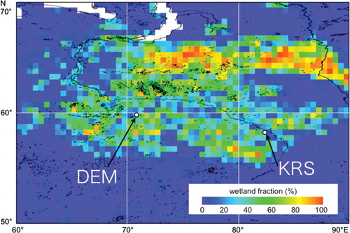
In this study we focused on two sites from the JR-STATION program; Karasevoe (KRS) tower (58°15′N, 82°25′E) and Demyanskoe (DEM) tower (59°47′N, 70°52′E) (Fig. 1). Both towers are placed in the middle taiga and surrounded by bogs. No large city exists in 200 km around both towers; thus, CH₄ emitted from wetlands is the major contributor to CH₄ variation particularly during summer (Sasakawa et al., 2010). We installed a freight container equipped with gas analysers and a data logger at the base of each tower. Atmospheric air was sampled at two levels on the towers; 35 m and 67 m at KRS, and 45 m and 63 m at DEM. Sampled air was dried and then introduced into a non-dispersive infrared analyser (model LI-820, LI-COR, USA) and an originally developed CH₄ semiconductor sensor (Suto and Inoue, 2010). The air-sampling flow path was rotated every 20 min; that is, the high inlet was sampled on the hour at hh:00, the low inlet 20 min later at hh:20, and a reference gas 40 min later at hh:40 (i.e. 20 min after the low inlet sampling). For each 20-min sampling period, air was pumped continuously through the sample line, a stainless tube containing chemical desiccant (magnesium perchlorate), NDIR cell and CH₄ sensor for the first 17 min (flushing); for the following 3 min, the data produced by the sensors were averaged and taken as the representative data for the applicable 1-h period. Thus, both the data from the high and low inlets were shown as the data at hh:30. Measurement precision was ±0.3 ppm and ±3 ppb for CO₂ and CH₄, respectively (Sasakawa et al., 2010).

Fig. 1.  Wetland distribution map based on GLWD (Lehner and Döll, 2004) used in VISIT model. Grid colour indicates the wetland fraction for each grid. For example, 50% (green) means that half of the surface in the grid is regarded as wetland. KRS and DEM denote the tower position at Karasevoe (58°15′N, 82°25′E) and Demyanskoe (59°47′N, 70°52′E), respectively.

2.2. Methane flux estimation

The degree of nocturnal accumulation in CO₂ and CH₄ concentrations generally depends on the regional surface fluxes and atmospheric stability. We then estimated the daily CH₄ flux from terrestrial biosphere CO₂ flux normalised with the observed CH₄ and CO₂ accumulation on a certain day:1

Here, we defined gas accumulation (ΔCO₂ and ΔCH₄) as the measured concentration difference between the concentration at 21:30 Local Standard Time (LST) and the elevated concentration at early next morning (4:30 LST). The ratio of ΔCH₄/ΔCO₂ indicated only the relative strength of the flux of CH₄ and CO₂. The CH₄ flux calculated from eq. (1) reflected averaged emissions around each tower. For three-hourly CO₂ fluxes were generated from the monthly Net Ecosystem Production (NEP) fluxes produced by the Carnegie-Ames-Stanford Approach (CASA) ecosystem model (Randerson et al., 1997) on a 1°×1° grid using a procedure similar to that of Olsen and Randerson (2004). We used the data from the JMA Climate Data Assimilation System (JCDAS; Onogi et al., 2007) as the source of meteorological fields. First, the three-hourly downward short-wave radiation was calculated by fitting the six-hourly JCDAS data to a theoretical clear-sky solar radiation function. Then, the three-hourly Gross Primary Production (GPP) within each month was estimated by distributing the monthly GPP [Net Primary Production (NPP)×2] in accordance with the radiation data. Thereafter, the monthly respiration (R _e) was distributed within each month according to:2

where Q ₁₀ was set at 1.5 (Olsen and Randerson, 2004) and T was obtained from the 2-m JCDAS temperature. Then, R _e,o was adjusted so that the monthly NEP (GPP – R _e) approached the same values as the original CASA NEP data, with zero mean annual biospheric flux at every grid point. The three-hourly CASA CO₂ fluxes showed clear diurnal variation with negative and positive values during the daytime and the night-time, respectively, in the summer (not shown). We used the average of three midnight data [21:30 LST (day x), 0:30 LST (day x+1) and 3:30 (day x+1)] over the targeted area (±3° latitude, ±1° longitude) around the towers (KRS and DEM) as .

Although most of the results from the low inlet indicated the same as those from the high inlet, we showed those from the high inlet to remove occasional local influence. It should be noted that the calculated CH₄ flux turned out to be the minimum estimated value because some wetlands showed higher CH₄ flux during the daytime than during the night-time (e.g. Hargreaves and Fowler, 1998; Long et al., 2010). However, the elevated CH₄ flux during the daytime was not always observed (Long et al., 2010), and it has been shown that, at some wetlands, a diurnal cycle of CH₄ flux is not observed (Werner et al., 2003; Rinne et al., 2007).

2.3. Ecosystem model

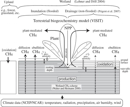
Monthly CH₄ fluxes from wetlands were estimated using the VISIT model (Inatomi et al., 2010; Ito, 2010) to evaluate the variation of gas fluxes responding to weather and biological conditions. Figure 2 shows a schematic diagram of the CH₄ exchange processes employed in VISIT. The model consists of carbon, nitrogen and water cycle subschemes, each of which is composed of several functional compartments such as leaves, stems, roots, dead biomass and organic soil. Plant photosynthetic CO₂ uptake, allocation, biomass growth and mortality are simulated in the carbon cycle as part of an ecophysiological process (Ito and Oikawa, 2002). Wetland CH₄ flux is simulated using a semi-mechanistic scheme (Walter and Heimann, 2000), in which three processes of CH₄ flux emission are considered: physical diffusion, plant-mediated transportation and ebullition. The physical diffusion rate depends on the CH₄ concentration gradient between the surface and soil air, which is affected by the CH₄ production and oxidation within the soil. In the soil, the CH₄ production rate is determined by microbial activity and substrate supply from plants, producing sensitivity to temperature variability that leads clearly to seasonal cycle in the CH₄ emission (Le Mer and Roger, 2001). Spatial heterogeneity in diffusivity through soil pore spaces is determined on the basis of sand/clay composition data (Hall et al., 2006) and water table depth. The plant-mediated transport of CH₄ is dependent on the plant growing stage determined by the cumulative temperature and biome-specific rooting depth (typically, 20 cm for wetlands). The ebullition flux occurs only when the CH₄ concentration exceeds 500 µmol L⁻¹ (Walter and Heimann, 2000). It should be noted that, due to the lack of site-specific ecological measurements, several variables in the model are assigned typical values reflecting the general characteristics of the northern wetlands. This introduced a potential uncertainty in our study, which will be discussed later.

Fig. 2.  A schematic diagram of the CH₄ exchange scheme used in this study.

Wetland distribution is determined on a 0.5°×0.5° grid based on Global Lakes and Wetlands Database (GLWD, Lehner and Döll, 2004) (Fig. 1). A distribution of natural vegetation type including both uplands and wetlands is derived from the global data-set (Olson et al., 1983; Ramankutty and Foley, 1999). For performing broad-scale simulations, wetland soils are stratified into 20 layers of 5 cm thickness each. To include the spatial heterogeneity of wetlands, CH₄ fluxes are separately estimated for flooded (i.e. inundation) and non-flooded fractions of the ground surface, each of which has different water table depths. Thus, the total CH₄ emission (E) for each grid cell is obtained as:3

where w represents the wetland fraction in each grid cell, and f and E denote the land fraction and CH₄ exchange flux of inundation and drainage parts (subscripts), respectively. Monthly averaged inundation fraction (f _inund) is derived from a passive microwave Special Sensor Microwave/Imager (SSM/I) observation for 1993–2000 (e.g. Prigent et al., 2007). Because we estimated the inundation fraction on the basis of seasonal variation for each grid cell in this study, snow cover and extensive flooding after snow melting could in some cases affect the baseline. To avoid these apparent variations (e.g. too much severe drying after a spring flood) during the growing period (May–August), we decided to use the averaged inundation fraction derived from the SSM/I observation during the period. The baseline water table depths of the inundated and drained wetland surfaces were assumed to be 0 and –25 cm, respectively, based on a simulation at West Siberian wetlands (Bohn et al., 2007). At layers lower than the water table, the CH₄ production is estimated in the model as a function of temperature and plant carbon supply that is obtained from the vegetation production scheme. The simulated CH₄ flux reflected the minimum estimated value in our study since the assumed water table depth for a drained surface (–25 cm) was the lowest case scenario; higher water table depths could produce higher CH₄ fluxes due to the resulting reduction in the oxidation zone (Fig. 2).

We also evaluated the influence of precipitation rate on the CH₄ emission from wetlands. Inter-annual variability in the water table depth was estimated from the cumulative precipitation anomaly at each model grid as deviation from the 2001 to 2009 mean, which was obtained from the NCEP/NCAR reanalysis data (Kalnay et al., 1996). To assess the possible range of estimation, a high (+1 mm water table depth/ + 1 mm precipitation anomaly) and a low (similarly, +0.2 mm/ + 1 mm) response cases were examined.

3. Results and discussions

3.1. Summer diurnal variation in CO₂ and CH₄ concentration

Both the CO₂ and CH₄ concentration at KRS and DEM showed clear diurnal variation during the summer (Fig. 3). Diurnal amplitude exhibited maximum in July for both CO₂ (>15 ppm) and CH₄ (>100 ppb). If the wind blows from different specific directions between day and night (e.g. a northerly in the daytime and a southerly in the night-time), the observed diurnal variation could be caused by the footprint. However, there was no dominant wind direction and no particular difference in the wind direction between day and night, allowing for an assumption of relatively homogeneously distributed sources of CO₂ and CH₄ over the tower footprint; that is, sources of these gases were essentially co-located. The diurnal cycle of CO₂ is basically controlled by plant photosynthesis and respiration during the daytime and respiration during the night-time. The lower atmosphere night-time CO₂ accumulation is amplified by the development of a stable nocturnal boundary layer (NBL). For CH₄, the emission from wetlands is relatively constant during the day (Werner et al., 2003; Rinne et al., 2007; Long et al., 2010) or higher during the daytime (Hargreaves and Fowler, 1998; Long et al., 2010) in the summer, the development of NBL and the lowering of the mixed layer (ML) height are the major factors contributing to the night-time buildup of its concentration, and thus causing the observed diurnal variation. It has been observed that the ML height over Siberia is clearly dependent on the season, varying from 200–600 m in the winter to as much as 2800 m in the summer (Lloyd et al., 2002). Diurnally, it begins to develop in the morning and the height continues to increase during the daytime. This causes a decrease in the CH₄ concentration due to increased volume of dilution and the mixing with the free tropospheric air with a lower CH₄ concentration. After sunset, the convective ML collapses, followed by CH₄ accumulation. In our study, the timing of the diurnal maximum in CO₂ concentration (4:30–6:30 LST) was observed to occur earlier than that in CH₄ concentration (5:30–8:30 LST) (Fig. 3). This slight lag in the peaking of the concentration of CO₂ and CH₄ was caused mainly by the fact that photosynthesis due to solar radiation started before the development of convective ML.

Fig. 3.  Mean diurnal variation of CO₂ and CH₄ concentrations during summer (June, July and August) at KRS and DEM. The data from high inlet were annually averaged. Vertical dotted lines indicate the mean time of sunrise and sunset. Every 12 h, all three measurements for the hour were of standard gases; thus, there are no data at 8:30 LST and 20:30 LST.

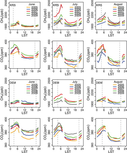
Figure 3 does not indicate any clear long-term increasing trend in the night-time CO₂ concentration while the daytime CO₂ concentration from 2005 to 2009 shows a general increasing trend. This is because the degree of nocturnal accumulation strongly depends on the daily regional surface flux and weather condition (atmospheric stability), while the daytime concentrations generally represent values from a wider region due to the well-mixed condition of the atmosphere. In our study, the daytime and night-time CH₄ concentrations did not show any discernable increasing trend, but did exhibit positive anomaly in July 2007 both at KRS and DEM.

3.2. Estimation of CH₄ emissions

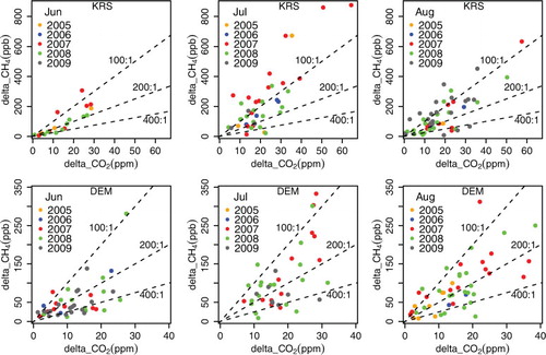
Scatter plots of ΔCH₄ versus ΔCO₂ at our sites show that the CH₄ flux was generally greater than 1/400 CO₂ flux (Fig. 4). It is also noted in Fig. 4 that the ratios of ΔCH₄/ΔCO₂ in July 2007 at KRS show a general increase in the CH₄ flux of more than four times compared to the CO₂ flux (ratio values≧4/400 = 1/100). This corresponded to the particularly hot and wet weather in West Siberia during the summer of 2007, likely creating favourable conditions for increased CH₄ emissions from bogs. Remarkable high ratios were also seen in August 2009 at KRS when the precipitation rate was anomalously high during summer (see Section 3.3). No obvious seasonality was found in the ratio of ΔCH₄/ΔCO₂, although summer maximum was observed in July at KRS.

Fig. 4.  Relationship between ΔCO₂ and ΔCH₄ during summer at KRS (upper panels) and DEM (lower panels). ΔCO₂ and ΔCH₄ are defined as the measured concentration difference between the concentration at 21:30 LST and the accumulated concentration in the early morning the next day at 4:30 LST. Dotted lines indicate expected relationship from environment in CO₂-flux:CH₄-flux = 100:1, 200:1 and 400:1.

Calculated CH₄ flux with eq. (1) displayed a clear seasonal cycle, with maximum in July (Fig. 5), corresponding to the clear increase in daytime CH₄ concentrations as reported by Sasakawa et al. (2010). There was also considerable monthly variability in CH₄ flux, particularly during summer. The seasonality was produced mainly because the nocturnal CASA CO₂ fluxes due to respiration showed a maximum in June and July (˜6 µmol m⁻² s⁻¹) and a minimum in winter (<1 µmol m⁻² s⁻¹).

Fig. 5.  Box-and-whisker diagrams of daily CH₄ flux calculated with nocturnal CO₂ and CH₄ accumulation over an area (±3° latitude, ±1° longitude) around (a) KRS and (b) DEM. The diagrams are defined as follows: the median is the thick line in the box; the bottom and top of the box are the lower and upper quartiles, respectively; the whiskers extend to the most extreme data point which is no more than one time the interquartile range from the box; individual outliers are shown as open circles outside the whiskers. Horizontal grey lines indicate regional means of fluxes from the wetlands (bogs, swamps and tundra) in the GISS model. Closed diamonds denote monthly CH₄ flux simulated with VISIT model. Open (grey) diamonds denote monthly CH₄ flux of high (low) response case for precipitation anomaly. The bottom figures show the number of calculated day for each month and year. It depends mostly on the number of the obtained data. No winter data are shown since there is almost no diurnal variation during winter (Sasakawa et al., 2010).

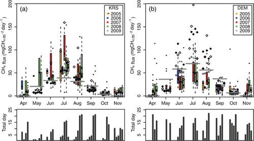
Methane fluxes in June and July 2007 around KRS were noticeably higher than those in other years (Fig. 5a). The longest upper quartile range for July 2005 resulted from (1) very few data obtained during the month and (2) one anomalous datum for the month, which is plotted significantly above the 100:1 ratio line in Fig. 4. Methane fluxes in August 2009 exhibited higher values than those in the previous years. Generally CH₄ fluxes around DEM were lower than those around KRS, and no anomalous high flux in July 2007 appeared (Fig. 5b). It should be noted that the anomaly in CH₄ flux was quite different between the two sites, although both sites were placed in the middle taiga in WSL. The calculated CH₄ fluxes in June, July and August around KRS were higher than the regional mean flux estimates for the wetlands from Goddard Institute for Space Studies (GISS) (Fung et al., 1991; Patra et al., 2009) (Fig. 5a). The GISS data-set applied scaling factors to each individual component as shown in Patra et al. (2009); this flux varies from month to month, but does not change from year to year for the same month. The difference in flux values was possibly due to the relatively coarse resolution of the GISS flux map, which does not resolve many of the small ponds and lakes that are distributed throughout the taiga and extensive bogs surrounding the KRS tower; these small water bodies can act as a significant source of CH₄, particularly during summer (e.g. Repo et al., 2007). Repo et al. (2007) reported that the daily mean emission of CH₄ from small wetland lakes in western Siberia ranged from 1.1 to 120 mg m⁻² d⁻¹, which can contribute to the difference. On the other hand, the GISS data showed higher flux estimates around DEM compared to our calculated values (Fig. 5b), perhaps pointing to an overestimation of CH₄ flux by GISS for wetlands, at least in the regions around DEM.

In situ measurements of CH₄ flux from Siberian wetlands are scarce and limited to short periods. Panikov and Dedysh (2000) reported that the monthly average CH₄ fluxes measured using a static chamber technique at a West Siberian bog near the village of Plotnikovo (56°51′N, 82°58′E) in July and/or August 1993–1997 ranged from 137 to 465 mg m⁻² d⁻¹. Friborg et al. (2003) measured CH₄ flux with eddy correlation technique at the same bog in West Siberia during the summer of 1999; the average CH₄ flux in three campaigns varied from 75 to 222 mg m⁻² d⁻¹. Whereas these in situ measurements displayed emission rates specific to a narrow region, Takeuchi et al. (2003) extrapolated field observations taken in July 1993 and 1994 to an area 400 km×400 km adjacent to Plotnikovo, using land cover classifications derived from NOAA AVHRR and SPOT HRV images; these results were comparable with our calculated regional CH₄ fluxes in this study. Their estimation of regional average CH₄ flux for July 1993 and 1994 was 59.3 mg m⁻² d⁻¹, which fell in the interquartile range for July around the DEM and KRS region, except for July 2007.

3.3. Estimation of CH₄ with VISIT model

We simulated CH₄ emissions from the middle taiga with the VISIT model. The regional mean rates of the simulated CH₄ emission generally reproduced the observed seasonal variations at KRS and DEM, with maximum in July (Fig. 5). The overall regional strength of the CH₄ emission at KRS agreed well with the results of the observation-based calculation with eq. (1), despite the overestimation at DEM. However, annual variation was small and anomalously high CH₄ emission in June and July 2007 at KRS was not reproduced. This might be because observational information on factors (water table, rooting depth, etc.) influencing the calculation of CH₄ emission from forested bogs is quite limited.

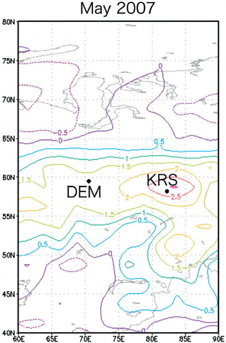
Based on model simulations, Bohn et al. (2007) evaluated the sensitivity of CH₄ emission from a 100 km×100 km region near Plotnikovo to increases in temperature and precipitation. They found that higher temperatures alone did not always increase CH₄ emissions from wetlands but higher precipitation alone raised water tables and expanded the saturated area, resulting in a net increase in the CH₄ emissions. Monthly mean precipitation rate for the area around the KRS region obtained from the Global Precipitation Climatology Project (GPCP) version 2.1 combined precipitation data set (Adler et al., 2003) showed high precipitation rates of 4.4 and 3.6 mm d⁻¹ in May and June 2007, respectively. These values were 2.7 and 1.6 mm d⁻¹ higher than the respective monthly averages for the 1979–1998 climatological period and represented the highest values during the period of our study. These precipitation rates of about two times the climatological mean (Fig. 6) probably elevated the water table in the KRS region, leading to an increase in the CH₄ emissions from the surrounding wetlands. In June and July 2009, the precipitation anomalies were also high (1.3 and 1.0 mm d⁻¹ above the climatology) in the KRS region and most likely resulted in an elevated CH₄ flux in August (Fig. 5a). The slight time lag between the time of high precipitation rate and the time of increased CH₄ emission was likely due to the poor drainage in the West Siberian wetlands (relatively flat terrain) and low evapotranspiration rate.

Fig. 6.  Anomaly of precipitation rate (mm d⁻¹) in May 2007 relative to the monthly average of the 1979–1998 period obtained from GPCP version 2.1 combined precipitation data set (Adler et al., 2003).

In order to verify the model sensitivity of CH₄ flux to water table depth, we modified the VISIT model so that the dimension of the water table depth was assumed to expand proportionally to the monthly precipitation anomaly rates (see Section 2.3). As shown in Fig. 2, the elevated water table depth increases the CH₄ production zone and decreases its oxidation zone in the model, leading to an increase in the CH₄ flux from the wetlands. The simulated regional mean CH₄ emission rates showed a maximum in July. The extremely high regional CH₄ emission in June and July 2007 at KRS was reproduced as 72 (37) and 159 (83) mg CH₄ m⁻² d⁻¹ in the high (low) response case (Fig. 5a), in response to high water table depth caused by the anomalously high precipitation during the summer of that year. These results support the hypothesis that the high precipitation rate in the summer of 2007 accounted for the high CH₄ emissions from regions around KRS.

Integrated CH₄ emissions in a high (low) response case from the middle taiga around KRS (±3° latitude, ±1° longitude; approximately 7.8×10⁴ km²) resulted in 0.54 (0.39), 0.31 (0.34), 0.94 (0.48), 0.44 (0.36) and 0.41 (0.39) Tg CH₄ yr⁻¹ for the years 2005–2009, respectively. Most of the previous studies (e.g. Rigby et al., 2008; Dlugokencky et al., 2009) speculated that the Siberian wetlands were the main source for the CH₄ increase from the beginning of 2007. Although the emission in 2007 around KRS was two to three times greater than those in other years, the anomalous CH₄ emission from the targeted area around KRS by itself was not enough to explain all the recently observed variability in the global CH₄ concentration growth. In addition, no anomalous CH₄ emission was observed around DEM.

4. Conclusions

We calculated the daily CH₄ flux with measured concentrations of CH₄ and CO₂, and the terrestrial biosphere CO₂ flux from the CASA ecosystem model. The calculated CH₄ flux from the middle taiga around KRS and DEM in WSL from 2005 to 2009 showed a maximum in July. Although anomalously high flux was observed in June and July 2007 and August 2009 at KRS, only a small variation in the flux at DEM was observed. These results indicated that the variation in CH₄ flux from the Siberian wetlands was not uniform in space and time. The strength of the calculated CH₄ flux could be changed if anomalous weather condition leads to an extreme increase/decrease in CO₂ flux from vegetation respiration, but an assessment of this uncertainty requires a better estimation of CO₂ flux that includes yearly variation.

Using VISIT, the ecosystem model in which the dimension of the flooded area was assumed to expand proportionally with the cumulative anomaly in monthly precipitation rate, we confirmed that the anomalously high CH₄ flux in the summer of 2007 around KRS could have resulted from the high precipitation rate. The shortcomings of our approach stemmed from the fact that the values assigned to the variables (such as water table depth) influencing the CH₄ flux were not based on the site-specific measurements, but on a general ecological characterisation of the region. In order to reduce the uncertainty in our model estimation of the CH₄ flux, we need to constrain the model calculation using actual observational data.

5. Acknowledgements

We would like to thank Sergey Mitin (Institute of Microbiology, Russian Academy of Sciences) for administrative support. We also express our sincere thanks to Yasunori Tohjima (NIES) for providing us with fruitful comments on flux calculation. Kaz Higuchi (York University) is acknowledged for the critical reading of the manuscript and for English language corrections. This research was supported by the Global Environment Research Account for National Institutes of the Ministry of the Environment, Japan, through its funding of the project titled: Estimation of CO₂ and CH₄ Fluxes in Siberia using Tower Observation Network.

References

- Adler, R, Huffman, G, Chang, A, Ferraro, R, Xie, P. and co-authors. 2003. The version-2 global precipitation climatology project (GPCP) monthly precipitation analysis (1979–present). J. Hydrometeor. 4: 1147–1167.
- Bohn, T. J, Lettenmaier, D. P, Sathulur, K, Bowling, L. C, Podest, E. and co-authors. 2007. Methane emissions from western Siberian wetlands: heterogeneity and sensitivity to climate change. Environ. Res. Lett. 2: 10.3402/tellusb.v64i0.17514.
- Bousquet, P, Ciais, P, Miller, J. B, Dlugokencky, E. J, Hauglustaine, D. A. and co-authors. 2006. Contribution of anthropogenic and natural sources to atmospheric methane variability. Nature. 443: 439–443.
- Dlugokencky, E. J, Houweling, S, Bruhwiler, L, Masarie, K. A, Lang, P. M. and co-authors. 2003. Atmospheric methane levels off: temporary pause or a new steady-state?. Geophys. Res. Lett. 30: 10.3402/tellusb.v64i0.17514.
- Dlugokencky, E. J, Bruhwiler, L, White, J. W. C, Emmons, L. K, Novelli, P. C. and co-authors. 2009. Observational constraints on recent increases in the atmospheric CH4 burden. Geophys. Res. Lett. 36: 10.3402/tellusb.v64i0.17514.
- Friborg, T, Soegaard, H, Christensen, T, Lloyd, C and Panikov, N. 2003. Siberian wetlands: where a sink is a source. Geophys. Res. Lett. 30: 10.3402/tellusb.v64i0.17514.
- Fung, I, John, J, Lerner, J, Matthews, E, Prather, M. and co-authors. 1991. Three-dimensional model synthesis of the global methane Cycle. J. Geophys. Res. 96: 13033–13065.
- Hall, F. G, de Colstoun, E. B, Collatz, G. J, Landis, D, Dirmeyer, P. and co-authors. 2006. ISLSCP Initiative II global data sets: surface boundary conditions and atmospheric forcings for land-atmosphere studies. J. Geophys. Res. 111: 10.3402/tellusb.v64i0.17514.
- Hargreaves K, Fowler D. Quantifying the effects of water table and soil temperature on the emission of methane from peat wetland at the field scale. Atmos. Environ. 1998; 32: 3275–3282. 10.3402/tellusb.v64i0.17514.
- Inatomi M, Ito A, Ishijima K, Murayama S. Greenhouse gas budget of a cool-temperate deciduous broad-leaved forest in Japan estimated using a process-based model. Ecosystems. 2010; 13: 472–483. 10.3402/tellusb.v64i0.17514.
- IPCC. 2007. Climate Change 2007: the physical science basis, contribution of working group I. In: The Fourth Assessment, Report of the Intergovernmental Panel on Climate Change. (S.Solomon, D.Qin, M.Manning, Z.Chen, M.Marquis, and co-editors.). New York: Cambridge University Press. 996pp.
- Ito A, Oikawa T. A simulation model of the carbon cycle in land ecosystems (Sim-CYCLE): a description based on dry-matter production theory and plot-scale validation. Ecol. Model. 2002; 151: 143–176. 10.3402/tellusb.v64i0.17514.
- Ito A. Changing ecophysiological processes and carbon budget in East Asian ecosystems under near-future changes in climate: implications for long-term monitoring from a process-based model. J. Plant Res. 2010; 123: 577–588. 10.3402/tellusb.v64i0.17514.
- Kalnay, E, Kanamitsu, M, Kistler, R, Collins, W, Deaven, D. and co-authors. 1996. The NCEP/NCAR 40-year reanalysis project. Bull. Am. Meteor. Soc. 77: 437–471.
- Kozlova, E. A, Manning, A. C, Kisilyakhov, Y, Seifert, T. andHeimann, M. 2008. Seasonal, synoptic, and diurnal-scale variability of biogeochemical trace gases and O2 from a 300-m tall tower in central Siberia. Glob. Biogeochem. Cycles. 22: 10.3402/tellusb.v64i0.17514.
- Le Mer J, Roger P. Production, oxidation, emission and consumption of methane by soils: a review. Eur. J. Soil Biol. 2001; 37: 25–50. 10.3402/tellusb.v64i0.17514.
- Lehner B, Doll P. Development and validation of a global database of lakes, reservoirs and wetlands. J. Hydrol. 2004; 296: 1–22. 10.3402/tellusb.v64i0.17514.
- Lloyd, J, Langenfelds, R, Francey, R, Gloor, M, Tchebakova, N. and co-authors. 2002. A trace-gas climatology above Zotino, central Siberia. Tellus. 54B: 749–767.
- Long K. D, Flanagan L. B, Cai T. Diurnal and seasonal variation in methane emissions in a northern Canadian peatland measured by eddy covariance. Glob. Change Biol. 2010; 16: 2420–2435.
- Olsen, S.andRanderson, J. 2004. Differences between surface and column atmospheric CO2 and implications for carbon cycle research. J. Geophys. Res. 109: 10.3402/tellusb.v64i0.17514.
- Olson, J. S, Watts, J. A and Allison, L. J. 1983. Carbon in live vegetation of major world ecosystems, Oak Ridge National Laboratory. ORNL-5862.
- Onogi, K, Tslttsui, J, Koide, H, Sakamoto, M, Kobayashi, S. and co-authors. 2007. The JRA-25 reanalysis. J. Meteor. Soc. Japan. 85: 369–432.
- Panikov N, Dedysh S. Cold season CH4 and CO2 emission from boreal peat bogs (West Siberia): winter fluxes and thaw activation dynamics. Glob. Biogeochem. Cycles. 2000; 14: 1071–1080. 10.3402/tellusb.v64i0.17514.
- Patra, P. K, Takigawa, M, Ishijima, K, Choi, B.-C, Cunnold, D. and co-authors. 2009. Growth rate, seasonal, synoptic, diurnal variations and budget of methane in the lower atmosphere. J. Meteorol. Soc. Japan. 87: 635–663., 10.3402/tellusb.v64i0.17514.
- Prigent, C, Papa, F, Aires, F, Rossow, W. B and Matthews, E. 2007. Global inundation dynamics inferred from multiple satellite observations, 1993–2000. J. Geophys. Res. 112: 10.3402/tellusb.v64i0.17514.
- Ramankutty N, Foley J. Estimating historical changes in global land cover: croplands from 1700 to 1992. Glob. Biogeochem. Cycles. 1999; 13: 997–1027. 10.3402/tellusb.v64i0.17514.
- Randerson J, Thompson M, Conway T, Fung I, Field C. The contribution of terrestrial sources and sinks to trends in the seasonal cycle of atmospheric carbon dioxide. Glob. Biogeochem. Cycles. 1997; 11: 535–560. 10.3402/tellusb.v64i0.17514.
- Repo, M. E, Huttunen, J. T, Naumov, A. V, Chichulin, A. V, Lapshina, E. D. and co-authors. 2007. Release of CO2 and CH4 from small wetland lakes in western Siberia. Tellus. 59B: 788–796.
- Rigby, M, Prinn, R. G, Fraser, P. J, Simmonds, P. G, Langenfelds, R. L. and co-authors. 2008. Renewed growth of atmospheric methane. Geophys. Res. Lett. 35: 10.3402/tellusb.v64i0.17514.
- Rinne, J, Riutta, T, Pihlatie, M, Aurela, M, Haapanala, S. and co-authors. 2007. Annual cycle of methane emission from a boreal fen measured by the eddy covariance technique. Tellus. 59B: 449–457.
- Sasakawa, M, Shimoyama, K, Machida, T, Tsuda, N, Suto, H. and co-authors. 2010. Continuous measurements of methane from a tower network over Siberia. Tellus. 62B: 403–416.
- Suto H, Inoue G. A new portable instrument for in-situ measurement of atmospheric methane mole fraction by applying an improved tin dioxide-based gas sensor. J. Atmos. Ocean. Tech. 2010; 27: 1175–1184. 10.3402/tellusb.v64i0.17514.
- Takeuchi W, Tamura M, Yasuoka Y. Estimation of methane emission from West Siberian wetland by scaling technique between NOAA AVHRR and SPOT HRV. Remote Sens. Environ. 2003; 85: 21–29. 10.3402/tellusb.v64i0.17514.
- Walter B, Heimann M. A process-based, climate-sensitive model to derive methane emissions from natural wetlands: application to five wetland sites, sensitivity to model parameters, and climate. Glob. Biogeochem. Cycles. 2000; 14: 745–765. 10.3402/tellusb.v64i0.17514.
- Werner, C, Davis, K, Bakwin, P, Yi, C, Hurst, D. and co-authors. 2003. Regional-scale measurements of CH4 exchange from a tall tower over a mixed temperate/boreal lowland and wetland forest. Glob. Change Biol. 9: 1251–1261.
- Winderlich, J, Chen, H, Gerbig, C, Seifert, T, Kolle, O. and co-authors. 2010. Continuous low-maintenance CO2/CH4/H2O measurements at the Zotino Tall Tower Observatory (ZOTTO) in Central Siberia. Atmos. Meas. Tech. 3: 1113–1128.