Oceanic and terrestrial biospheric CO₂ uptake estimated from atmospheric potential oxygen observed at Ny-Ålesund, Svalbard, and Syowa, Antarctica

ABSTRACT

Simultaneous measurements of the atmospheric O₂/N₂ ratio and CO₂ concentration were made at Ny-Ålesund, Svalbard, and Syowa, Antarctica for the period 2001–2009. Based on these measurements, the observed atmospheric potential oxygen (APO) values were calculated. The APO variations produced by changes in the oceanic heat content were estimated using an atmospheric transport model and heat-driven air–sea O₂ (N₂) fluxes, and then subtracted from observed interannual variations of APO. The oceanic CO₂ uptake derived from the resulting ‘corrected’ secular trend of APO showed interannual variability of less than ±0.6 GtC yr⁻¹, significantly smaller than that derived from the ‘uncorrected’ trend of APO (±0.9 GtC yr⁻¹). The average CO₂ uptake during the period 2001–2009 was estimated to be 2.9±0.7 and 0.8±0.9 GtC yr⁻¹ for the ocean and terrestrial biosphere, respectively. By excluding the influence of El Niño around 2002–2003, the terrestrial biospheric CO₂ uptake for the period 2004–2009 increased to 1.5±0.9 GtC yr⁻¹, while the oceanic uptake decreased slightly to 2.8±0.8 GtC yr⁻¹.

• atmospheric potential Oxygen (APO)
• air-sea O₂ (N₂) flux
• Oceanic CO₂ uptake
• terrestrial biospheric CO₂ uptake
• oceanic heat content
• atmospheric transport model

1. Introduction

To estimate the global CO₂ budget, the atmospheric O₂/N₂ ratio has been observed since the early 1990s (e.g. Keeling et al., 1996), not only at ground-based stations (e.g. Bender et al., 2005) but also on research/commercial vessels (e.g. Tohjima et al., 2005) and aircraft in the free troposphere (e.g. Ishidoya et al., 2012). Observations have also been carried out in the stratosphere using a balloon-borne cryogenic air sampler (Ishidoya et al., 2006). However, considering the observed large interannual variations in the air–sea O₂ flux, long-term observations of the O₂/N₂ ratio (~10 years) are required for a reliable estimation of the global CO₂ budget (Nevison et al., 2008a). However, only three studies are currently available, which have data records longer than 10 years (Manning and Keeling, 2006; Van der Laan-Luijkx, 2010; Ishidoya et al., 2012). In these studies, to estimate the average global CO₂ budget, the average thermally driven air–sea O₂ flux over the observation period was evaluated from change in the global upper ocean heat content by assuming the global mean coefficient of 4.9 nmol J⁻¹ for the air–sea flux of O₂ per heat flux (Keeling and Garcia, 2002).

In this paper, the authors present temporal variations of the atmospheric O₂/N₂ ratio and CO₂ concentration observed at Ny-Ålesund, Svalbard (79°N, 12°E, 40 m a.s.l.), and Syowa Station, Antarctica (69°S, 40°E, 14 m a.s.l.) for the period 2001–2009. The authors also calculate atmospheric potential oxygen (APO), which is a conservative variable for terrestrial biospheric activities (Stephens et al., 1998) and discuss the contribution of the oceanic O₂ outgassing to the observed APO. The authors then estimate the oceanic and terrestrial biospheric CO₂uptake using the APO values corrected for the O₂ outgassing effect.

2. Experimental procedures

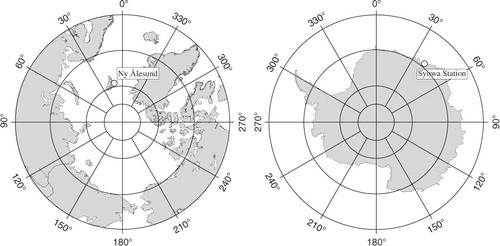
Air samples for the O₂/N₂ ratio measurement have been collected once per week at Ny-Ålesund since 2001 and once or twice per month at Syowa since 2000. Locations of the respective observation sites are shown in Fig. 1. Each air sample was taken from an air intake at a flow rate of 1.8 L min⁻¹ by using a diaphragm pump and filled into a Pyrex glass flask with Viton O-ring seal at ambient pressure after removing water vapour using a cold trap maintained at −78.0°C. The air intake was mounted at the top of an 8 m mast at Syowa and on the roof of a 4 m high observatory hut at Ny-Ålesund. To minimise the deterioration risk of air samples during their storage in the flasks, we used 550 mL flasks at Ny-Ålesund and 2700 mL flasks at Syowa, and each flask filled with sample air was stored in the dark inside of a cardboard box after protecting with a shock-absorbing material. After air sampling, the flasks were stored in on-site laboratory rooms until their transport to Japan, and the sample analysis was carried out as soon as the flasks arrived at Tohoku University. The air samples collected at Ny-Ålesund and Syowa were analysed for the O₂/N₂ ratio within 4 months and 1.5 years, respectively, after their sampling. By analysing the O₂/N₂ ratios of a standard air stored in the 550 mL flasks over 185 days, we confirmed that their values were stable within our analytical precision of flask samples to be described below (Ishidoya et al., 2003). We also found that the O₂/N₂ ratios of the air samples collected into the 2700 mL flasks at Syowa agreed well with the values from our in-situ continuous O₂ measurements at corresponding times at the station (our unpublished data), an average difference between both datasets over the period February 2008 to January 2010 being −3.9±7.5 per meg (flask-in situ). These results imply that permeation of O₂ through the O-ring (Sturm et al., 2004) is insignificant for our sample flasks.

Fig. 1.  Locations of Ny-Ålesund Station, Svalbard, Norway, and Syowa Station, Antarctica.

The O₂/N₂ ratio is reported in per meg unit:1

where subscripts ‘sample’ and ‘standard’ indicate the sample air and the standard air, respectively. Because O₂ is only 20.946% of air, 4.8 per meg of δ(O₂/N₂) corresponds to a change of 1 ppm in the O₂ mole fraction. In this study, δ(O₂/N₂) of each air sample was determined against our working standard air with a reproducibility of ±5.4 per meg (1σ) using a mass spectrometer Finnigan MAT-252 (Ishidoya et al., 2003). The CO₂ concentration value was obtained from the flask sample analyses for Ny-Ålesund and in-situ continuous measurements for Syowa. For concentration determination, a non-dispersive infrared analyzer with a reproducibility of ±0.01 ppm and our gravimetrically prepared air-based CO₂ standard gas system with uncertainties of ±0.13 ppm were used (Nakazawa et al., 1991; Morimoto et al., 2003).

To estimate the variations of APO induced by changes in the air–sea O₂ flux, we used a three-dimensional atmospheric transport model developed at the National Institute of Advanced Industrial Sciences and Technology, Japan, based on the NIRE-CTM 96 model (Taguchi et al., 2002, 2011) (hereafter referred to as STAG). The STAG model has a horizontal resolution of 1.125° and 60 vertical levels and is driven by interannually varying wind fields produced by the operational analysis of European Centre for Medium-Range Weather Forecasts (ECMWF). The air–sea O₂ and N₂ fluxes incorporated into this model are described in the following section.

3. Results and discussion

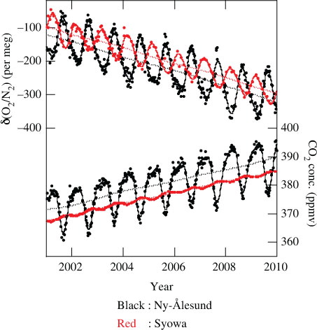
Figure 2 shows the δ(O₂/N₂) and CO₂ concentration values observed at Ny-Ålesund and Syowa for the period January 2001 to December 2009. Best-fit curves to the data and secular trends obtained using a digital filtering technique (Nakazawa et al., 1997) are also shown. In this filtering technique, the average seasonal cycles of δ(O₂/N₂) and CO₂ concentration were approximated by fundamental and its first harmonics, and signals with periods longer than 36 months were regarded as contributing to a secular trend. As can be seen from this figure, δ(O₂/N₂) and the CO₂ concentration show secular decrease and increase, respectively, accompanied by a prominent seasonal cycle at both sites. Such secular changes are mainly attributable to the O₂ utilisation and CO₂ emission during the anthropogenic fossil fuel combustion (Keeling et al., 1996). The average rates of change in δ(O₂/N₂) (CO₂ concentration) at Ny-Ålesund and Syowa over the observation period were −21.2±0.8 (2.00±0.08) and −22.0±0.8 per meg yr⁻¹ (1.99±0.06 ppm yr⁻¹), respectively. The uncertainties of these rates, as well as those of the average seasonal amplitudes of δ(O₂/N₂), CO₂ concentration and APO, were evaluated using a bootstrap method (Press et al., 2007). The measured values of δ(O₂/N₂) (CO₂ concentration) were found to be lower (higher) by about 25 per meg (4 ppm), on average, at Ny-Ålesund than at Syowa, reflecting the fact that the fossil fuel consumption is much larger in the Northern Hemisphere than in the Southern Hemisphere. The respective peak-to-peak amplitudes of the average seasonal δ(O₂/N₂) (CO₂ concentration) cycle at Ny-Ålesund and Syowa were 129±4 (15.2±0.4) and 70±4 per meg (1.10±0.04 ppm). The ratio of the seasonal amplitude of δ(O₂/N₂) at Syowa to that at Ny-Ålesund was 0.54±0.08, which is significantly larger than the corresponding ratio of 0.07±0.01 for the seasonal CO₂ cycle. This difference is ascribed to the fact that the seasonally dependent air–sea O₂ flux and the terrestrial biospheric activity combine to produce the seasonal δ(O₂/N₂) cycle, while the terrestrial biospheric activity is the main contributor to the seasonal CO₂ cycle (Keeling et al., 1993). We also found that the ratio of the seasonal amplitude of δ(O₂/N₂) at Syowa to that at Ny-Ålesund decreased with time at a rate of –0.02±0.01 per meg yr⁻¹. This fact may be attributable to changes in the terrestrial biospheric activity during our observation period, since the seasonal amplitude of CO₂ concentration at Ny-Ålesund gradually increased with time at a rate of 0.24±0.11 ppm yr⁻¹ for this period.

Fig. 2.  Observed values of δ(O₂/N₂) and CO₂ concentration at Ny-Ålesund (black) and Syowa (red). Best-fit curves to the data (solid lines) and secular trends (dotted lines) are also shown.

To extract the oceanic component from the measured values of δ(O₂/N₂), the observed APO was calculated using2

where [CO₂] is the CO₂ mole fraction in ppm, 1.1 is the−O₂:CO₂ molar exchange ratio for the terrestrial biospheric activity (Severinghaus, 1995), 0.20946 is the mole fraction of atmospheric O₂ and 1800 is an arbitrary APO reference point (Stephens et al., 1998). The observed APO values thus calculated for Ny-Ålesund and Syowa are shown in Fig. 3a. Since the average −O₂:CO₂ molar exchange ratio for fossil fuel combustion is 1.4 (Keeling, 1988), which is larger than the ratio of 1.1 for the terrestrial biospheric activity, signals of the fossil fuel combustion still remained in the APO values calculated using eq. (2), showing up as a secular decrease of APO in Fig. 3a. As reported by Van der Laan-Luijkx et al. (2010) and Sirignano et al. (2010), the −O₂:CO₂ molar exchange ratio for fossil fuel combustion is spatially variable in principle. However, it would be plausible for our sites to assume a global mean exchange ratio for fossil fuel combustion because of their remoteness from populated areas. The maximum and minimum of the average seasonal APO cycle at Ny-Ålesund (Syowa) occurred in late August (early March) and in late March (middle September), respectively. The average seasonal peak-to-peak amplitude of APO was found to be 52±3 per meg at Ny-Ålesund and 64±4 per meg at Syowa.

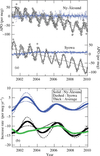
Fig. 3.  (a) Observed values of APO at Ny-Ålesund and Syowa (open circles), and simulated deseasonalised values of APO from the STAG model at these two sites, driven by air–sea O₂ and N₂ fluxes derived from changes in the ocean heat content (blue dots). (b) Increase rates of the observed (black lines) and simulated APO (blue lines). The increase rate of APO corrected for the contribution of interannually varying air–sea O₂ (N₂) flux by subtracting an average of the increase rates simulated for Syowa and Ny-Ålesund from that observed at the two sites is also shown (green line).

To examine the interannual variation of the seasonal APO cycle induced by the atmospheric transport, temporal variations of APO at Ny-Ålesund and Syowa were simulated using the STAG model that incorporated the monthly air–sea O₂ (N₂) flux climatology reported by Garcia and Keeling (2001). The simulated APO values were calculated according to3

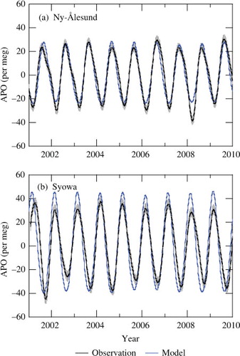
where [O₂] and [N₂] are the simulated concentrations of the respective gases in ppm of dry air, and XO₂ and XN₂ are the respective fractions of O₂ and N₂ in the atmosphere, the corresponding values being 0.20946 and 0.7808. The seasonal cycles of APO derived from the model simulations for both sites are compared in Fig. 4 with the observational results. Although the average seasonal APO cycle was reproduced reasonably well by the model simulations, the simulated year-to-year variation of the seasonal amplitude was significantly underestimated compared to the observation; the simulated amplitudes of the respective years vary in a range of only ±1.4 per meg from their mean at Ny-Ålesund and in a range of only ±1.6 per meg at Syowa, while the observed interannual variability of the amplitude was ±4 per meg at Ny-Ålesund and ±8 per meg at Syowa. This points to the possibility that the air–sea O₂ (N₂) flux is much more important for interannual variations of the seasonal APO cycle than the atmospheric transport. More detailed inspection of the results given in Fig. 4 also reveals that at Syowa, the average simulated seasonal amplitude is slightly larger than the observation. Such a difference in the amplitude could arise from inappropriate seasonality of air–sea O₂ (N₂) flux, especially in the southern hemispheric oceans, and/or atmospheric transport of the model.

Fig. 4.  Comparison of observed and simulated seasonal cycles of APO at Ny-Ålesund and Syowa. The simulated seasonal cycles were obtained using the STAG model that incorporated the monthly air–sea O₂ (N₂) flux climatology. Shades represent uncertainties of the observed seasonal APO cycles.

It has been suggested by previous studies that net oceanic O₂ outgassing is induced by the stratification of the ocean water and the decrease of O₂ solubility in seawater caused by an increase in the upper ocean heat content (e.g. Bopp et al., 2002). Therefore, this effect must be considered when the global CO₂ budget is being estimated from a long-term APO record. For example, Manning and Keeling (2006) and Ishidoya et al. (2012) applied the respective corrections of 0.5 and 0.2 GtC yr⁻¹ to the oceanic CO₂ uptake for the periods 1993–2003 and 2000–2010 by assuming global mean coefficients of 4.9 and 2.2 nmol J⁻¹, respectively, for air–sea fluxes of O₂ and N₂ per heat flux (Keeling and Garcia, 2002).

To examine the effect on the long-term atmospheric APO trend caused by the variation in the air–sea O₂ (N₂) flux (due to changes in the upper ocean heat content), we simulated the APO variations at Ny-Ålesund and Syowa for the period March 1999 to April 2011 using the STAG model forced by temporally varying air–sea O₂ (N₂) fluxes. In this simulation, the contribution from the fossil fuel combustion was not included. The O₂ (N₂) flux at any particular time during the integration was calculated by multiplying 4.9 (2.2) nmol J⁻¹ (Keeling and Garcia, 2002) by the derivative of the upper ocean (0–700 m depth) heat content. The heat content data were taken from the NOAA/NESDIS/NODC Ocean Climate Laboratory database (http://www.nodc.noaa.gov/OC5/3M_HEAT_CONTENT/index.html), which were updated from the results obtained by Levitus et al. (2009). The estimated heat content was based on historical and modern data, correcting for instrumental biases in the bathythermograph records, as well as correcting or excluding some of the Argo float data. It was found from our model simulation that, for both of our sites, the simulated seasonal APO cycle preceded the observed cycle by about 3 months. Therefore, we adjusted the phase of the simulated seasonal APO cycle to agree with the observation. This phase difference could be partly attributable to the fact that an infinite rapid response of the air–sea O₂ (N₂) flux to changes in the ocean heat content was assumed in our model (Keeling et al., 1993). Remaining causes are not well understood yet, but we might be able to note that thermally and marine biologically induced air–sea O₂ exchanges may occur seasonally in different phases and the seasonality of air–sea O₂ (N₂) flux incorporated into our model may not be adequate.

The APO values simulated for Ny-Ålesund and Syowa are shown in Fig. 3a, after subtracting the seasonal cycle derived by applying the digital filtering technique to the simulated results (Nakazawa et al., 1997). As seen from this figure, the simulated APO values show no systematic trend at Ny-Ålesund, while those at Syowa increase by about 8 per meg for the period 2001–2009. This suggests that the oceanic CO₂ uptake estimated using APO observed at Ny-Ålesund and Syowa should be corrected by about 0.0 and 0.4 GtC yr⁻¹, respectively, which is related to the net outgassing of O₂ due to an increase in the upper ocean heat content. These correction values were derived using eqs. (4) and (5) to be described below. The difference between the net O₂ outgassing effects at Ny-Ålesund and Syowa is mainly attributable to the fact that the secular increase rate of the upper ocean heat content is significantly smaller in the Northern Hemisphere (1.4×10²² J yr⁻¹) than in the Southern Hemisphere (4.6×10²² J yr⁻¹) during 2001–2009.

The increase rates of the observed and simulated APO are shown in Fig. 3b. As seen from the figure, their interannual variations are quite similar to each other, both in amplitude and in phase, suggesting that the air–sea O₂ (N₂) fluxes calculated in this study are realistic and are primarily responsible for interannual variability in APO. To correct the observed APO increase rate for the contribution from the interannually varying air–sea O₂ (N₂) flux due to the variation in ocean water properties, we subtracted an average of the simulated increase rates for Syowa and Ny-Ålesund from that observed at the two sites. The result is also shown as a green line in Fig. 3b. Using the resulting ‘corrected’ and observed APO increase rates, we calculated the oceanic and terrestrial biospheric CO₂ uptake in accordance with the equations,4

and5

given by Manning and Keeling (2006). Here, O, F and B are the oceanic CO₂ uptake, anthropogenic CO₂ released from the fossil fuel combustion/cement manufacture, and the terrestrial biospheric CO₂ uptake, respectively (GtC yr⁻¹); and ΔAPO are the observed changes in the atmospheric CO₂ mole fraction in ppm unit and the atmospheric APO in per meg unit, respectively; M_air is the total number of moles of dry air; is the standard mole fraction of O₂ in air (0.20946); α_F and α_B are the global average –O₂:CO₂ molar exchange ratios for fossil fuel combustion (1.39) and the terrestrial biosphere (1.1), respectively. The term Z_eff (GtC yr⁻¹) appeared in the original equation by Manning and Keeling (2006), representing the correction for the contribution of the net oceanic O₂ (N₂) outgassing, is omitted from eq. (5), since such a component has already been included in the corrected increase rate of APO obtained above. In this analysis, the yearly values of CO₂ emitted by the fossil fuel combustion/cement manufacture were taken from the CDIAC database for the period 2001–2008 (Boden et al., 2011), and their preliminary global estimates by CDIAC (http://cdiac.ornl.gov/trends/emis/prelim_2009_2010_estimates.html) were employed for 2009.

Figure 5 shows the oceanic and terrestrial biospheric CO₂ uptake estimated using the above-mentioned method. Also shown are the rates of CO₂ emission from the fossil fuel combustion/cement manufacture (Boden et al., 2011; http://cdiac.ornl.gov/trends/emis/prelim_2009_2010_estimates.html) and of the atmospheric CO₂ increase. The increase rate of atmospheric CO₂ shown in the figure was calculated from the globally averaged marine surface monthly mean data reported by NOAA/ESRL (www.esrl.noaa.gov/gmd/ccgg/trends/). As seen in Fig. 5, the oceanic CO₂ uptake estimated using the APO increase rate corrected for the heat-driven air–sea O₂ (N₂) flux (Fig. 5b) shows significantly smaller interannual variations, compared to that estimated using the observed APO increase rate (Fig. 5a). As a result, the interannual variations of the terrestrial biospheric CO₂ uptake are also reduced. The magnitude of the interannual variations of the oceanic CO₂ uptake is comparable to those derived using an atmospheric inversion (Patra et al., 2005) and an ocean biogeochemical model (McKinley et al., 2004). This implies that a proper correction of the O₂ outgassing effect is crucial for precisely estimating the global CO₂ budget based on APO.

Fig. 5.  (a) Interannual variations of the oceanic and terrestrial biospheric CO₂ uptake estimated using the average increase rate of APO observed at Ny-Ålesund and Syowa, and (b) those using the average increase rate of APO corrected for interannually varying air–sea O₂ (N₂) fluxes induced by changes in the ocean heat content (see text). The rates of CO₂ emission from fossil fuel combustion/cement manufacture and increase of atmospheric CO₂ are also shown. Shades around solid lines with Ocean, Land and Fossil fuel represent uncertainties of their values.

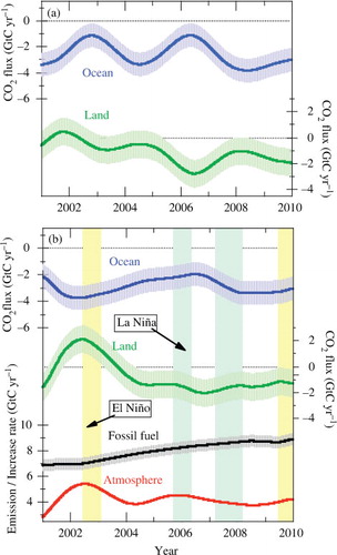
From Fig. 5b, we can also see that the terrestrial biosphere acted as a net source of CO₂ during the 2002–2003 El Niño event when high atmospheric CO₂ increase rates were observed. In this regard, it is noteworthy that Knor et al. (2007) reported, using a terrestrial vegetation model, a global reduction in Net Ecosystem Production (NEP) during 2002–2003 with a large decrease of Net Primary Production (NPP) at northern mid-latitudes. On the other hand, the oceanic CO₂ uptake shows relatively small increase and decrease for the El Niño and La Niña periods, respectively. Nevison et al. (2008b) also reported, using an ocean and terrestrial biogeochemical model combined with a tracer transport model, that the oceanic CO₂ uptake is often increased by about 0.5 GtC yr⁻¹ for the El Niño periods. However, their estimate is slightly smaller than the result of this study.

The average oceanic and terrestrial biospheric uptakes of CO₂ estimated in this study for the period 2001–2009 are 2.9±0.7 and 0.8±0.9 GtC yr⁻¹, respectively. Ishidoya et al. (2012) also showed that APO data taken over Japan yielded an oceanic CO₂ uptake of 2.8±0.7 GtC yr⁻¹ and a terrestrial biospheric CO₂ uptake of 1.0±0.8 GtC yr⁻¹ for the period 2001–2009, by evaluating the net oceanic O₂ (N₂) outgassing using the same method employed in this study. The estimates from the airborne measurements at northern mid-latitude agree well with those from the present boundary-layer measurements at high latitudes. On the other hand, IPCC (2007) reported the average oceanic and terrestrial biospheric CO₂ uptake values for the 1990s to be 2.2±0.4 and 1.0±0.6 GtC yr⁻¹, respectively. By comparing their estimates with ours, it appears that the oceanic CO₂ uptake has recently increased, probably due to a rapid increase in CO₂ emission from the fossil fuel combustion since 2000. If the period of interest is limited to 2004–2009 to exclude the 2002–2003 El Niño effect, the terrestrial biospheric uptake increases to 1.5±0.9 GtC yr⁻¹ and the oceanic uptake decreases slightly to 2.8±0.8 GtC yr⁻¹.

4. Conclusions

We conducted systematic measurements of δ(O₂/N₂) and CO₂ concentration at Ny-Ålesund, Svalbard, and Syowa, Antarctica for the period 2001–2009. APO calculated from measured values of δ(O₂/N₂) and CO₂ concentration showed a prominent seasonal cycle at both sites. By comparing the observed seasonal APO cycles with those simulated using an atmospheric transport model (STAG) with ECMWF wind fields and the TransCom air–sea O₂ (N₂) flux climatology, it was suggested that the main contributor to year-to-year variation of the seasonal amplitude is the interannual variations of the air–sea O₂ (N₂) flux rather than the atmospheric transport. To examine the effect of the air–sea O₂ (N₂) flux on the observed long-term trend of APO, we simulated the APO variations at Ny-Ålesund and Syowa using the STAG model, in which the air–sea O₂ (N₂) flux at any particular time was calculated by multiplying 4.9 (2.2) nmol J⁻¹ by the derivative of the upper ocean heat content taken from the NOAA/NESDIS/NODC Ocean Climate Laboratory database. The observed and simulated interannual variations of the APO increase rate are quite similar to each other, both in amplitude and in phase, suggesting that the air–sea O₂ (N₂) fluxes calculated in this study are primarily responsible for interannual variability in APO.

To correct the observed APO increase rate for the contribution from the interannually varying air–sea O₂ (N₂) flux due to the variation in ocean water properties, we subtracted an average of the simulated increase rates for Syowa and Ny-Ålesund from that observed at the two sites. The oceanic CO₂ uptake estimated using the APO increase rate corrected for the heat-driven air–sea O₂ (N₂) flux showed significantly smaller interannual variations (±0.6 GtC yr⁻¹) compared to that estimated using the observed APO increase rate (±0.9 GtC yr⁻¹). The average oceanic and terrestrial biospheric CO₂ uptake during the period 2001–2009 were estimated to be 2.9±0.7 and 0.8±0.9 GtC yr⁻¹, respectively. From the comparison of the present estimates with those reported by IPCC (2007) for the 1990s, the oceanic CO₂ uptake appears to have increased recently. If the 2002–2003 El Niño period is excluded, the terrestrial biospheric CO₂ uptake for the period 2004–2009 increased to 1.5±0.9 GtC yr⁻¹, while the oceanic uptake decreased slightly to 2.8±0.8 GtC yr⁻¹.

To obtain more reliable estimates of carbon fluxes from the ocean and the terrestrial biosphere, further studies are required for precise estimation of the ocean heat content, as well as for accurate determination of the relationship between the air–sea O₂ (N₂) flux and the heat flux.

Acknowledgments

This study was made as a part of the Science Program of the Japan Antarctic Research Expedition supported by the National Institute of Polar Research (NIPR) under the Ministry of Education, Culture, Sports, Science and Technology (MEXT), Japan, as well as of the NIPR General Collaboration Projects No. 21-17 and Project Research No. KP-10. This study was also partly supported by the Grants-in-Aid for Creative Scientific Research (2005/17GS0203) and the MEXT subsidised project ‘Formation of a virtual laboratory for diagnosing the earth's climate system’. We express our gratitude to the staff of the Norwegian Polar Institute for their cooperation in collecting air samples at Ny-Ålesund, Svalbard.

References

- Bender, M. L, Ho, D. T, Hendricks, M. B, Mika, R, Battle, M. O. and co-authors. 2005. Atmospheric O2/N2 changes, 1993–2002: implications for the partitioning of fossil fuel CO2 sequestration. Global Biogeochem. Cycles. 19: GB4017. DOI: 10.3402/tellusb.v64i0.18924.
- Boden, T. A, Marland, G and Andres, R. J. 2011. Global, Regional, and National Fossil-Fuel CO2 Emissions. US Department of Energy: Oak RidgeTennessee. DOI: 10.3402/tellusb.v64i0.18924.
- Bopp L, Le Quéré C, Heimann M, Manning A. C, Monfray P. Climate-induced oceanic oxygen fluxes: implications for the contemporary carbon budget. Global Biogeochem. Cycles. 2002; 16(2): 1022.10.3402/tellusb.v64i0.18924.
- Garcia H, Keeling R. On the global oxygen anomaly and air-sea flux. J. Geophys. Res. 2001; 106(C12): 31155–31166. 10.3402/tellusb.v64i0.18924.
- IPCC., 2007. Climate Change 2007. “The Physical Science Basis. ” Solomon, S., D.Qin, M.Manning, Z.Chen, M.Marquis, and co-editors. Intergovernmental Panel on Climate Change. Cambridge University Press. 516.
- Ishidoya S, Aoki S, Nakazawa T. High precision measurements of the atmospheric O2/N2 ratio on a mass spectrometer. J. Meteorol. Soc. Japan. 2003; 81: 127–140. 10.3402/tellusb.v64i0.18924.
- Ishidoya, S, Sugawara, S, Hashida, G, Morimoto, S, Aoki, S. and co-authors. 2006. Vertical profiles of the O2/N2 ratio in the stratosphere over Japan and Antarctica. Geophys. Res. Lett. 33: L13701. DOI: 10.3402/tellusb.v64i0.18924.
- Ishidoya, S, Aoki, S, Goto, D, Nakazawa, T, Taguchi, S. and co-authors. 2012. Time and space variations of the O2/N2 ratio in the troposphere over Japan and estimation of global CO2 budget. Tellus. 64B: 18964. DOI: http://dx.doi.org/10.3402/tellusb.v64i0.18964.
- Keeling, R. F. 1988. Development of an Interferometric Oxygen Analyzer for Precise Measurement of the Atmospheric O2 Mole Fraction. Thesis (PhD). Harvard University: Cambridge MA.
- Keeling R. F, Bender M. L, Tans P. P. What atmospheric oxygen measurements can tell us about the global carbon cycle. Global Biogeochem. Cycles. 1993; 7: 37–67. 10.3402/tellusb.v64i0.18924.
- Keeling R. F, Piper S. C, Heimann M. Global and hemispheric CO2 sinks deduced from changes in atmospheric O2 concentration. Nature. 1996; 381(6579): 218–221. 10.3402/tellusb.v64i0.18924.
- Keeling R. F, Garcia H. E. The change in oceanic O2 inventory associated with recent global warming. Proc. Natl. Acad. Sci. USA. 2002; 99: 7848–7853. 10.3402/tellusb.v64i0.18924.
- Knor, W, Gobron, N, Scholze, M, Kaminski, T, Schnur, R. and co-authors. 2007. Impact of terrestrial biosphere carbon exchanges on the anomalous CO2 increase in 2002–2003. Geophys. Res. Lett. 34: L09703. DOI: 10.3402/tellusb.v64i0.18924.
- Levitus, S, Antonov, J. I, Boyer, T. P, Locarnini, R. A, Garcia, H. E. and co-authors. 2009. Global Ocean Heat Content 1955–2008 in light of recently revealed instrumentation problems. Geophys. Res. Lett. 36: L07608. DOI: 10.3402/tellusb.v64i0.18924.
- Manning A. C, Keeling R. F. Global oceanic and land biotic carbon sinks from the Scripps atmospheric oxygen flask sampling network. Tellus. 2006; 58B: 95–116.
- McKinley, G. A, Rödenbeck, C, Gloor, M, Houweling, S and Heimann, M. 2004. Pacific dominance to global air-sea CO2 flux variability: a novel atmospheric inversion agrees with ocean models. Geophys. Res. Lett. 31: L22308. DOI: 10.3402/tellusb.v64i0.18924.
- Morimoto S, Nakazawa T, Aoki S, Hashida G, Yamanouchi T. Concentration variations of atmospheric CO2 observed at Syowa Station, Antarctica from 1984 to 2000. Tellus. 2003; 55B: 170–177.
- Nakazawa, T, Aoki, S, Murayama, S, Fukabori, M, Yamanouchi, T. and co-authors. 1991. The concentration of atmospheric carbon dioxide at Japanese Antarctic station, Syowa. Tellus. 43B: 126–135.
- Nakazawa T, Ishizawa M, Higuchi K, Trivett N. B. A. Two curve fitting methods applied to CO2 flask data. Environmetrics. 1997; 8: 197–218.
- Nevison, C. D, Mahowald, N. M, Doney, S. C, Lima, I. D and Cassar, N. 2008a. Impact of variable air-sea O2 and CO2 fluxes on atmospheric potential oxygen (APO) and land-ocean carbon sink partitioning. Biogeosciences. 5: 875–889. Online at: www.biogeosciences.net/5/875/2008/10.3402/tellusb.v64i0.18924.
- Nevison, C. D, Mahowald, N. M, Doney, S. C, Lima, I. D, van der Werf, G. R. and co-authors. 2008b. Contribution of ocean, fossil fuel, land biosphere, and biomass burning carbon fluxes to seasonal and interannual variability in atmospheric CO2. J. Geophys. Res. 113: G01010. DOI: 10.3402/tellusb.v64i0.18924.
- Patra, P. K, Maksyutov, S, Ishizawa, M, Nakazawa, T, Takahashi, T. and co-authors. 2005. Interannual and decadal changes in the sea-air CO2 flux from atmospheric CO2 inverse modeling. Global Biogeochem. Cycles. 19: GB4013. DOI: 10.3402/tellusb.v64i0.18924.
- Press W. H, Teukolsky S. A, Vetterling W. T, Flannery B. P. Numerical Recipes: The Art of Scientific Computing3rd ed. Cambridge University Press: New York, 2007
- Severinghaus, J. 1995. Studies of the Terrestrial O2 and Carbon Cycles in Sand Dune Gases and in Biosphere 2. Thesis (PhD). Columbia University: New York.
- Sirignano, C, Neubert, R. E. M, Rödenbeck, C and Meijer, H. A. J. 2010. Atmospheric oxygen and carbon dioxide observations from two European coastal stations 2000–2005: continental influence, trend changes and APO climatology. Atmos. Chem. Phys. 10: 1599–1615. DOI: 10.3402/tellusb.v64i0.18924. Online at: www.atmos-chem-phys.net/10/1599/2010/.
- Stephens, B, Keeling, R, Heimann, M, Six, K, Murnane, R. and co-authors. 1998. Testing global ocean carbon cycle models using measurements of atmospheric O2 and CO2 concentration. Global Biogeochem. Cycles. 12(2): 213–230. 10.3402/tellusb.v64i0.18924.
- Sturm, P, Leuenberger, M, Sirignano, C, Neubert, R. E. M, Meijer, H. A. J. and co-authors. 2004. Permeation of atmospheric gases through polymer O-rings used in flasks for air sampling. J. Geophys. Res. 109: D04309. DOI: 10.3402/tellusb.v64i0.18924.
- Taguchi S, Matsueda H, Inoue H. Y, Sawa Y. Long-range transport of CO from tropical ground to upper troposphere: a case study for Southeast Asia in October 1997. Tellus. 2002; 54B: 22–40.
- Taguchi, S, Law, R. M, Rödenbeck, C, Patra, P. K, Maksyutov, S. and co-authors. 2011. TransCom continuous experiment: comparison of 222Rn transport at hourly time scales at three stations in Germany. Atmos. Chem. Phys. 11: 10071–10084. 10.3402/tellusb.v64i0.18924.
- Tohjima, Y, Mukai, H, Machida, T, Nojiri, Y and Gloor, M. 2005. First measurements of the latitudinal atmospheric O2 and CO2 distributions across the western Pacific. Geophys. Res. Lett. 32: L17805. DOI: 10.3402/tellusb.v64i0.18924.
- Van der Laan-Luijkx, I. T, Karstens, U, Steinbach, J, Gerbig, C, Sirignano, C. and co-authors. 2010. CO2, δO2/N2 and APO: observations from the Lutjewad, Mace Head and F3 platform flask sampling network. Atmos. Chem. Phys. 10: 10691–10704. DOI: 10.3402/tellusb.v64i0.18924. Online at: www.atmos-chem-phys.net/10/10691/2010/.