Time and space variations of the O₂/N₂ ratio in the troposphere over Japan and estimation of the global CO₂ budget for the period 2000–2010

ABSTRACT

Systematic measurements of the atmospheric O₂/N₂ ratio have been made using aircraft and ground-based stations in Japan since 1999. The observed seasonal cycles of the O₂/N₂ ratio and atmospheric potential oxygen (APO) vary almost in opposite phase to that of the CO₂ concentration at all altitudes, and their amplitudes and phases are generally reduced and delayed, respectively, with increasing altitude. Simulations of APO using two atmospheric transport models reproduce general features of the observed seasonal cycle, but both models fail to reproduce the phase at an altitude ranging from 8 km to the tropopause. By analysing the observed secular trends of APO and CO₂ concentration, and assuming a global net oceanic O₂ outgassing of 0.2±0.5 GtC yr⁻¹, we estimate global average terrestrial biospheric and oceanic CO₂ uptake for the period 2000–2010 to be 1.0±0.8 and 2.5±0.7 GtC yr⁻¹, respectively.

• O₂/N₂ ratio over Japan
• Atmospheric Potential Oxygen (APO)
• Simulation of APO in the free troposphere
• Terrestrial biospheric CO₂ uptake
• Oceanic CO₂ uptake

1. Introduction

The atmospheric O₂/N₂ ratio has been observed since the early 1990s to estimate terrestrial biospheric and oceanic CO₂ uptake (Keeling et al., 1996). Observations have been carried out at ground-based stations (e.g., Bender et al., 1996; Tohjima et al., 2003; Manning and Keeling, 2006; Stephens et al., 2007), sea-based station (van der Laan-Luijkx et al., 2010), on oceanographic research/commercial vessels (Tohjima et al., 2005; Battle et al., 2006; Thompson et al., 2007), and from aircraft (Langenfelds et al., 1999; Sturm et al., 2005a). Langenfelds et al. (1999), from their measurements over Cape Grim, Australia, reported that the O₂/N₂ ratio between 0 and 1 km altitude decreased secularly, showing a prominent seasonal cycle, in agreement with surface measurements at the same site. Aircraft observations by Sturm et al. (2005a) in the height range of 0.8–3.1 km over Perthshire, United Kingdom, for the period February 2003 to May 2004 also revealed a vertical gradient and seasonal cycle in the O₂/N₂ ratio. More recently, Stephens et al. (2009) and Wofsy et al. (2011) made airborne observations of the O₂/N₂ ratio on a global scale, which covered a height ranging from the surface to 14 km and latitudes between 65°S and 80°N. Their observations contribute to clarifying a global height-latitude O₂ distribution, but the results are limited only during the Airborne Carbon in the Mountains Experiment (ACME-07) campaign in 2007, the Stratosphere-Troposphere Analyses of Regional Transport (START-08) campaign in 2008 and the HIAPER Pole-to-Pole Observations of Atmospheric Tracers (HIPPO) global phase 1 campaign in 2009. In the stratosphere, Ishidoya et al. (2006) have found a long-term decrease of the O₂/N₂ ratio, using a balloon-borne cryogenic air sampler experiment conducted over Japan.

In order to examine temporal and spatial variations of the atmospheric O₂/N₂ ratio in more detail, as well as to estimate the global carbon budget, long-term systematic measurements with aircraft provide crucial information. The O₂/N₂ ratio observed in the free troposphere is largely free from the local influence of O₂ consumption and production at the surface, and its variations reflect O₂ fluxes over a wider geographical area. To that end, we have measured the O₂/N₂ ratio not only at the ground-fixed station in Sendai, Japan, but also in the lower, middle and upper troposphere over Japan for more than a decade, starting in May 1999. In this paper, we present the results of our O₂/N₂ measurements and mainly discuss the seasonal cycle of the O₂/N₂ ratio in the troposphere over Japan, with the aid of 3-D atmospheric chemistry-transport models. We also discuss the terrestrial biosphere and ocean CO₂ uptake estimated using the observed long-term trends of O₂/N₂ ratio and CO₂ concentration.

2. Experimental procedures and model calculations of APO

Air samples were collected once per month (1) in the suburban areas of Sendai, Japan (38°N, 140°E, 150 m.a.s.l.), (2) at altitudes of 2 and 4 km over the Pacific Ocean about 50 km off the coast of Sendai using a chartered light aircraft, Cessna 172, and (3) at an altitude ranging from 8 km to the tropopause (hereafter referred to as ‘8 km-tropopause’) over the main island of Japan between Sendai and Fukuoka (34°N, 130°E) using commercial jet airliners, McDonnell Douglas MD-80 or MD-90 (Nakazawa et al., 1993). The collection of air samples at the surface site was carried out on the roof of a 40-m-high laboratory building on a hill covered mostly with deciduous shrubs. As the urban area of Sendai is located east of our site, the air samples were collected only when winds were westerly. Each air sample was taken from an air intake situated at the western edge of the building by using a diaphragm pump with a flow rate of 1.8 L min⁻¹. The air intake is equipped with an aspirator to prevent fractionation of O₂ and N₂ by thermal diffusion due to radiative heating of the intake (Blaine et al., 2006). Each air sample was filled into a 550-ml Pyrex glass flask with Viton O-ring seal at atmospheric pressure after removing water vapour by a cold trap at −78.0°C.

For the offshore measurements, air samples were taken aboard a Cessna 172 from a specially designed air intake using a diaphragm pump and filled into Pyrex glass flasks with a Viton O-ring seal at ambient pressure. The air samples were not dried, as it is difficult to remove water vapour cryogenically on board the aircraft. We also confirmed that the O₂/N₂ ratio of the air sample was sometimes changed by drying with Mg(ClO₄)₂ by comparing the results from cryogenically dried air samples. Our aircraft is equipped with a tube connected from the front edge of the main wing to the cabin for ventilation, in which fresh air flows by dynamic pressure. Part of the air flowing through the tube was collected so that its principle is the same as the aspirated intake. On the other hand, air sampling on board the MD-80 and MD-90 was conducted using their air conditioning system, and dry air from the so-called ‘fresh air nozzle’ in the cockpit was collected into Pyrex glass flasks with a Viton O-ring seal at cabin pressure. Sturm et al. (2006) reported that the thermal diffusion effect on the O₂/N₂ ratio is negligibly small under air flow velocities of higher than 5 m s⁻¹ at the intake. Because a very large quantity of air is always supplied from the jet engines to the cockpit and the cabin of the MD-80 and MD-90, the thermal diffusion effect would be ignored. The air from the fresh air nozzle is a part of the air from the jet engines so that fractionation of O₂ and N₂ due to the split of air flow line may occur (e.g. Ishidoya et al., 2003). However, as the flow rate of the air from the jet engines is much larger than that from the fresh air nozzle, the fractionation effect would be negligible. The flask samples were brought back to our laboratory and then analysed for the O₂/N₂ ratio and the CO₂ concentration within a few days.

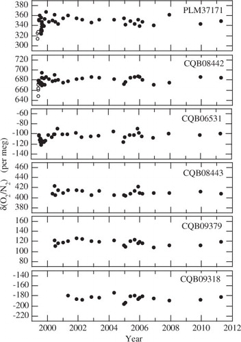
The O₂/N₂ ratio is usually reported in per meg unit:1 where subscripts ‘sample’ and ‘standard’ indicate the sample air and the standard air, respectively. If CO₂ were converted one-for-one into O₂, this would cause an increase of 4.8 per meg of δ(O₂/N₂) for each 1 µmol mol⁻¹ decrease in CO₂. In this study, the δ(O₂/N₂) of each air sample was determined against our working standard air using a mass spectrometer (Finnigan MAT-252). The measurement precision is estimated to be ±5.4 per meg (1 σ). Our air standards, which are classified into primary and working, are dried clean air filled in 48-L high-pressure cylinders. As shown in Fig. 1, our working standards show no systematic trend in the δ(O₂/N₂) with respect to the primary standard (Cylinder No. PLM37172) over the period covered by this study. Details of our δ(O₂/N₂) analysis have been described in Ishidoya et al. (2003). The CO₂ concentration of the air sample was also determined against our air-based CO₂ standard gas system using a non-dispersive infrared analyser (Horiba VIA-500), with a precision of better than ±0.05 ppm (Tanaka et al., 1983). As mentioned above, the air samples collected on board the Cessna 172 were not dried. Therefore, the influence of water vapour on their mass spectrometrically determined δ(O₂/N₂) values was corrected using an experimentally determined relationship between the δ(O₂/N₂) and δ ¹⁵N of N₂ (Ishidoya et al., 2003). Water vapour included in the air sample is decomposed into H⁺ and OH⁻ in the ion source of the mass spectrometer, and the bonding of resultant H⁺ with ¹⁴N¹⁴N (28) produces ¹⁴N¹⁴NH⁺ (29). By this process, the ion beam current of mass 28 decreases and that of mass 29 increases, which leads to higher values of δ ¹⁵N and lower values of δ(O₂/N₂). The amount of the correction varies seasonally, showing the maxima of about 40 per meg at 2 km and 25 per meg at 4 km in July. We also found that the correction is not needed for both heights from winter to spring.

Fig. 1.  δ(O₂/N₂) of 6 standard air samples determined against the primary standard air. Open and closed circles represent the results obtained when the cylinders are standing up and lying down on the floor, respectively.

In order to better understand the variations of δ(O₂/N₂) using atmospheric potential oxygen (APO=O₂+1.1×CO₂), which is conservative for terrestrial biospheric activities (Stephens et al., 1998), we used two 3-D atmospheric transport models: (1) a model developed at the National Institute of Advanced Industrial Sciences and Technology, Japan, based on the NIRE-CTM 96 model (Taguchi, 1996; Taguchi et al., 2002) (hereafter referred to as STAG) and (2) an atmospheric general circulation model (AGCM)-based chemistry-transport model (Patra et al., 2009; hereafter referred to as ACTM). The STAG model has a horizontal resolution of 2.8° and 28° vertical levels. Advection is calculated using a semi-Lagrangian scheme. The STAG model participated in the ‘TransCom’ model intercomparison study (Taguchi et al., 2011). In this study, model simulations were performed using National Center for Environmental Prediction (NCEP) reanalysed meteorological data (NCEP/NCAR for STAG and NCEP/DOE AMIP-II for ACTM). The air–sea O₂ and N₂ fluxes have been taken from the TransCom experimental protocol (Garcia and Keeling 2001; Blaine, 2005). Air–sea CO₂ fluxes from Takahashi et al. (2009) have also been incorporated into the model. To estimate the influence of fossil fuel combustion on the model calculated APO, we also generated variations of the atmospheric CO₂ concentration using only fossil fuel fluxes. The STAG model used emissions from Carbon Tracker (http://www.esrl.noaa.gov/gmd/ccgg/carbontracker; Peters et al., 2007), while the ACTM used those from the Emission Database for Global Atmospheric Research, version 4.0 (EDGAR4, 2009).

APO was calculated using the below equation (Naegler et al., 2007; Nevison et al., 2008):2 where O₂, N₂ and CO₂ are the concentrations in ppm of dry air, APO is expressed in per meg unit, superscripts OC and FF denote ocean and fossil fuel origins, respectively, XO₂ and XN₂ are the fractions of O₂ and N₂ in air, which correspond to 0.2095 and 0.7808, respectively, and 1.4 and 1.1 are the respective molar exchange ratios of O₂ and CO₂ for average fossil fuel combustion (Keeling, 1988) and terrestrial biosphere activities (Severinghaus, 1995). The calculation of APO using the observed parameters is described in Section 3.1.

3. Results and discussion

3.1. Seasonal cycle

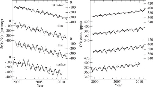
Figure 2 shows our measured δ(O₂/N₂) and CO₂ concentration values. Best-fit curves to the data and long-term trends obtained using a digital filtering technique (Nakazawa et al., 1997a) are also shown. Using this filtering technique, the average seasonal cycle of δ(O₂/N₂) (CO₂ concentration) was approximated by the sum of the fundamental and its first harmonic with the respective periods of 12 and 6 months. The residuals obtained by subtracting the approximated average seasonal cycle from the data were interpolated linearly to calculate daily values of δ(O₂/N₂) (CO₂ concentration). The daily δ(O₂/N₂) (CO₂ concentration) values were smoothed by the 26th-order Butterworth filter with a cutoff period of 36 months to derive the long-term trend. The long-term trend thus obtained was subtracted from the data, and the average seasonal cycle was determined again from the residuals. These steps were repeated until an unchangeable long-term trend obtained.

As evident from Fig. 2, δ(O₂/N₂) decreases gradually with time, in contrast to gradually increasing CO₂ concentration. Both variables vary seasonally at all heights. The average seasonal cycles of δ(O₂/N₂) and CO₂ concentration are shown in Fig. 3. As shown in Fig. 3, the average seasonal cycles of δ(O₂/N₂) and CO₂ concentration at the respective altitudes are shifted by adding their average values over the observation period, to discuss seasonally varying absolute height differences. The average values added were calculated from the best-fit curves to the measured data. The seasonal cycles of δ(O₂/N₂) and CO₂ concentration vary almost in opposite phase at all altitudes, and their amplitudes and phases are generally reduced and delayed, respectively, with increasing altitude. The seasonal maximum of δ(O₂/N₂) appears in early August at the surface, late August at an altitude of 2 km, early September at 4 km and at the beginning of October at 8 km-tropopause. The seasonal minima at those altitudes occur in early March, late March, at the beginning of April and at the beginning of May. On the other hand, the seasonal CO₂ cycle reaches a maximum in late February (surface), middle March (2 km), late March (4 km) and late April (8 km-tropopause), and a minimum in early August, middle August, late August and late September. The respective peak-to-peak amplitudes of δ(O₂/N₂) at the surface, 2, 4 km and 8 km-tropopause are 128±22, 100±23, 83±19 and 43±10 per meg, while the corresponding values for the CO₂ concentration are 13.9±2.5, 11.1±2.3, 9.1±2.3 and 6.4±1.2 ppm. The seasonal cycles of δ(O₂/N₂) and CO₂ concentration observed at the surface are similar to those observed at Cape Ochi-ishi (43°N, 146°E), Japan (Tohjima et al., 2003). However, compared with the results at Heteruma Island (24°N, 124°E) in the southernmost part of Japan (Tohjima et al., 2003), the seasonal amplitudes of δ(O₂/N₂) and CO₂ concentration are almost twice as large, and the seasonal δ(O₂/N₂) maximum and CO₂ minimum occur 1 month earlier. These differences could be attributable to larger seasonal terrestrial biospheric O₂ and CO₂ fluxes at northern middle latitudes than at low latitudes (Nakazawa et al., 1997b). The larger seasonal air–sea O₂ flux at northern middle latitudes than at low latitudes (Garcia and Keeling, 2001) could also contribute to the difference in the seasonal amplitude of δ(O₂/N₂). Sturm et al. (2005b) observed δ(O₂/N₂) and CO₂ concentration at Puy de Dôme (46°N, 3°E, 1480 m.a.s.l.), France, and Jungfraujoch (47°N, 8°E, 3580 m.a.s.l.), Switzerland, and reported peak-to-peak amplitudes of δ(O₂/N₂) and CO₂ concentration to be 190 per meg and 18.2 ppm, respectively, at Puy de Dôme and 79 per meg and 11.0 ppm, respectively, at Jungfraujoch. The seasonal amplitudes of δ(O₂/N₂) and CO₂ concentration at Jungfraujoch are similar to those at 4 km over Japan. However, the amplitudes at Puy de Dôme are significantly larger than our values at 2 km and at the surface. Considering that Puy de Dôme is located in central France, this discrepancy would be ascribed to O₂ and CO₂ fluxes from its surrounding terrestrial biosphere.

Fig. 2.  δ(O₂/N₂) and CO₂ concentration observed in the troposphere over Japan and at the ground surface in the suburbs of Sendai, Japan.

The seasonal CO₂ cycle observed in the Northern Hemisphere is produced mainly by CO₂ exchange between the atmosphere and the terrestrial biosphere through photosynthesis and respiration (Keeling et al., 1989; Nakazawa et al., 1993). The ratio of the change in δ(O₂/N₂) to the change in CO₂ concentration for the average seasonal cycles is calculated to be −7.9, −7.2, −7.9 and −6.0 per meg ppm⁻¹ at the surface, 2, 4 km and 8 km-tropopause, respectively, with the correlation coefficients of 0.91, 0.85, 0.83 and 0.81 in order. These ratios are larger than the −5.3 per meg ppm⁻¹ expected from terrestrial biosphere activities (Severinghaus, 1995). This implies that the oceans contribute to atmospheric O₂ and CO₂ variations in different ways. As mentioned in Keeling et al. (1993), the exchange of CO₂ between the atmosphere and the ocean is highly suppressed due to the carbonate dissociation effect in the ocean, as well as to the counteraction of thermal and biological CO₂ fluxes, while the time scale for equilibration of O₂ between the atmosphere and surface ocean is a few weeks. Thus, thermal and biological O₂ fluxes vary temporally in the same phase. Taking this into account, the observed seasonal cycles of δ(O₂/N₂) are also affected by the air–sea O₂ exchange, in addition to terrestrial biosphere activities.

To examine the oceanic component of δ(O₂/N₂), Stephens et al. (1998) defined APO as,3 where [CO₂] is the CO₂ mole fraction in ppm, 1.1 is the −O₂:CO₂ molar exchange ratio for terrestrial biosphere activities (Severinghaus, 1995), 0.2095 is the atmospheric O₂ mole fraction (Machta and Hughes, 1970) required to convert ppm into per meg and 1800 is an arbitrary APO reference point. We calculated APO by using Eq. (3) to our observational data, and then derived the average seasonal cycle using the same digital filtering technique as above. The average seasonal cycles of APO at the respective altitudes are shown in Fig. 3. It should be noted that the average seasonal cycles at the respective altitudes are shifted again by adding the average values at the corresponding altitudes over the observation period. The seasonal cycle reaches a maximum in early August, early September, late September and late October, and a minimum in early March, late March, early April and early June at the surface, 2, 4 km and 8 km-tropopause, respectively. The seasonal peak-to-peak amplitudes are 52±10, 37±15, 35±13 and 12±7 per meg at the surface, 2, 4 km and 8 km-tropopause, respectively. The seasonal APO cycle observed at the surface is close to those at Cape Ochi-ishi (Tohjima et al., 2003) and La Jolla, USA (33°N, 117°W) (Keeling et al., 1998), which are coastal sites situated at similar latitudes. On the other hand, APO observed at Niwot Ridge, USA (40°N, 106°W, 3397 m.a.s.l.), shows a different seasonal cycle, with a maximum in late September or early October and a peak-to-peak amplitude of about 25 per meg (Keeling et al., 1998), although its latitude is similar to our surface site. The cause is probably attributable to less influence of oceanic O₂ fluxes at Niwot Ridge, as the site is located in a high mountainous area remote from the oceans.

Fig. 3.  Average seasonal cycles of δ(O₂/N₂), CO₂ concentration and APO observed in the troposphere over Japan and at the surface in Sendai (a–c), and average seasonal APO cycles calculated using STAG (solid lines) and ACTM (dashed lines) for the corresponding altitudes (d).

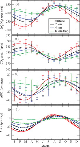
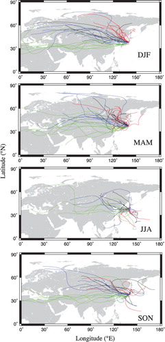
We found APO to be higher in summer and lower in winter at the surface than in the free troposphere. This behaviour is different from that for the CO₂ concentration. In the case of the CO₂ concentration, the surface value is higher than those at 2 and 4 km height throughout the year. To investigate the cause of such high summertime APO values, we calculated 5-d three-D backward trajectories of air parcels released from 0.2, 2 and 4 km over Sendai and 9 km over the midpoint of Sendai and Fukuoka for our observation dates in 2005, 2006 and 2007, using the HYSPLIT model (Draxler and Rolph, 2003; Rolph, 2003; available from NOAA Air Resources Laboratory at http://ready.arl.noaa.gov/HYSPLIT_traj.php). The trajectories obtained are shown in Fig. 4 for four seasons. As seen from the figure, air masses arriving at 2, 4 km and 8 km-tropopause over Japan come mostly from the Eurasian Continent throughout the year. In contrast, many of the air parcels arriving at the surface level in summer originate in the Pacific Ocean. We also confirmed that air parcels arrived at our surface site after travelling at lower altitudes in summer than in the other seasons. This suggests that the high APO values observed at the surface in summer are related to O₂ emitted by enhanced marine biological activity.

Figure 3 also shows the average seasonal cycles of APO calculated using our 3-D atmospheric transport models. In this figure, the average values of APO over the observation period are taken into account to represent the seasonal cycles at the respective altitudes, and the calculated and observed average values of APO at the surface are adjusted to be equal. The models simulate the observed seasonal cycles at the surface, 2 and 4 km fairly well. However, the observed APO for the June–August period is higher at the surface than in the free troposphere, which is not simulated well by the models. This implies that the sea-to-air O₂ fluxes due to marine biological activity around Japan from spring to summer are weak in the models. It should be noted that the air–sea O₂ exchange is produced not only by marine biological activity but also by thermally driven changes in the solubility of O₂ and N₂. However, the effect of the latter on the seasonal APO cycles observed in this study is small. The peak-to-peak amplitudes of the seasonal APO cycles produced by the thermal effect were estimated by STAG (ACTM) to be 9 (6), 5 (5), 3 (4) and 1 (2) per meg for the surface, 2, 4 km and 8 km-tropopause, respectively. These values were obtained based on the seasonal cycles of model-calculated thermally driven atmospheric O₂ and N₂ concentrations; the N₂ concentration was directly calculated from N₂ fluxes taken from the TransCom experimental protocol (Garcia and Keeling, 2001; Blaine, 2005), while the O₂ concentration was deduced by multiplying the calculated N₂ concentration by the ratio of the amplitudes of integrated O₂ and N₂ air–sea fluxes due to temperature changes in the ocean mixed layer (Table 1 in Keeling et al., 1993).

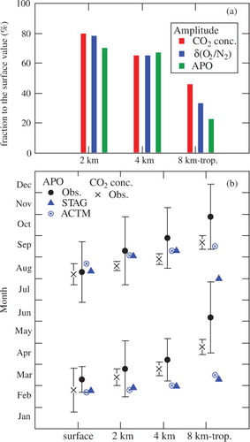
In order to examine the height-dependent seasonal behaviour of δ(O₂/N₂), CO₂ concentration and APO in more detail, their peak-to-peak amplitudes, as well as the appearance times of their seasonal maxima and minima, are summarised as shown in Fig. 5. Observed results show that the amplitudes of all variables decrease with increasing altitude. The decrease relative to the surface value is roughly similar for all variables up to 4 km, but then significantly diverges. Specifically, at 8 km-tropopause, APO and CO₂ concentrations are 22% and 46% of their surface value. The amplitudes of the seasonal APO cycles simulated by both models also decrease with altitude. The calculated amplitudes are generally close to the observed values, but the models show slightly smaller amplitudes than the observational result at the surface. Such an underestimation of the seasonal APO amplitude is also found for La Jolla (Garcia and Keeling, 2001; Battle et al., 2006) using the same air–sea O₂ and N₂ fluxes as used in this study. The decrease of APO seasonal amplitude with height is also reproduced by the models. The data indicate that the seasonal maximum (minimum) of δ(O₂/N₂) and the seasonal minimum (maximum) of the CO₂ concentration at each altitude appear almost simultaneously. The phase delay between the seasonal cycles of δ(O₂/N₂) and CO₂ concentration at the surface and 8 km-tropopause is 1.5–2.0 months. On the other hand, the seasonal APO cycle has a larger phase lag than that for δ(O₂/N₂) and CO₂ concentration in the free troposphere, especially at 8 km-tropopause. The models reproduce the phase of the seasonal APO cycle at the surface and the appearance time of the seasonal maximum at 2 and 4 km fairly well, but fail to simulate the seasonal APO cycle at 8 km-tropopause. The seasonal minima of the simulated APO cycles at 2 and 4 km also appear earlier than the observed timing.

To inspect the seasonality of APO in the Northern Hemisphere, the average seasonal cycle was derived from the data at several coastal surface and high altitude or inland sites. The following coastal sites were considered: Alert (ALT; 82°N, 63°W, 210 m.a.s.l.), Canada (Keeling et al., 1998; Battle et al., 2006); Shetland Island (SIS; 60°N, 1°W), Scotland (Kozlova et al., 2008); Cold bay (CBA; 55°N, 163°W, 25 m.a.s.l.), Alaska, USA (Keeling et al., 1998; Battle et al., 2006); Sendai (this study); and La Jolla (LJO; 33°N, 117°W; Keeling et al., 1998; Battle et al., 2006). For the high altitude/inland sites, we considered: Zotino (ZOTTO; 61°N, 89°E, 114 m.a.s.l.), central Siberia, Russia (Kozlova et al., 2008); Jungfraujoch (JFJ; 47°N, 8°E, 3580 m.a.s.l.; Uglietti et al., 2011); Niwot Ridge (NWR; 40°N, 106°W, 3749 m.a.s.l.; Keeling et al., 1998; Battle et al., 2006); and 4 km and 8 km-tropopause over Japan (this study). The results are plotted as shown in Fig. 6, together with the corresponding model simulations. Evidently, there is good agreement between the observed and STAG-calculated amplitudes at ALT, CBA, ZOTTO, JFJ and NWR, but the model underestimates the amplitude for SIS, Sendai, LJO, and 4 km and 8 km-tropopause over Japan. Similar underestimates are found for SIS (Kozlova et al., 2008) and LJO (Battle et al., 2006). The studies by Kozlova et al. and Battle et al. used the same dataset of air–sea O₂ flux as in this study, but a different atmospheric transport model (TM3). On the other hand, ACTM reproduces the amplitudes at ALT, ZOTTO, NWR, and 4 km and 8 km-tropopause over Japan well, but overestimates that at CBA, as also found by Battle et al. (2006). The agreement between the observed and ACTM-simulated amplitudes at SIS and LJO is reasonably good.

The appearance times of the seasonal APO maxima simulated for the coastal sites are largely consistent with data, but those for the high altitude or inland sites are significantly earlier. Kozlova et al. (2008) also reported that the simulated seasonal APO maximum appears earlier than the observed maximum at ZOTTO. The seasonal APO minima simulated for the coastal sites are found to appear earlier by about one month than in the observations. On the other hand, it is difficult to discuss the phase difference between the observed and simulated APO minima at the high-altitude or inland sites, since the observed seasonal APO cycles at ZOTTO (Fig. 1 in Kozlova et al. 2008), JFJ (Fig. 4 in Uglietti et al. 2011) and NWR (Fig. 2 in Keeling et al. 1998) do not show any clear seasonal minimum. Fig. 6 also shows that the differences in the appearance time between the seasonal APO maxima observed at the high altitude or inland sites and their nearby coastal surface sites are very large, i.e. about 3.5, 2.5, 2.0, 1.5 and 2.5 months for ZOTTO-SIS, JFJ-SIS, NWR-LJO, 4 km over Japan-Sendai and 8 km-tropopause over Sendai, Japan, respectively. Such large time differences for the seasonal APO maximum are, however, not observed in northern low latitudes, specifically, Mauna Loa (20°N, 156°W, 3397 m.a.s.l.) and Kumukai (20°N, 155°W, 40 m.a.s.l.), Hawaii, USA (Keeling et al., 1998), and in the Southern Hemisphere, specifically, the South Pole (90°S, 25°W, 2810 m.a.s.l.) and Syowa Station, Antarctica (69°S, 40°E, 29 m.a.s.l.) (Battle et al., 2006). Our models also reproduced the appearance time of the seasonal APO maximum at Kumukai, Mauna Loa, Syowa and the South Pole fairly well. Therefore, the large delay of the seasonal APO maximum at the high-altitude and inland sites relative to the coastal sites, as well as the significant difference in the appearance time between the observed and simulated seasonal APO maxima, may be a characteristic feature of the northern middle and high latitudes.

Fig. 6.  Peak-to-peak amplitudes and appearance times of the maxima and minima of the average seasonal APO cycles observed at (a) Northern Hemispheric coastal sites and (b) high-altitude and inland sites. The results obtained using STAG and ACTM are also shown.

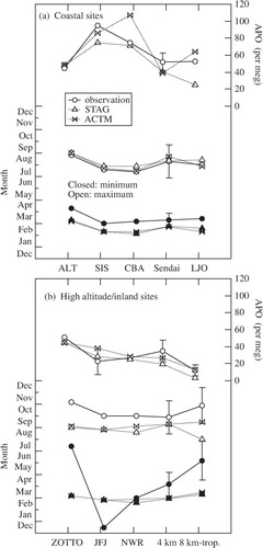
Fig. 4.  Five-d backward trajectories calculated using HYSPLIT for our observation dates in 2005, 2006 and 2007. Red, black, blue and green lines indicate trajectories from the surface in Sendai, 2, 4 km and 8 km-tropopause over Japan, respectively.

Regarding the discrepancy between the observed and model simulated seasonal cycles of APO especially at 8 km-tropopause, it may be noted that Kozlova et al. (2008) examined the seasonal APO cycle at ZOTTO by changing the O₂:CO₂ exchange ratio from 0.9 to 1.2 for terrestrial biospheric activities and found the seasonal maximum to appear earlier by employing the exchange ratios of smaller than 1.1, which leads to a better agreement between the observed and model results. If we tentatively adopt 0.9 for the exchange ratio to derive APO from our observed data of δ(O₂/N₂) and CO₂ concentration at 8 km-tropopause, then the appearance time of the seasonal APO maximum (minimum) occurs earlier by about 2 weeks and the seasonal peak-to-peak amplitude of APO is increased by about 40%, compared to the results for 1.1. The reduction of the O₂:CO₂ exchange ratio improves not only the difference in the phase between the observed and model-simulated seasonal cycles of APO, but also the difference between the fractions of the seasonal amplitude to the surface value for APO and the CO₂ concentration (see Fig. 5a). We also confirmed that the O₂:CO₂ exchange ratio of 1.2 yields a smaller seasonal peak-to-peak amplitude of APO at 8 km-tropopause, compared to that for 1.1. However, by employing smaller O₂:CO₂ exchange ratios for terrestrial biospheric activities, an agreement between the observed and model-simulated seasonal cycles of APO at 2 and 4 km becomes worse. The change of the O₂:CO₂ exchange ratio also affects the long-term trend of APO. Further studies are still needed on the O₂:CO₂ exchange ratio for terrestrial biospheric activities.

Fig. 5.  (a) Fractions of the seasonal CO₂ concentration, δ(O₂/N₂) and APO amplitudes at the respective altitudes to the surface, and (b) appearance times of the maxima and minima of the average seasonal cycles of CO₂ concentration and APO observed in the troposphere over Japan and at the surface in the suburbs of Sendai. Also shown in (b) are the results obtained using STAG and ACTM for APO.

3.2. Estimation of the recent global carbon budget

It is seen from Fig. 2 that δ(O₂/N₂) decreases secularly, in contrast to the CO₂ concentration. Average rates of change of δ(O₂/N₂) and CO₂ concentration over Japan for the period 2000–2010 are estimated to be −22.0±0.5 per meg yr⁻¹ and 2.09±0.03 ppm yr⁻¹, respectively, from the differences between yearly means of the respective variables for 2000 and 2010. An average rate of increase of CO₂ concentration for the 2000–2008 period is calculated to be 1.94±0.04 ppm yr⁻¹, which is very close to the value of 1.95 ppm yr⁻¹ at Mauna Loa for the same period (Keeling et al., 2009). By assuming that our measurements of δ(O₂/N₂) and CO₂ concentration are representative of their globally averaged secular trends, we can estimate the terrestrial biospheric and oceanic CO₂ fluxes from our APO and CO₂ concentration measurements, based on the same analytical method as used by Bender et al. (2005), Manning and Keeling (2006) and Tohjima et al. (2008). This method is basically similar to that proposed by Keeling and Shertz (1992), which solves mass balances for O₂ and CO₂ in the atmosphere using the observed secular trends of δ(O₂/N₂) and CO₂ concentration, but APO is used instead of δ(O₂/N₂). The use of APO has several advantages. For instance, uncertainties in estimated CO₂ fluxes are reduced since short-term (daily to seasonal) variability in APO is smaller than that in δ(O₂/N₂) (Manning and Keeling, 2006). Details of this method are described in the study of Manning and Keeling (2006). The equations derived by them to estimate the net terrestrial biospheric and oceanic CO₂ uptake are given by4 5 where B, F and O are the terrestrial biospheric CO₂ uptake, the anthropogenic CO₂ emitted from fossil fuel combustion and cement manufacture and the oceanic CO₂ uptake, respectively (GtC yr⁻¹); δXco₂ and δAPO are the observed changes in atmospheric CO₂ mole fraction in ppm unit and in atmospheric APO in per meg unit, respectively; M _air and M _c are the total number of moles of dry air (2.12 GtC ppm⁻¹) and the molar mass of carbon (12.01 g mol⁻¹), respectively; Xo₂ is the standard mole fraction of O₂ in air (0.20946), α _F and α _B are the global average O₂:CO₂ molar exchange ratios for fossil fuel combustion (1.38) and the terrestrial biosphere (1.1), respectively; and Z _eff (GtC yr⁻¹) represents the net effect of oceanic O₂ outgassing on the ocean and terrestrial biosphere CO₂ uptake, in which the offset caused by concurrent N₂ outgassing is taken into account. α _F was calculated using CDIAC fossil fuel database for the period 2000–2008 (Boden et al., 2011) and the oxidative ratios for different types of fossil fuel (Steinbach et al., 2011). The net ocean O₂ outgassing is caused mainly by stratification of the ocean and decrease of O₂ solubility in seawater due to an increase in upper ocean heat content (e.g., Bopp et al., 2002), and Manning and Keeling (2006) estimated Z _eff to be 0.5±0.5 GtC yr⁻¹ for the period 1993–2003, which corresponds to an increase of upper ocean heat content of 0.92×10²² J yr⁻¹. We also calculated an average rate of increase of upper ocean heat content for the period 2000–2010 to be 0.42×10²² J yr⁻¹, using the NOAA/NESDIS/NODC Ocean Climate Laboratory data updated by Levitus et al. (2009). On the basis of this calculated increase rate of the upper ocean heat content and the same ratio of air–sea O₂ (N₂) flux to air–sea heat flux as used in Manning and Keeling (2006), we adopted 0.2±0.5 GtC yr⁻¹ for Z _eff in our analysis. Its uncertainties were assumed to be the same as those by Manning and Keeling (2006).

The average rate of change of APO is observed to be −10.9±0.6 per meg for the period 2000–2010. Using this observed rate of APO, together with that of the CO₂ concentration (2.09±0.03 ppm yr⁻¹), we estimated the average terrestrial biospheric and oceanic CO₂ uptake to be 1.0±0.8 and 2.5±0.7 GtC yr⁻¹, respectively. In this analysis, yearly values of CO₂ emitted by fossil fuel combustion and cement manufacture were taken from the CDIAC database for the 2000–2008 period (Boden et al., 2011) and linearly extrapolated to the 2009–2010 period. Errors in the terrestrial biospheric and oceanic CO₂ uptake due to an assumed uncertainty of 6% in the estimates of CO₂ emissions from fossil fuel combustion and cement manufacture (Marland and Rotty, 1984) are estimated to be ±0.48 GtC yr⁻¹. If a value of 0.5±0.5 GtC yr⁻¹ estimated by Manning and Keeling (2006) is adopted for Z _eff, our observational data yield 0.7±0.8 and 2.8±0.7 GtC yr⁻¹ for the average terrestrial biosphere and ocean CO₂ uptake, respectively.

The oceanic and terrestrial biospheric CO₂ uptake estimated from the present and other recent studies based on atmospheric O₂ and CO₂ measurements is summarised in Table 1. Tohjima et al. (2008) reported, from their measurements at Hateruma and Cape Ochi-ishi for the period July 1999–July 2005, that the terrestrial biospheric and oceanic CO₂ uptake was 1.0±0.9 and 2.1±0.7 GtC yr⁻¹, respectively. Our APO and CO₂ concentration data for the 2000–2005 period also yield 1.0±0.9 and 2.5±0.8 GtC yr⁻¹ for the terrestrial biospheric and oceanic CO₂ uptake, respectively, if the same value (0.48±0.48 GtC yr⁻¹) as by Tohjima et al. (2008) is employed for Z _eff. Our terrestrial biospheric CO₂ uptake is very close to that estimated by Tohjima et al. (2008), but our oceanic CO₂ uptake is slightly higher than theirs. The respective terrestrial biospheric and oceanic CO₂ uptake was also estimated to be 1.1±0.6 and 1.8±0.5 GtC yr⁻¹ by Bender et al. (2005) from their O₂ measurements at Cape Grim (41°S, 145°E) for the period June 1993–June 2002, and to be 0.5±0.7 and 2.2±0.6 GtC yr⁻¹ by Manning and Keeling (2006) from their O₂ measurements at La Jolla, Alert and Cape Grim for the period January 1993–January 2003. Tohjima et al. (2008) recalculated the respective values of the terrestrial biospheric and oceanic CO₂ uptake to be 0.6±0.6 and 2.3±0.5 GtC yr⁻¹ for the Bender et al. data and 0.6±0.7 and 2.2±0.6 GtC yr⁻¹ for the Manning and Keeling data, using updated data for global CO₂ changes from the NOAA/ESRL/GMD and fossil fuel CO₂ emissions, and a net ocean O₂ outgassing of 0.48±0.48 GtC yr⁻¹. When compared to our estimates with Z _eff of 0.2 GtC yr⁻¹ for the period 2000–2010, their recalculated terrestrial biospheric and oceanic CO₂ uptake is slightly smaller. The oceanic CO₂ uptake of 1.8 GtC yr⁻¹, estimated by Van der Laan-Luikx et al. (2010) from their measurements at Mace Head, Ireland, for the 1998–2009 period, is much smaller than ours.

Table 1. Oceanic and terrestrial biosphere CO₂ uptake estimated from the present and other recent studies based on atmospheric O₂ and CO₂ measurements

Time period	Data	Ocean sink (GtC yr^−1)	Land sink (GtC yr^−1)
This study 2000–2010	Sendai and over Japan	2.5±0.7	1.1±0.8
Tohjima et al. (2008)	Hateruma, Cape Ochi-ishi	2.1±0.7	1.0±0.9
July 1999–July 2005
Bender et al. (2005)	Cape Grim	1.8±0.5	1.1±0.6
June 1993–June 2002		(2.3±0.5)^a	(0.6±0.6)
Manning and Keeling (2006)	Alert, La Jolla, Cape Grim	2.2±0.6	0.5±0.7
January 1993–January 2003		(2.2±0.6)	(0.6±0.7)
Van der Laan-Luikx et al. (2010) 1998–2009	Mace Head	1.8±0.8

^aThe values in brackets are recalculated values by Tohjima et al. (2008) using the updated data of global CO₂ changes from the NOAA/ESRL/GMD and fossil fuel CO₂ emissions, and the net oceanic O₂ outgassing of 0.48±0.48 GtC yr⁻¹.

As discussed above, there is good agreement between the various estimates of terrestrial biospheric CO₂ uptake based on analysing atmospheric O₂ and CO₂ concentrations (0.6–1.0 GtC yr⁻¹) despite the different measurement periods. On the other hand, the oceanic CO₂ uptake of 2.5±0.7 GtC yr⁻¹ obtained from this study seems to be slightly larger than the values from other studies (1.8–2.3 GtC yr⁻¹). This suggests that oceanic CO₂ uptake has recently increased with time in response to enhanced emissions of fossil fuel CO₂ especially since 2000, although several ocean model simulations indicate a levelling off of the increase in oceanic CO₂ uptake since the mid- to late 1980s (Sarmiento et al., 2010).

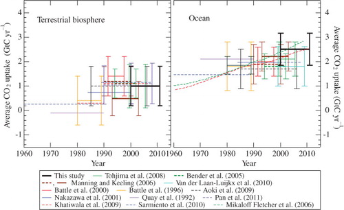
The average terrestrial biospheric and oceanic CO₂ uptake obtained in this study is compared as shown in Fig. 7 with the results estimated using various methods for the period after 1960. This figure indicates that the terrestrial biosphere is not a significant CO₂ source or sink before 1990 and then acts as a CO₂ sink of magnitude 0.5–1.2 GtC yr⁻¹. A rapid increase of terrestrial biospheric CO₂ uptake in the 1990s could be partly related to the Pinatubo eruption in 1991, due to which terrestrial biospheric CO₂ uptake was temporarily enhanced (Jones and Cox, 2001). Our terrestrial biospheric CO₂ uptake agrees well with 1.1±0.8 GtC yr⁻¹ estimated by Pan et al. (2011) for the period 1990–2007 using forest inventory data. The oceanic CO₂ uptake estimated on the basis of the observations indicate an approximate value of 2 (1.7–2.2) GtC yr⁻¹ after 1970, except for this study. On the other hand, the model-based estimates suggest a time-dependent increase of the oceanic CO₂ uptake since the 1960s (Sarmiento et al., 2010), but its value is different between models with time-varying (Sarmiento et al., 2010) and constant ocean circulation (Mikaloff Fletcher et al., 2006). As seen from Fig. 7, the observation-based oceanic CO₂ uptake after 1980 clusters around an average value simulated in the models with time-varying ocean circulation for almost the same period, but our oceanic CO₂ uptake is closer to the result using the model with constant ocean circulation. Our oceanic CO₂ uptake also agrees well with 2.4 GtC yr⁻¹ reported by Khatiwala et al. (2009) for the period 2000–2010, in which a new inverse method was used under an assumption that the tracer transport in the ocean can be described by a Green's function (Note that their oceanic CO₂ uptake after 2009 was obtained personally from S. Khatiwala).

Fig. 7.  Terrestrial biospheric and oceanic CO₂ uptake estimated by the present and other studies for the period after 1960.

4. Conclusions

We have conducted systematic measurements of tropospheric δ(O₂/N₂) in Japan since 1999 using mass spectrometry. δ(O₂/N₂) and APO show a prominent seasonal cycle at the surface, 2, 4 km and 8 km-tropopause, and its amplitude and phase are generally decreased and delayed, respectively, with increasing altitude. APO is higher at the surface than at high altitudes in summer, probably due to the influence of sea-to-air O₂ flux around Japan. Simulations of the seasonal APO cycle using our atmospheric transport models (STAG with Carbon Tracker fossil fuel CO₂ fluxes and ACTM with EDGAR fossil fuel CO₂ fluxes) and the TransCom air–sea O₂ (N₂) fluxes generally reproduce the observed amplitude decrease and phase delay with altitude, but both models fail to reproduce the phase at 8 km-tropopause. The seasonal maximum of APO at high-altitude or inland sites appears significantly later compared with that at nearby surface coastal sites. Such a large phase delay is not reproduced by our models, presumably due to insufficient horizontal and vertical atmospheric transport of O₂ emitted from the oceans. It may be also considered that the assumed 1.1 of exchange ratio for terrestrial biosphere activities is not proper for the calculation of APO at the high altitude and inland sites because choosing of the smaller O₂:CO₂ exchange ratio than 1.1 at 8 km-tropopause reduces the phase differences of the seasonal APO cycles between the observation and models.

Using the observed secular trends of APO and CO₂ concentration at all altitudes for the period 2000–2010, the average terrestrial biospheric and oceanic CO₂ uptake is estimated to be 1.0±0.8 and 2.5±0.7 GtC yr⁻¹, respectively. The terrestrial biospheric CO₂ uptake estimated is consistent with the results from the recent studies based on atmospheric O₂ and CO₂ measurements, but our oceanic CO₂ uptake is higher. Because the present measurement covers a more recent time period than that of other studies, our result could imply that the oceanic CO₂ uptake continues to increase in response to the recent enhancement of fossil fuel CO₂ emission.

High precision measurement of the atmospheric O₂/N₂ ratio is one of the most promising methods for estimating the global carbon budget. However, long-term systematic observations are still limited, especially in the upper troposphere where the only measurements are made by us over Japan. Knowledge of the effect of oceanic O₂ outgassing on the estimation of the global carbon budget, as well as modelling of APO variations, is also still insufficient. Further studies are required not only for an elucidation of spatio-temporal variations of atmospheric O₂ but also for its application to a better understanding of the global carbon cycle.

5. Acknowledgments

We express our gratitude to the staff of Japan Airlines and Toho Air Service for their cooperation while collecting air samples. This study was partly supported by the Grants-in-Aid for Creative Scientific Research (2005)/17GS0203), the Grants-in-Aid for Scientific Research (2006)/18710004) and the subsidized project ‘Formation of a virtual laboratory for diagnosing the earth's climate system’ of the Ministry of Education, Science, Sports and Culture, Japan.

References

- Aoki, S, Nakazawa, T, Terunuma, Y and Ishizawa, M. 2009. Temporal and spatial variations of the concentration and carbon isotopic ratio of atmospheric carbon dioxide in the western Pacific region. T1-036, Proceedings (CD) of 8th International Carbon Dioxide Conference. Jena: Germany.
- Battle M, Bender M, Sowers T, Tans P. P, Butler J. H, co-authors. Atmospheric gas concentrations over the past century measured in air from firn at the South Pole. Nature. 1996; 383(6597): 231–235. 10.3402/tellusb.v64i0.18964.
- Battle M, Bender M. L, Tans P. P, White J. W. C, Ellis J. T, co-authors. Global carbon sinks and their variability inferred from atmospheric O2 and δ13C. Science. 2000; 287: 2467–2470. 10.3402/tellusb.v64i0.18964.
- Battle, M, Fletcher, S, Bender, M, Keeling, R, Manning, A. and co-authors. 2006. Atmospheric potential oxygen: new observations and their implications for some atmospheric and oceanic models. Global Biogeochem. Cycles. 20: GB1010. 10.3402/tellusb.v64i0.18964.
- Bender M, Ellis J. T, Tans P, Francey R, Lowe D. C. Variability in the O2/N2 ratio of southern hemisphere air 1991–1994: implication for the carbon cycle. Global Biogeochem. Cycles. 1996; 10: 9–21. 10.3402/tellusb.v64i0.18964.
- Bender, M. L, Ho, D. T, Hendricks, M. B, Mika, R, Battle, M. O. and co-authors. 2005. Atmospheric O2/N2 changes, 1993–2002: implications for the partitioning of fossil fuel CO2 sequestration. Global Biogeochem. Cycles. 19: GB4017. 10.3402/tellusb.v64i0.18964.
- Blaine, T. W. 2005. Continuous measurements of the atmospheric Ar/N2 ratio as a tracer of air-sea heat flux: models, methods, and data. PhD thesis, University of California: San Diego.
- Blaine T. W, Keeling R. F, Paplawsky W. J. An improved inlet for precisely measuring the atmospheric Ar/N2 ratio. 2006; 6: 1181–1184. 10.3402/tellusb.v64i0.18964.
- Boden, T. A, Marland, G and Andres, R. J. 2011. Global, Regional, and National Fossil-Fuel CO2 Emissions. Carbon Dioxide Information Analysis Center: Oak Ridge National LaboratoryU.S. Department of Energy, Oak Ridge, TN. 10.3402/tellusb.v64i0.18964.
- Bopp L, Le Quéré C, Heimann M, Manning A. C, Monfray P. Climate-induced oceanic oxygen fluxes: implications for the contemporary carbon budget. 2002; 16(2): 1–15. 10.3402/tellusb.v64i0.18964.
- Draxler, R. R and Rolph, G. D. 2003. HYSPLIT (HYbrid Single-Particle Lagrangian Integrated Trajectory) Model access via NOAA ARL READY Website. (http://www.arl.noaa.gov/HYSPLIT.php). NOAA Air Resources Laboratory: Silver SpringMD.
- EDGAR4. 2009, European Commission, Joint Research Centre (JRC)/Netherlands Environmental Assessment Agency (PBL), Emission Database for Global Atmospheric Research (EDGAR), release version 4.0. Online at: http://edgar.jrc.ec.europa.eu.
- Garcia H, Keeling R. On the global oxygen anomaly and air-sea flux. J. Meteorol. Soc. Japan. 2001; 106(C12): 31155–31166. 10.3402/tellusb.v64i0.18964.
- Ishidoya S, Aoki S, Nakazawa T. High precision measurements of the atmospheric O2/N2 ratio on a mass spectrometer. Geophys. Res. Lett. 2003; 81: 127–140. 10.3402/tellusb.v64i0.18964.
- Ishidoya, S, Sugawara, S, Hashida, G, Morimoto, S.,Aoki, S. and co-authors. 2006. Vertical profiles of the O2/N2 ratio in the stratosphere over Japan and Antarctica. Global Biogeochem. Cycles. 33: L13701. 10.3402/tellusb.v64i0.18964.
- Jones C. D, Cox P. M. Modeling the volcanic signal in the atmospheric CO2 record. 2001; 15: 453–465. 10.3402/tellusb.v64i0.18964.
- Keeling R. F. Development of an Interferometric Oxygen Analyzer for Precise Measurement of the Atmospheric O2 Mole Fraction. PhD thesis. Harvard University, Cambridge. 1988
- Keeling C. D, Bacastow R. B, Carter A. F, Piper S. C, Whorf T. P, co-authors. A three-dimensional model of atmospheric CO2 transport based on observed winds: 1. Analysis of observational data. Global Biogeochem. Cycles. 1989; 55: 165–236.
- Keeling R. F, Bender M. L, Tans P. P. What atmospheric oxygen measurements can tell us about the global carbon cycle. 1993; 7: 37–67. 10.3402/tellusb.v64i0.18964.
- Keeling, R. F, Piper, S. C, Bollenbacher, A. F and Walker, J. S. 2009. Atmospheric CO2 records from sites in the SIO air sampling network. In Trends: A Compendium of Data on Global Change. Carbon Dioxide Information Analysis Center. Oak Ridge National Laboratory: U.S. Department of EnergyOak Ridge, TN. 10.3402/tellusb.v64i0.18964. Online at: http://cdiac.ornl.gov/trends/co2/sio-mlo.html.
- Keeling R. F, Piper S. C, Heimann M. Global and hemispheric CO2 sinks deduced from changes in atmospheric O2 concentration. 1996; 381(6579): 218–221. 10.3402/tellusb.v64i0.18964.
- Keeling R. F, Shertz S. R. Seasonal and interannual variations in atmospheric oxygen and implications for the global carbon cycle. Nature. 1992; 358(6389): 723–727. 10.3402/tellusb.v64i0.18964.
- Keeling R. F, Stephens B. B, Najjar R. G, Doney S. C, Archer D, co-authors. Seasonal variations in the atmospheric O2/N2 ratio in relation to the kinetics of air-sea gas exchange. Global Biogeochem. Cycles. 1998; 12: 141–163. 10.3402/tellusb.v64i0.18964.
- Khatiwala, S, Primeau, F and Hall, T. 2009. Reconstruction of the history of anthropogenic CO2 concentrations in the ocean. Nature. 462: 346–349. 10.3402/tellusb.v64i0.18964.
- Kozlova, E. A, Manning, A. C, Kisilyakhov, Y, Seifert, T and Heimann, M. 2008. Seasonal, synoptic, and diurnal-scale variability of biogeochemical trace gases and O2 from a 300-m tall tower in central Siberia. Global Biogeochem. Cycles. 22: GB4020. 10.3402/tellusb.v64i0.18964.
- Langenfelds R. L, Francey R, Steele L. P, Keeling R. F, Bender M, co-authors. Measurements of O2/N2 ratio from the Cape Grim air archive and three independent flask sampling program. Baseline atmospheric program (Australia). 1999; 1996: 57–70.
- Levitus, S, Antonov, J. I, Boyer, T. P, Locarnini, R. A, Garcia, H. E. and co-authors. 2009. Global Ocean Heat Content 1955–2008 in light of recently revealed instrumentation problems. Geophys. Res. Lett. 36: L07608. 10.3402/tellusb.v64i0.18964.
- Machta L, Hughes E. Atmospheric oxygen in 1967 to 1970. Science. 1970; 168: 1582–1584. 10.3402/tellusb.v64i0.18964.
- Manning A. C, Keeling R. F. Global oceanic and land biotic carbon sinks from the Scripps atmospheric oxygen flask sampling network. Tellus. 2006; 58B: 95–116.
- Marland G, Rotty R. M. Carbon dioxide emissions from fossil fuels: a procedure for estimation and results for 1950–1982. Tellus. 1984; 36B: 232–261. 10.3402/tellusb.v64i0.18964.
- Mikaloff Fletcher, S. E, Gruber, N, Jacobson, A. R, Doney, S. C, Dutkiewicz, S. and co-authors. 2006. Inverse estimates of anthropogenic CO2 uptake, transport, and storage by the ocean. Global Biogeochem. Cycles. 20: GB2002. 10.3402/tellusb.v64i0.18964.
- Naegler T, Ciais P, Orr J. C, Aumont O, Roedenbeck C. On evaluating ocean models with atmospheric potential oxygen. Tellus. 2007; 59B: 138–156.
- Nakazawa T, Aoki S, Sugawara S, Ishizawa M, Morimoto S, co-authors. Variations in the concentration and carbon isotopic ratio of tropospheric carbon dioxide over Japan and their implication for the global carbon cycle (extended abstract). Sixth International Carbon Dioxide Conference. 2001; 1: 35–38.
- Nakazawa T, Ishizawa M, Higuchi K, Trivett N. B. A. Two curve fitting methods applied to CO2 flask data. Environmetrics. 1997a; 8: 197–218.
- Nakazawa T, Morimoto S, Aoki S, Tanaka M. Time and space variations of the carbon isotopic ratio of tropospheric carbon dioxide over Japan. Tellus. 1993; 45B: 258–274.
- Nakazawa T, Morimoto S, Aoki S, Tanaka M. Temporal and spatial variations of the carbon isotopic ratio of atmospheric carbon dioxide in the western Pacific region. J. Geophys. Res. 1997b; 102: 1271–1285. 10.3402/tellusb.v64i0.18964.
- Nevison, C. D, Mahowald, N. M, Doney, S. C, Lima, I. D and Cassar, N. 2008. Impact of variable air-sea O2 and CO2 fluxes on atmospheric potential oxygen (APO) and land-ocean carbon sink partitioning. Biogeosciences. 5: 875–889. Online at: www.biogeosciences.net/5/875/2008/10.3402/tellusb.v64i0.18964.
- Pan, Y, Birdsey, R. A, Fang, J, Houghton, R, Kauppi, P. E. and co-authors. 2011. A large and persistent carbon sink in the world's forests. Science. 333: 988–993. 10.3402/tellusb.v64i0.18964.
- Patra P. K, Takigawa M, Dutton G. S, Uhse K, Ishijima K, co-authors. Transport mechanisms for synoptic, seasonal and interannual SF6 variations and “age” of air in troposphere. 2009; 9: 1209–1225. 10.3402/tellusb.v64i0.18964.
- Peters W, Jacobson A. R, Sweeney C, Andrews A. E, Conway T. J, co-authors. An atmospheric perspective on North American carbon dioxide exchange: CarbonTracker. Atmos. Chem. Phys. 2007; 104(48): 18925–18930. 10.3402/tellusb.v64i0.18964.
- Quay P. D, Tilbrook B, Wong C. S. Oceanic uptake of fossil fuel CO2: carbon-13 evidence. Proc. Natl. Acad. Sci. 1992; 256(5053): 74–79. 10.3402/tellusb.v64i0.18964.
- Rolph, G. D. 2003. Real-time Environmental Applications and Display sYstem (READY) Website. NOAA Air Resources Laboratory: Silver SpringMD. Online at: http://www.arl.noaa.gov/ready.php.
- Sarmiento, J. L, Gloor, M, Gruber, N, Beaulieu1, C, Jacobson, A. R. and co-authors. 2010. Trends and regional distributions of land and ocean carbon sinks. , . 7: 2351–2367. Online at: www.biogeosciences.net/7/2351/2010/doi:10.5194/bg-7-2351-201010.3402/tellusb.v64i0.18964.
- Severinghaus J. Studies of the Terrestrial O2 and Carbon Cycles in Sand Dune Gases and in Biosphere 2. Ph D thesis. Columbia University, New York. 1995
- Steinbach J, Gerbig C, Rödenbeck C, Karstens U, Minejima C, co-authors. The CO2 release and oxygen uptake from fossil fuel emission estimate (COFFEE) dataset: effects from varying oxidative ratios. 2011; 11: 6855–6870. 10.3402/tellusb.v64i0.18964.
- Stephens B. B, Bakwin P. S, Tans P. P, TecLaw R. M, Baumann D. Application of a differential fuel-cell analyzer for measuring atmospheric oxygen variations. Atmos. Chem. Phys. 2007; 24: 82–94. 10.3402/tellusb.v64i0.18964.
- Stephens B, Keeling R, Heimann M, Six K, Murnane R, co-authors. Testing global ocean carbon cycle models using measurements of atmospheric O2 and CO2 concentration. Journal of Atmos. and Oceanic Thech. 1998; 12(2): 213–230. 10.3402/tellusb.v64i0.18964.
- Stephens B. B, Shertz S. R, Watt A. S, Bent J. D, Keeling R. F, co-authors. Airborne observation pg atmospheric O2 and CO2 on regional to global scales. Proceedings (CD) of 8th International Carbon Dioxide Conference. Jena, Germany. 2009
- Sturm, P, Leuenberger, M, Moncrieff, J and Ramonet, M. 2005a. Atmospheric O2, CO2 and δ13C measurements from aircraft sampling over Griffin Forest, Perthshire, UK. 19: 2399–2406. 10.3402/tellusb.v64i0.18964.
- Sturm, P, Leuenberger, M and Schmidt, M. 2005b. Atmospheric O2, CO2 and d13C observations from the remote sites Jungfraujoch, Switzerland, and Puy de Dôme, France. Rapid Commun. Mass Spectrom. 32: L17811. 10.3402/tellusb.v64i0.18964.
- Sturm P, Leuenberger M, Valentino F. L, Lehmann B, Ihly B. Measurements of CO2, its isotopes, O2/N2, and 222Rn at Bern, Switzerland. Geophys. Res. Lett. 2006; 6: 1991–2004. 10.3402/tellusb.v64i0.18964.
- Taguchi S. A three-dimensional model of atmospheric CO2 trans-port based on analyzed winds: Model description and simulation results for TRANSCOM. Atmos. Chem. Phys. 1996; 101(D10): 15099–15110. 10.3402/tellusb.v64i0.18964.
- Taguchi S, Law R. M, Rödenbeck C, Patra P. K, Maksyutov S, co-authors. TransCom continuous experiment: comparison of 222Rn transport at hourly time scales at three stations in Germany. J. Geophys. Res. 2011; 11: 10071–10084. 10.3402/tellusb.v64i0.18964.
- Taguchi S, Matsueda H, Inoue H. Y, Sawa Y. Long-range transport of CO from tropical ground to upper troposphere: a case study for Southeast Asia in October 1997. Atmos. Chem. Phys. 2002; 54B: 22–40.
- Takahashi, T, Sutherland, S. C, Wanninkhof, R, Sweeney, C, Feely, R. A and co-authors. 2009. Climatological mean and decadal change in surface ocean pCO2, and net sea-air CO2 flux over the global oceans. Tellus. 56(8–10): 554–577. 10.3402/tellusb.v64i0.18964.
- Tanaka M, Nakazawa T, Aoki S. High quality measurements of the concentration of atmospheric carbon dioxide. Deep–Sea Research II. 1983; 61(4): 678–685.
- Tohjima, Y, Mukai, H, Mschida, T and Nojiri, Y. 2003. Gas-chromatographic measurements of the atmospheric oxygen/nitrogen ratio at Hateruma Island and Cape Ochi-Ichi, Japan. J. Meteorol. Soc. Japan. 30(12): 1653. 10.3402/tellusb.v64i0.18964.
- Tohjima, Y, Mukai, H, Machida, T, Nojiri, Y and Gloor, M. 2005. First measurements of the latitudinal atmospheric O2 and CO2 distributions across the western Pacific. Geophys. Res. Lett. 32: L17805. 10.3402/tellusb.v64i0.18964.
- Tohjima Y, Mukai H, Nojiri Y, Yamagishi H, Machida T. Atmospheric O2/N2 measurements at two Japanese sites: estimation of global oceanic and land biotic carbon sinks and analysis of the variations in atmospheric potential oxygen (APO). Geophys. Res. Lett. 2008; 60B: 213–225.
- Thompson R. L, Manning A. C, Lowe D. C, Wetherburn D. C. A ship-based methodology for high precision atmospheric oxygen measurements and its application in the Southern Ocean region. Tellus. 2007; 59B: 643–653.
- Uglietti, C, Leuenberger, M and Brunner, D. 2011. Large-scale European source and flow patterns retrieved from back-trajectory interpretations of CO2 at the high alpine research station Jungfraujoch. Tellus. 11: 813–857. Online at: www.atmos-chem-phys-discuss.net/11/813/2011/, 10.3402/tellusb.v64i0.18964.
- Van der Laan-Luijkx, I. T, Karstens, U, Steinbach, J, Gerbig, C, Sirignano, C. and co-authors. 2010. CO2, δO2/N2 and APO: observations from the Lutjewad, Mace Head and F3 platform flask sampling network, . 10: 10691–10704. Online at: www.atmos-chem-phys.net/10/10691/2010/, 10.3402/tellusb.v64i0.18964.
- Wofsy, S. C.,The HIPPO Science Team and Cooperating Modellers and Satellite Teams. 2011. HIAPER Pole-to-Pole Observations (HIPPO): fine-grained, global-scale measurements of climatically important atmospheric gases and aerosols. Atmos. Chem. Phys. 369: 2073–2086. 10.3402/tellusb.v64i0.18964.