Modelling temperature acclimation effects on the carbon dynamics of forest ecosystems in the conterminous United States

ABSTRACT

The projected rise in temperature in the 21st century will alter forest ecosystem functioning and carbon dynamics. To date, the acclimation of plant photosynthesis to rising temperature has not been adequately considered in earth system models. Here we present a study on regional ecosystem carbon dynamics under future climate scenarios incorporating temperature acclimation effects into a large-scale ecosystem model, the terrestrial ecosystem model (TEM). We first incorporate a general formulation of the temperature acclimation of plant photosynthesis into TEM, and then apply the revised model to the forest ecosystems of the conterminous United States for the 21st century under the future Intergovernmental Panel on Climate Change (IPCC) Special Report on Emissions Scenarios (SRES) climate scenarios A1FI, A2, B1 and B2. We find that there are significant differences between the estimates of carbon dynamics from the previous and the revised models. The largest differences occur under the A1FI scenario, in which the model that considers acclimation effects predicts that the region will act as a carbon sink, and that cumulative carbon in the 21st century will be 35 Pg C higher than the estimates from the model that does not consider acclimation effects. Our results further indicate that in the region there are spatially different responses to temperature acclimation effects. This study suggests that terrestrial ecosystem models should take temperature acclimation effects into account so as to more accurately quantify ecosystem carbon dynamics at regional scales.

• climate change
• temperature acclimation
• forest ecosystem
• photosynthesis
• carbon dynamics
• TEM

1. Introduction

Recent studies of global climate change suggest that there will be more intense, more frequent and longer lasting heat in future climate. For example, coupled models of climate and terrestrial biosphere functions predict a continuous increase in average global temperatures of between 1.5 and 4°C with CO₂ concentrations rising to between 800 and 1000 ppm (Friedlingstein et al., 2006; Gunderson et al., 2010). In the period 2090–2099, increases in mean surface air temperature and the uncertainty associated with these increases, relative to the period 1980–1999, are estimated to be between 1.8 and 4°C in various emission scenarios using multiple climate models (Meehl et al., 2007). In North America, the annual mean temperature is likely to exceed the global mean in most areas, and average annual temperatures are likely to rise by 2 to 3°C along the western, southern and eastern continental edges and up to more than 5°C in the northern region. Overall warming in the United States is projected to exceed 2°C (Christensen et al., 2007).

These projected increasing temperature feed back to the terrestrial ecosystem and influences the CO₂ exchanges between the land and atmosphere significantly. It is known that plant photosynthesis, which removes CO₂ from the atmosphere, normally steadily rises to an optimum rate with increasing temperature, followed by a relatively rapid decline; additionally, ecosystem respiration, the production portion of the CO₂ flux in the terrestrial ecosystem, potentially increases exponentially with rising temperature. These instantaneous temperature effects on ecosystem carbon dynamics have been modelled (Van't Hoff, 1884; Arrhenius, 1889; Johnson et al., 1942; Farquhar et al., 1980; Raich et al., 1991) and adopted in many large-scale ecosystem models (Raich et al., 1991; Melillo et al., 1993; Running and Hunt, 1993; Bonan, 1995; Chen et al., 1999). However, these models as important components of earth system models have not fully considered the temperature acclimation effects, although some recent analyses with fully-coupled climate-carbon models suggest the potential temperature acclimation of plant photosynthesis is the most important uncertainty in future global carbon cycle estimation (Arneth et al., 2012; Booth et al., 2012). Temperature acclimation is defined as the reversible change that enables optimum functioning under changing environmental conditions (Saxe et al., 2001).

There is growing evidence showing that the response of carbon dynamics in terrestrial ecosystems to temperature is acclimating. For example, Mooney et al. (1978) showed that plants grown at different temperatures exhibit similar rates of net photosynthesis when measured at their growth temperatures. Slatyer (1977) found a linear relationship between optimal and growth temperature with a slope of 0.34°C °C⁻¹ in Eucalyptus pauciflora. Similar slopes were observed or reported in Oxyria digyna (Billings et al., 1971), in Ledum groenlandicum (Smith and Hadley, 1974), in Eucalyptus globulus and E. nitens (Battaglia et al., 1996). Berry and Björkman summarised that plants exhibit considerable differences in their photosynthetic response to temperature and reflect an adaptation to the temperature regimes of their native environments (Berry and Bjorkman, 1980). More recently, Gunderson et al. (2000) conducted laboratory and field studies to examine the impacts of temperature acclimation and suggested that there is potential physiological acclimation of photosynthesis and respiration to temperature in sugar maple. Consequently, Medlyn et al. (2002a, b) recommended that the modelling of forest responses to increasing temperatures should take potential acclimation of the photosynthetic temperature response into account in photosynthesis models (Farquhar et al., 1980). Kattge and Knorr (2007) further derived a general formulation for quantifying the temperature acclimation effect in the parameters established by Farquhar photosynthesis models.

Apart from photosynthesis, studies on the response of plant respiration to temperature have shown that increasing temperature may cause a decline of the Q10, the rate of change in respiration due to a 10°C increase in temperature, leading to lower plant respirations (Wager, 1941; Atkin et al., 2000a; Atkin et al., 2000b; Tjoelker et al., 2001; Covey-Crump et al., 2002; Loveys et al., 2003). This refers to Type I acclimation as proposed by Atkin and Tjoelker (2003) and Atkin et al. (2005). Another form of plant respiration acclimation, Type II acclimation, indicates that there are changes in the overall capacity of plants to perform respiration, resulting in a decrease in the elevation of the temperature response curve with warming. These studies therefore highlighted the need for a better process-based understanding of respiration temperature acclimation and emphasised the importance of considering acclimating plant respiration in large-scale ecosystem models for more successful predictions of the effects of climate change. Several plant respiration acclimation algorithms have been developed, which empirically model plant respiration as an updated function of temperature (Tjoelker et al., 2001; Wythers et al., 2005; King et al., 2006). Based on the existing knowledge, Ziehn et al. (2011) incorporated acclimation mechanisms of plant photosynthesis and respiration into the Biosphere Energy Transfer Hydrology (BETHY) scheme and used plant trait data and a Bayesian approach to quantify the uncertainty of the key parameters in BETHY (Ziehn et al., 2011).

However, there are few studies focusing on incorporating the above knowledge of temperature acclimation into large-scale ecosystem models and examining the differences between estimations of CO₂ exchange between land and atmosphere with and without the coupling of temperature acclimation effects (Smith and Dukes, 2012). Here we build upon existing modelling algorithms and the best available knowledge to study temperature acclimation effects with a large-scale biogeochemical model, the terrestrial ecosystem model (TEM; Zhuang et al., 2003). The revised model is applied to examine the responses of forest ecosystem carbon dynamics to future climate change for the conterminous United States during the 21st century.

2. Materials and methods

2.1. The terrestrial ecosystem model

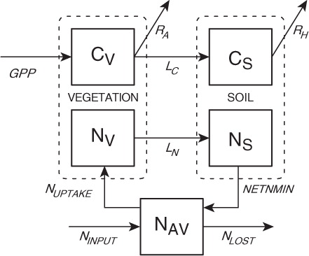
The TEM is a well-documented, process-based ecosystem model that describes the carbon and nitrogen dynamics of plants and soils for terrestrial ecosystems (Raich et al., 1991; McGuire et al., 1992; Melillo et al., 1993; Zhuang et al., 2003; Zhuang et al., 2010). The TEM uses spatially referenced information on climate, elevation, soils, vegetation and water availability as well as soil- and vegetation-specific parameters to make monthly estimates of important carbon and nitrogen fluxes and pool sizes of terrestrial ecosystems. In TEM, carbon fluxes between the biosphere and the atmosphere are modelled as gross primary production (GPP), which represents CO₂ uptake from the atmosphere, and autotrophic respiration (R _A) and heterotrophic respiration (R _H), both of which represent CO₂ emissions from the biosphere (Fig. 1).

Fig. 1.  Schematic diagram of the terrestrial ecosystem model (TEM). Boxes show state variables: vegetation carbon (C_V); vegetation nitrogen (N_V); soil organic carbon (C_S); soil organic nitrogen (N_S); and available soil inorganic nitrogen (N_AV). Arrows show carbon and nitrogen fluxes: gross primary production (GPP); autotrophic respiration (R _A); litterfall carbon (L_C); litterfall nitrogen (L_N); nitrogen uptake by vegetation (N_UPTAKE); net nitrogen mineralization of soil organic nitrogen (NETNMIN); outside nitrogen inputs (NINPUT) and nitrogen loss from the ecosystem (NLOST) (More details, see Raich et al., 1991, McGuire et al., 1992).

GPP (photosynthesis) is modelled as a function of the irradiance of photosynthetically active radiation (PAR), atmospheric CO₂ concentrations, moisture availability, mean air temperature, the relative photosynthetic capacity of the vegetation, and nitrogen availability. The freezing and thawing dynamics have also been considered (Zhuang et al., 2003). The formula for calculating monthly GPP is:1

where C _max is the maximum rate of C assimilation by the entire plant canopy under optimal environmental conditions, and f(PAR), f(P), f(FOLIAGE), f(NA) and f(FT) represent the limits of the photosynthetically active radiation (PAR), the leaf phenology, the influence of relative canopy leaf biomass relative to maximum leaf biomass (Zhuang et al., 2002), the limiting effects of plant nitrogen availability and the effects of freeze-thaw dynamics on GPP (Zhuang et al., 2003), respectively. The term C _A represents the influence of increasing atmospheric CO₂ concentration on GPP, which is modelled by following Michaelis–Menten kinetics (Raich et al., 1991); G _v accounts for changes in leaf conductivity to CO₂ resulting from moisture availability, which is based on the estimates of evapotranspiration (ET). Specifically, f(T) is the temperature scalar with reference to the derivation of optimal temperatures for plant production and T is monthly air temperature, f(T) is modelled as:2

where T _max, T _min, and T _opt are parameters representing maximum, minimum and optimum air temperature for canopy photosynthesis, respectively. Values of f(T) estimated by eq. (2) are limited to a minimum of zero (Raich et al., 1991). Specially, T _opt varies yearly instead of being set as a constant value such as T _max, or T _min. T _opt is set to be the average air temperature of the month in which the f(P) reached its maximum during the previous year, but is limited by two parameters, T _{opt_max} and T _{opt_min} , which provide the upper and lower limits of T _opt, respectively.

R _A is modelled as the sum of maintenance respiration (R _m) and growth respiration (R _g):3

R _m is modelled as a function of vegetation carbon (VEGC) and a scalar indicating the temperature (T) influence:4

where K _r is a parameter representing the respiration rate of the vegetation per unit of biomass carbon at 0°C in grams per gram per month (Raich et al., 1991), which is a function of VEGC. K _rb is a parameter calibrated to fit K _r with VEGC:5

and r _T is the instantaneous rate of change in respiration:6

Instead of using a constant value, Q10, the rate of change in respiration due to a 10°C increase in temperature, has been modelled as a third-order polynomial function to depend on temperature variations:7

The coefficients are determined by fitting the above polynomial to a dataset in which the value of Q10 is about 2 at moderate temperatures between 5 and 20°C, smoothly decreases to 1.5 at high temperatures between 20 and 40°C and increases to 2.5 at low temperatures between 0 and 5°C (McGuire et al., 1992).

R _g is estimated to be 20% of the difference between GPP and R _m. R _H is modelled as a function of soil organic carbon (SOC), soil temperature (T), the influence of soil moisture on decomposition (MOIST), and the gram-specific decomposition constant K _d:8

Net Primary Production (NPP) and Net Ecosystem Production (NEP) in TEM are then defined as:9 10

The version we used in this study is TEM 5.0 (Zhuang et al., 2003), which has coupled a Soil Thermal Model (STM) and a Water Balance Model (WBM), which provide the estimations of thermal and hydrological dynamics to the calculation of carbon cycling processes, but are calculated externally without feedbacks from the carbon cycle.

2.2. Modelling temperature acclimation of photosynthesis

In Farquhar's C3 photosynthesis model (Farquhar et al., 1980), the photosynthesis rate is limited either by RuBP carboxylation or by RuBP regeneration. Two key parameters, V _cmax and J _max, are used as the maximal velocity of RuBP carboxylation and the maximum rate of RuBP regeneration, expressed as the rate of electron transport, which represents plant photosynthetic capacities. An Arrhenius function (Arrhenius, 1889) is normally used to describe the temperature dependence of V _cmax and J _max. Kattge and Knorr (2007) conducted an analysis of data from 36 species to quantify the acclimation to temperature dependence of plant photosynthetic capacities with plant growth temperature, t _growth, which was defined as the average ambient temperature over the canopy during the preceding month. A modified Arrhenius function (Johnson et al., 1942; Medlyn et al., 2002a; Medlyn et al., 2002b) was used to fit observed datasets of V _cmax, J _max and t _growth, and to derive a set of linear relationships between t _growth, key parameters in the modified Arrhenius function (e.g. k ₂₅, the base rate of V _cmax and J _max at the reference temperature of 25°C; H _a, the activation energy, and ΔS, the entropy term in the function), r _J,V (the ratio of the base rates of J _max and V _cmax), and T _opt(V _cmax) and T _opt(J _max) (the optimum temperatures for V _cmax and J _max, respectively):11

where x _i represents key parameters in the modified Arrhenius function and T _opt(V _cmax) and T _opt(J _max), a _i and b _i are acclimation parameters for each x _i . The intercept term a _i indicates the base value of x _i , and the slope b _i represents the temperature acclimation rate. Kattge and Knorr (2007) propose to include the result of regressed temperature acclimation ΔS and r _J,V in eq. (11) to model temperature acclimation effects. Since TEM uses a simpler multiplier [eq. (2)] rather than the Arrhenius function to quantify the temperature dependence of photosynthesis capacity, and the only connection between eq. (11) and TEM's temperature-dependence term is the optimum temperature, we only use the relationships between t _growth and the optimum temperatures when we apply the results provided in eq. (11) to TEM (Table 1).

Table 1. Linear relationship between growth temperature and optimum temperatures [referring to (Kattge and Knorr, 2007) Table 3, used in eq. (12) in this paper]

Parameter	a	SE	b	SE	r ^2
T opt(V cmax)	24.92	1.60	0.44	0.084	0.433
T opt(J max)	26.21	1.17	0.33	0.089	0.385

T _opt(V _cmax) and T _opt(J _max) are the optimum temperature for plant photosynthesis for V _cmax and J _max in Farquhar et al. model.

Although the value of T _opt in TEM is updated yearly as indicated above, it is limited by T _{opt_max} and T _{opt_min} (Table 2), which are estimated based on a compiled dataset (Larcher, 1980; Raich et al., 1991) of current climate (i.e. climate at the end of the 20th century); however, these estimations may not be suitable for the predicted warmer environment in the future. We therefore model the temperature acclimation effect by updating T _{opt_max} and T _{opt_min}. In addition, current values of T _max may also need to be updated with increasing temperature (Kattge and Knorr, 2007). We use the acclimation parameters in eq. (11) for both T _opt (V _cmax) and T _opt (J _max) from Kattge and Knorr (2007) to calculate the temperature-related parameters at each time step in TEM since both of the variables could represent the possible photosynthesis capacity in the model. Therefore, two different sets of parameterisation for acclimation in TEM are conducted based on the rate of acclimation of V _cmax and J _max. Given that the current temperature-related parameters in TEM are T _p,0 and current growth temperature is t _growth,0:12

Table 2. Base temperature-related parameters in TEM for various vegetation types in this study

Vegetation type	T max	T opt_max	T opt_min	T min
Boreal forest	29.0	22.4	14.2	−8.0
Temperate deciduous forest	34.0	30.9	17.0	0.0
Temperate coniferous forest	34.0	30.0	17.0	−1.0

Units are °C.

where the subscript p indicates the temperature-related parameters in TEM including T _{opt_max}, T _{opt_min} and T _max. T _min is assumed to be constant. Also i represents V _cmax or J _max.

At a time step t in the future with growth temperature t _growth,t, we have the acclimated temperature-related parameters:13

Hence the T _p,t(i) is calculated:14

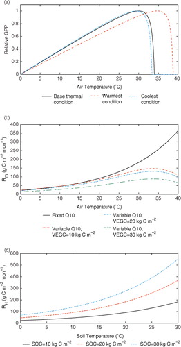
Here we set t _growth,t as the annual average temperature for a given year, which is consistent with the yearly updated T _opt, although the preceding monthly temperature was used for t _growth,t in Kattge and Knorr (2007). Errors induced by this change are evaluated in our study. To examine temperature acclimation effects in the 21st century, we set the base temperature, t _growth,0 as the annual average temperature of the year 2000, the beginning of the 21st century. The parameters in the current version of TEM are used as the base parameters. The modelled effects of air temperature on GPP when t _growth,t increases at different levels, shown in Fig. 2a, demonstrate that the temperature effects on the rates of photosynthesis are low at extreme low and high temperatures and optimum at moderate temperatures, as well as show the shifts of the response relationship under different warming or cooling levels. These effects align with similar trends and patterns as illustrated in Fig. 5 in Kattge and Knorr (2007).

Fig. 2.  Effects of monthly mean temperatures on GPP, R _m and R _H. (a) relative response of GPP to air temperature at different acclimation stages. Base thermal condition: t _growth=21.8°C, T _max=34°C, T _opt=30°C, T _min=0°C; warmest condition: t _growth=34.1°C, T _max=38.7°C, T _opt=34.7°C and T _min=0°C; coolest condition: t _growth=20.2°C, T _max=33.4°C, T _opt=29.4°C and T _min=0°C. b that used for calculating shifts of these parameters is set to be 0.385 as the average of b for T _opt(V _cmax) and T _opt(J _max). Base growth temperatures are extracted as the annual mean air temperature of the grid cell in our regional dataset in 2000; warmest and coolest grow temperatures are determined by the maximum and minimum annual mean air temperature for the same grid. (b) Response of plant maintenance respiration (R _m) to air temperature with fixed Q10=2.0 and variable Q10 that used in TEM with different vegetation carbon pool sizes. Parameter K _rb is set to be a typical value as −5.28. (c) Response of heterotrophic respiration (R _H) to soil temperature at different soil organic carbon pool sizes.

To include the uncertainty of using the linear relationships from the study of Kattge and Knorr (2007), standard errors (SE) of the parameter b _i in eq. (14) are considered in our analysis. Specifically we used b _i ±SE _i to estimate T _p,t(i±SE _i ) in TEM. Therefore six sets of parameters for the acclimation effects are derived including T _p,t(V _cmax), T _p,t(V _cmax+SE_Vcmax), T _p,t(V _cmax−SE_Vcmax), T _p,t(J _max), T _p,t(J _max+SE_Jmax), and T _p,t(J _max−SE_Jmax).

2.3. Temperature acclimation of plant respiration

In TEM, Q10 for plant respiration has been modelled as dynamically dependent on temperature (McGuire et al., 1992) based on a third-order polynomial regression [eq. (7)] which generally follows the Type I acclimation from Atkin and Tjoelker (2003) and Atkin et al. (2005). In this study, we keep the forms of dynamic estimation for Q10 and for the calculations of plant respiration in both the revised and original versions of TEM. Fig. 2b and Fig. 2c show the response of R _m and R _H to temperature with respect to carbon storage with fixed and variable Q10 in our revised TEM.

2.4. Regional simulations

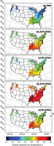
To quantify the effects of temperature acclimation on regional carbon dynamics, we apply the six versions of the revised TEM, as indicated above, to the forest ecosystems of the conterminous United States at a 0.5°×0.5° spatial resolution for the period 1948–2100 with a total of 1370 grid cells (Fig. 3). In order to examine the spatial pattern of the acclimation effect in our study area, we divide the study area into three sub-regions (Southern, Northern and Western) following the Köppen-Geiger climate classification updated map (Kottek et al., 2006). The Southern region represents warm and humid climate, the Northern region represents cold and humid climate, and the Western region represent warm steppe climate. The spatially-explicit soil texture, elevation data and vegetation types are from our previous studies (Melillo et al., 1993; Zhuang et al., 2003). For comparison, the previous version of TEM is also applied for the same region. The climate data from 1948 to 2000 are extracted from NCEP global datasets (Kistler et al., 2001). To examine the carbon response to the most extreme and modest climate scenarios during the 21st century, we use the A1FI, A2, B1 and B2 scenarios from the IPCC SRES (IPCC, 2001). We extract the data from HadCM3 simulated global climate with at a 0.5°×0.5° spatial resolution (Mitchell et al., 2004). The annual atmospheric CO₂ concentration data from 1948 to 2000 are based on data from our previous studies (Melillo et al., 1993). For the period 2001–2100, we retrieve the annual CO₂ concentration data from each of the IPCC SRES scenarios (IPCC, 2001). Temporal variations of annual mean temperatures are shown in Fig. 4. Figure 5 shows the annual maximum temperature in the year 2000, the most extreme scenario A1FI and the modest scenario B1. The temperature generally increases from north to south, and the highest temperature occurs in eastern Texas. In 2000, the highest annual maximum temperature is about 32°C, which rapidly increases to more than 35°C in the 2050s and more than 40°C in the 2090s under the A1FI scenario and increases at a lower rate under the B1 scenario.

Fig. 3.  Potential vegetation coverage of forest region and climatic zones in the conterminous United States at a resolution of 0.5°×0.5° (longitudes×latitudes). The mixed forest is defined in TEM as the combination of 50% deciduous forest and 50% coniferous forest.

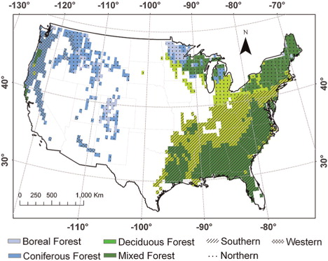
Fig. 4.  Variations of air temperature in the 1990s and the 21st century under the IPCC SRES climate scenarios. ‘max T’, ‘mean T’, ‘min T’ represent the annual maximum, mean and minimum air temperatures, respectively.

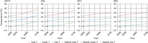
Fig. 5.  Annual maximum air temperature from the monthly dataset of the most extreme and modest climate scenarios (A1FI and B1 respectively) in 2000, and the 2050s as well as 2090s.

For all the simulations, we assume that there is no temperature acclimation before the 21st century. We first run the model to equilibrium and then spin-up the model for 200 yr to account for the influence of climate inter-annual variability on the initial conditions of the ecosystems. During this step, all the simulations are not incorporated with photosynthesis acclimation mechanisms. After that, a group of simulations with and without consideration of acclimation effects are conducted, driven with data of transient climate and annual atmospheric CO₂ concentrations from 1948 to 2100. The results for the whole region and each sub-region from 1990 to 2100 are extracted for further analysis. The emphasis is on examining how acclimation affects the regional estimates of the carbon dynamics of GPP, NPP, NEP, R _A and R _H, as well as vegetation carbon (VEGC) and Soil Organic Carbon (SOC) during the 21st century.

The Euclidean Distance (ED) is used to measure the differences between the simulated time series of carbon dynamics of two models:15

The subscript j indicates the estimated variable (e.g. GPP); V and V′ are the annual values estimated by the previous and revised TEM, respectively. N is 100.

3. Results

3.1. Simulated carbon dynamics with original version of TEM

Both the original and revised TEM estimates for regional forest ecosystems indicated a carbon sink of 0.07±0.1 Pg C yr⁻¹ in the 1990s over the total vegetated area of 3.26 million km². GPP and NPP in the 1990s were 4.7±0.17 and 2.5±0.13 Pg C yr⁻¹, respectively. R _A was estimated to be 2.2±0.06 Pg C yr⁻¹ and R _H was 2.43±0.06 Pg C yr⁻¹. During this period, there was a significant inter-annual variability in carbon fluxes (Figs. 6 and 7).

Fig. 6.  Temporal variations of GPP, NPP and NEP simulated with the previous and the revised versions of TEM from 1990 to 2100 over the study region and each climatic zone. ‘F’ represents GPP, NPP or NEP. The subscript ‘O’ indicates the results estimated by a previous version of TEM and the subscript ‘T’ indicates the results estimated by the revised TEM with incorporation of the temperature acclimation effect. ‘std’ stands for the standard deviation of using T _opt(V _cmax) and T _opt(J _max) and their standard errors in the linear relationship of temperature acclimation.

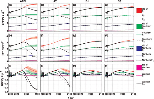
Fig. 7.  Temporal variations of R _A and R _H simulated with the previous and the revised versions of TEM from 1990 to 2100 over the study region and each climatic zone. ‘F’ represents R _A or R _H. The subscripts and ‘std’ have the same meaning in Fig. 6.

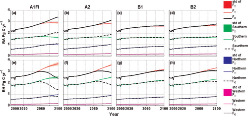
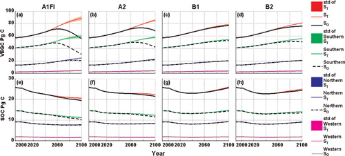
The response of the C dynamics to climate change varied with each of the future climate scenarios (Figs. 6, 7 and 8 6 7 8 ). Under the future climate scenario A1FI, the simulated GPP and NPP increased until the early 2050s but decreased in the remaining years of the 21st century (Fig. 6a,e). Similar trends occurred under the A2 scenario, except that the inflection point occurs 10 yr later (Fig. 6b,f). Instead of inflection, GPP and NPP under the B1 and B2 scenarios show increasing trends (Fig. 6c,d,g,h). NEP had a similar trend (Fig. 6i,j,k,l); however, it slightly decreases after the mid-21st century due to steady increasing R _H under the B1 and B2 scenarios. The respiration trends (R _A and R _H) are highly correlated to the increasing air temperature until the mid-21st century (Fig. 7). Overall, the previous version of TEM estimates higher GPP, NPP and NEP, and R _H, and lower R _A under B1 and B2 than the estimates under the A1FI and A2 scenarios. Variations in carbon pool sizes also occur under the various climate scenarios (Fig. 8). VEGC increases steadily under the B1 and B2 scenarios, but trends decrease after the mid-21st century under the A1FI and A2 scenarios. Conversely, SOC continuously decreasing under the A1FI and A2 scenarios but begins to increase beginning around 2040 under the B1 and B2 scenarios.

Fig. 8.  Temporal variations of VEGC and SOC simulated with the previous and the revised versions of TEM from 1990 to 2100 over the study region and each climatic zone. ‘S’ represents VEGC or SOC. The subscripts and ‘std’ have the same meaning in Fig. 6.

3.2. Simulated carbon dynamics with the revised TEM

The revised TEM simulations are different from the previous version of TEM for the 21st century (Figs. 6, 7 and 8 6 7 8 ). The simulated carbon fluxes continuously increased in the 100-yr period. NEP increases slowly at first but slightly decreases after the mid-21st century. VEGC continues to increase during the study period under all the four climate scenarios. SOC, however, decreases under the A1FI and A2 scenarios, but begins to increase around the mid-21st century under the B1 and B2 scenarios.

The magnitudes of the estimated carbon fluxes and pool sizes are different from the previous results (Table S1). For example, on the annual-average basis, the revised TEM estimates for GPP, NPP and NEP are 0.53, 0.64 and 0.35 Pg C yr⁻¹ higher than those estimated by the previous version under the A1FI scenario, respectively. The revised TEM estimates that R _A is 0.1 Pg C yr⁻¹ lower than the previous results, but that R _H is 0.29 Pg C yr⁻¹ higher. The vegetation carbon and soil organic carbon pool sizes are 7.25 and 0.31 Pg C higher than previous results for the 100-yr period, respectively. Under the A2 scenarios, the differences are similar to A1FI, but the magnitudes are relatively lower. In contrast, the revised and previous versions of TEM estimate similar carbon dynamics under the B1 and B2 scenarios. The revised TEM estimates a little higher GPP, NPP, NEP and R _H but lower R _A than the previous results under these two scenarios; the estimated carbon pool sizes are slightly higher than the previous results.

Table 4. Table S1. Estimated carbon dynamics for the 21st century under the IPCC SRES climate scenarios. The subscript ‘O’ indicates the results estimated by the previous version of TEM and the subscript ‘T’ indicates the results estimated by the revised TEM with incorporating the temperature acclimation effect. ‘Mean’ and ‘std’ stand for the average and the standard deviation of the 100-yr data, respectively.  Supplementary Materials

	A1FI		A2		B1		B2
	Mean	std	Mean	std	Mean	std	Mean	std
Units: Pg C yr^−1
GPPT	5.96	0.66	5.79	0.57	5.57	0.34	5.66	0.40
GPPO	5.43	0.30	5.52	0.32	5.54	0.32	5.57	0.33
NPPT	3.29	0.45	3.19	0.39	3.05	0.25	3.11	0.29
NPPO	2.65	0.41	2.88	0.21	3.01	0.22	3.00	0.20
NEPT	0.26	0.11	0.24	0.09	0.21	0.07	0.23	0.08
NEPO	−0.09	0.33	0.06	0.20	0.19	0.06	0.17	0.07
R AT	2.67	0.21	2.60	0.17	2.52	0.09	2.55	0.11
R AO	2.77	0.34	2.64	0.23	2.53	0.10	2.57	0.13
R HT	3.03	0.38	2.94	0.33	2.84	0.20	2.88	0.24
R HO	2.74	0.18	2.82	0.18	2.82	0.18	2.84	0.19
Units: Pg C
VEGCT	71.99	9.91	70.30	8.44	68.69	6.43	69.51	7.13
VEGCO	64.74	4.60	67.15	5.00	68.12	5.94	68.24	5.85
SOCT	22.20	1.35	23.19	0.68	23.96	0.90	23.66	0.78
SOCO	21.89	1.66	22.95	0.90	23.85	0.81	23.48	0.69

Over the 100-yr period, the revised TEM predicts that the conterminous United States forest ecosystems act as a carbon sink under all four climate scenarios; however, the previous results indicate that the region is a carbon source under the A1FI scenario. The cumulative difference between the 100-yr NEP estimated by the two versions of TEM under the A1FI scenario is as high as 35 Pg C.

4. Discussion

4.1. Temperature effects on carbon fluxes

Extreme temperatures affect carbon dynamics by influencing the biochemical processes of ecosystems. However, plants can offset the negative effects of extreme temperatures through acclimation. For example, a plant acclimated to cold climates can compensate for the low photosynthesis at low temperature conditions by producing leaves with high concentrations of leaf nitrogen and photosynthetic enzymes (Berry and Bjorkman, 1980). Here, the EDs of the two versions indicate there are significant differences in regional carbon dynamics of the conterminous United States forest ecosystems (Table S2).

Table 5. Table S2. Euclidean Distances (ED) between the estimated carbon dynamics by the two versions of TEM under the IPCC SRES climate scenarios in the 21st century. Units are Pg C.

	A1FI	A2	B1	B2
GPP	7.94	4.28	0.36	1.23
NPP	9.72	5.08	0.50	1.56
NEP	4.95	2.87	0.25	0.82
R A	1.87	0.83	0.16	0.35
R H	4.92	2.26	0.28	0.77
VEGC	122.51	56.35	7.77	19.68
SOC	4.74	3.78	1.67	2.75

Air temperature increases rapidly under the A1FI scenario, following with the A2, B2 and B1 scenarios (Fig. 4). The estimation differences between the two versions of the model are on the same order from high to low. As indicated in eq. (2), the rapid increasing air temperature may exceed the optimum and even the maximum temperature for plant photosynthesis at a transition time point and lead to decreasing carbon fixation. The rapidly increasing temperature enhances ecosystem respiration and therefore the net ecosystem production is likely to decrease after the transition time point. The abnormal carbon fluxes lead to the abnormal change in carbon pool sizes (e.g. the temporal trends of the vegetation carbon pool size, VEGC, are positively correlated to NPP, which is the net carbon gain of vegetation). In contrast, with the effect of temperature acclimation, ecosystem carbon fluxes can maintain their trends without a transition time point, and therefore these trends contribute to the significant difference in the results in comparison with the previous version of the model that is not coupled with temperature acclimation effects.

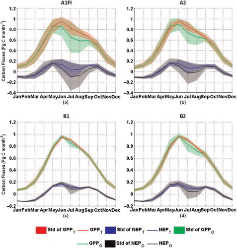
The temperature acclimation effects on carbon fluxes show strong seasonal variations (Fig. 9). Under all climate scenarios, the estimation of GPP and NEP considering the temperature acclimation effect is higher than those estimates obtained without considering the effect during the summer months, but lower during the other months. The annual maximum monthly air temperatures are most likely to occur during the summer months. The largest differences in GPP and NEP estimated by the two versions of the model occur during the summer months, while the differences during the other months are smaller. This suggests that the differences in the estimated annual carbon fluxes mainly occur in summer months and are determined by the maximum air temperature. There are explicit inflections in the trends of GPP, NPP and NEP simulated with the previous TEM under the A1FI and A2 scenarios (Fig. 6). The inflection points are around 2050 and 2060 under the A1FI and A2 scenarios, respectively. For our study region, the maximum monthly air temperature under the A1FI scenario is 29.5°C in 2050, and 29.4°C in 2060 under the A2 scenario. This suggests that, for the forest ecosystems of the conterminous United States, 29.5°C may be the transition point of plant carbon assimilation from an ascending to a descending trend with increasing air temperature.

Fig. 9.  Seasonal variations of estimated GPP and NEP in the 21st century under the IPCC SRES climate scenarios. The plots are the 100-yr average values and the ‘std’ represents the standard deviation of the 100-yr results.

Apart from the temperature acclimation of photosynthesis, possible acclimation effects on plant respiration (Atkin et al., 2005) also have to be taken into account. Since both the revised and original TEM simulations account for the Type I acclimation of plant respiration [eq. (11)], the significantly lower estimates of R _A by the revised versions of TEM are most likely caused by the indirect impacts of incorporating the temperature acclimation of photosynthesis. This might help to partly explain the Type II acclimation of plant respiration proposed in Atkin and Tjoelker (2003) and Atkin et al. (2005). As shown in Figs. 6 and 8, the revised versions of TEM estimate higher GPP and NPP, especially under the A1FI and A2 scenarios, resulting in more carbon accumulation in VEGC. Referring to eq. (3, 4 and 5), both the parameters K _r and VEGC provide the base rate of the maintenance respiration; however, K _r is inversely correlated to VEGC. Figure 2b shows how VEGC can influence the maintenance respiration in TEM; these relationships are similar to the Fig. 4c in Smith and Dukes (2012). The mechanism of Type II acclimation of plant respiration is not fully understood to date, although many studies have presented evidence, such as changes in capacity per mitochondrion (Klikoff, 1966), differences in the number of mitochondria per unit area (Miroslavov and Kravkina, 1991), or changes in plant nitrogen and carbohydrate concentrations (Stockfors and Linder, 1998; Gunderson et al., 2000). These studies suggest that Type II acclimation is largely associated with temperature-mediated changes in respiratory capacity (Atkin and Tjoelker, 2003). Considering these new findings, the parameter K _r might have been too simply modelled in our study, which may lead to the large differences in R _A estimates.

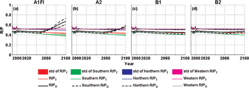
Although the short-term temperature dependences of photosynthesis and plant respiration are different (i.e. respiration is assumed to be more sensitive to temperature than photosynthesis), many lines of evidence suggest that temperature acclimation may be able to create a balance between plant photosynthesis and respiration, leading to an insensitive ratio of plant respiration and photosynthesis (R/P) to temperature (Gifford, 1994; Gifford, 1995; Gifford, 2003). Dewar et al. (1999) suggested that acclimated R/P may depend mainly on the internal allocation of carbohydrates to protein synthesis. Atkin et al. (2005) further indicated that the maintenance R/P probably reflects the fact that photosynthesis and plant respiration are interdependent. As shown in our study, the original TEM, without incorporating photosynthesis acclimation, predicts an increasing R/P in the 21st century, while the revised versions estimate a steadier R/P, suggesting that the revised TEM might have estimated more reasonable regional carbon dynamics (Fig. 10).

Fig. 10.  Variations of estimated ratio of plant respiration and photosynthesis (R/P) by the previous and the revised versions of TEM from 1990 to 2100 over the study region and each climatic zone. The subscripts and ‘std’ have the same meaning in Fig. 6.

Acclimation of soil respirations has also been found (Oechel et al., 2000; Luo et al., 2001; Melillo et al., 2002; Curiel Yuste et al., 2010). Luo et al. (2001) indicated the temperature sensitivity of soil respiration (Q10) decreases under warming, and increases at low temperatures through acclimation. Janssens and Pilegaard (2003) presented similar conclusions, finding large seasonal changes in the Q10 of soil respiration in a beech forest. Giardina and Ryan (2000) provided evidence showing that the decomposition rates of organic carbon in mineral soil do not vary with temperature. However, a number of studies have attributed this apparent acclimation to other factors. For example, Allison et al. (2010) suggested that declines in microbial biomass and degradative enzymes can explain the observed attenuation of soil respiration under warming. Sampson et al. (2007) suggested that variation in photosynthetic signatures induces different seasonal changes in the base rate of soil respiration via differences in the belowground supply of labile carbon. Since the mechanisms of soil respiration acclimation are still not fully elucidated, temperature acclimation of R _H has not been explicitly considered in this study (i.e. dynamic Q10); however, temperature acclimation of R _H has been implicitly accounted for as a result of the interactions among ecosystem processes in TEM. For instance, with the revised version of TEM, while more carbon is fixed by plants, more litterfall carbon is produced, resulting in higher SOC (Figs. 6, 7 and 8 6 7 8 ). Higher SOC results in higher R _H, although this may be partly regulated by the stress of soil moisture availability (Fig. 2c).

4.2. Spatial patterns of carbon dynamics

The conterminous United States spans various climate zones (Peel et al., 2007). The forest ecosystem response to increasing temperature and the temperature acclimation effect may vary spatially in the region. We examine the contributions of the three sub-regions to the temporal variations of the carbon fluxes and pool sizes and temperature acclimation effect (i.e. the differences between model estimations with and without acclimation) over our study region. As shown in Figs. 6, 7, 8, 10 and 6 7 8 ^{Fig. 10.} 12, the Southern region contributes the most to temporal carbon and water dynamics and explains most of the acclimation effect. In contrast, the contribution of the Northern region mostly happens in the late 21st century under the A1FI and A2 scenarios, but the contribution becomes little under the B1 and B2 scenarios. The Western region seems to contribute the least. These spatial patterns are mostly due to the differences in area and climatic environment between these regions.

We examined the spatial pattern of the different responses under the most extreme climate change scenario, A1FI. We find the differences between GPP and NEP estimated by the previous and revised TEM in the 2090s are large in most of the Southern region but low in most of the Northern and Western regions (Fig. 11). The Northern and Western regions are cooler than the tropical and subtropical area in the South, with the annual maximum monthly temperature averaging less than 25°C in 2000 (Fig. 5a). During the 21st century, rising temperatures may lead to increases in T _{opt_max}, T _max and T _opt in the revised model. For the Northern and Western regions in the first half of the 21st century, the acclimated T _opt may still be in the range of the upper and lower limitations in both the previous and the revised versions of TEM; therefore, the acclimation of T _opt may not cause the differences between the estimates of the two versions of the model. However, since T _max is also acclimated in the revised model, according to eq. (2), the revised model may estimate a lower GPP, leading to a lower NEP in the Northern region for that period (Fig. 11). In contrast, the annual maximum monthly temperatures in the Southern region are already close to the initial T _{opt_max} in the year 2000; therefore, the increasing T _opt will have a positive effect on the carbon assimilation in the Southern regions, resulting in a higher GPP and NEP with the revised TEM (Fig. 11). In conclusion, the base growth temperature can be important in determining the direction of the temperature acclimation effect, resulting in a spatial heterogeneity of carbon simulation differences between two versions of the model.

Fig. 11.  Spatial distribution of the differences between GPP and NEP estimated by the two versions of TEM under the A1FI climate scenario. The differences are calculated by the revised TEM GPP and NEP minus the results estimated by the previous version of TEM.

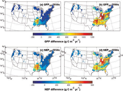
Regions with higher GPP and NEP estimated by the revised TEM seem to be spreading with the rising air temperature. As shown in Fig. 11, during the 2050s, negative GPP and NEP differences occur only in the low-latitude area of the Southern region. However, during the 2090s, only cold regions in the northeast with high latitudes, the Rocky Mountain area and the Pacific Northwest area exhibit negative differences in GPP and NEP. The largest positive differences occur in forest ecosystems in the middle-latitudes, because the annual maximum monthly temperature in that region may be the closest to the acclimated T _opt while the temperatures in the south may have exceeded the optimum value.

4.3. Limitations and uncertainties

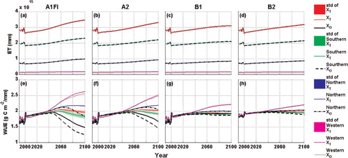
Plant acclimation occurs through a series of biochemical and physiological processes. Plants make physiological adaptations by keeping a physiological process closer to a homeostatic rate than would be expected based on short-term responses. This adjustment may be due to a variety of environmental factors or limitations other than temperature. For example, short-term elevated levels of atmospheric CO₂ often accelerate photosynthesis (Norby et al., 2005), yet plants may down-regulate photosynthetic activity over longer timeframes through physiological and biochemical adjustments (Ainsworth and Long, 2008; Lee et al., 2011). The Michaelis–Menten kinetics incorporated in TEM only account for the fertilisation effect of rising atmospheric CO₂ concentrations, but no acclimation mechanisms are considered. Additionally, more frequent drought may happen, accompanied by global warming in the future (Dai, 2011). While water stress can result in a reduction in plant photosynthesis and respiration rates by reducing leaf stomata openness in the short term, the plants may be able to survive through acclimation (Shinozaki and Yamaguchi-Shinozaki, 2007; Fulda et al., 2011). We calculate the evapotranspiration (ET) and Water Use Efficiency (WUE), which is defined as GPP/ET, to investigate the effects of water stress on photosynthesis. We find that ET is positively correlated to temperature increases under all climate scenarios and WUE is steadier than values from the original TEM estimates (Fig. 12). The more adequate analysis on how water stress affects acclimation shall be conducted with more recent versions of TEM that incorporate the effects of changing plant canopy due to carbon dynamics on hydrological cycling (Felzer et al., 2009). In addition, acclimation of photosynthesis and respirations to other factors such as nutrient availability and irradiance and their interactive effects should also be considered in future analysis (Maxwell et al., 1994; Valladares and Pearcy, 1997; Atkin et al., 2005).

Fig. 12.  Variations of ET and WUE simulated with the previous and the revised versions of TEM from 1990 to 2100 over the study region and each climatic zone. ‘X’ represents either ET or WUE. The subscripts and ‘std’ have the same meaning in Fig. 6.

Four major uncertainty sources should be discussed. First, we adopt a general linear relationship from (Kattge and Knorr, 2007) to estimate the acclimated temperature-related parameters in TEM using a 1-yr time-scale. In contrast, the time-scale was one month in (Kattge and Knorr, 2007). To test the uncertainty of the choice of time-scale for temperature acclimation, we run the model using 1-month and 10-yr time-scales under the A1FI climate scenario. The comparison shows that the differences between these scales are much smaller than the differences due to incorporating the temperature acclimation effect (Table 3). Although the differences are not significant in our study, more attention is necessary for global studies, since more dramatic seasonal and inter-annual temperature variations may occur relative to our regional study. Since the linear relationship is produced based on the Farquhar's photosynthesis model with the reanalysed data of 36 species, the limited data points and the uncertainty of the relationship could bias the temperature-related parameters, and consequently the carbon dynamics. For example, Lin et al. (2012) showed that factors such as photosynthetic biochemistry, respiration and vapour pressure deficit also affect the temperature response of plant photosynthesis. Thus future development of acclimation algorithms should also take these factors into account. In addition, since TEM and Farquhar's approaches are different in modelling the temperature effects on photosynthesis, the choice of T _opt for V _cmax and J _max in TEM may also contribute to the uncertainty. To test these hypotheses, we conduct a set of ensemble simulations using the temperature parameters calculated for V _cmax and J _max with the coefficient b plus-or-minus its standard error (SE). The standard deviation (std) of the ensemble simulations is used to account for this uncertainty (Figs. 6, 7, 8, 6 7 8 10 and 12). Generally the uncertainty of the carbon fluxes or pool sizes is higher under the climate scenarios in which air temperature increases more rapidly (e.g. A1FI and A2), and is larger when temperature increases.

Table 3. Differences of the estimated carbon dynamics in the 21st century between using 1-yr time-scale of temperature acclimation, 1-month, and 10-yr time-scales

Time-scale	GPP	NPP	NEP	RA	RH	VEGC	SOC
1-month	−0.0094	−0.0106	−0.0071	0.0012	−0.0035	−0.1019	−0.0080
10-yr	0.0270	0.0314	0.0184	−0.0044	0.0130	0.3590	0.0423

The numbers are calculated by using 1-yr time-scale results minus the results with other time-scales. Units are Pg C yr⁻¹.

Second, the indirect acclimation of plant respiration and soil respiration was modelled through changing carbon pools affected by photosynthesis acclimation, although the function of direct temperature acclimation has been proposed in (Atkin et al., 2008). However, the acclimation of respirations is still not fully understood and more quantitative evidence is needed before being incorporated into ecosystem models (Atkin et al., 2005).

Third, there is a spatial and inter-species heterogeneity in the temperature acclimation. In our study we incorporate a general linear relationship for temperature acclimation for all the forest types across the conterminous United States. However, many studies have shown that the degree of the acclimation is highly diverse in different species and in different regions (Mooney et al., 1978; Huner et al., 1993; Dewar et al., 1999; Bunce, 2000; Gunderson et al., 2000; Gunderson et al., 2010). Thus, future study should consider the spatial and inter-species heterogeneity of acclimation in response to temperature variations when more data are available. Finally, the acclimation effects on the dynamics of vegetation succession and competition that are important for estimating carbon exchange between the terrestrial biosphere and the atmosphere are not yet in our model (Foley et al., 1996; Sitch et al., 2003). These acclimation effects in dynamic global vegetation models should help quantify carbon dynamics that are regulated by both ecosystem structure and functioning (Bachelet et al., 2001; Lenihan et al., 2003).

5. Summary and conclusions

This study explores the effects of temperature acclimation on the carbon dynamics of forest ecosystems over the conterminous United States during the 21st century. We find that the significance of the temperature acclimation effect on carbon dynamics varies under different climate scenarios. The largest differences occur under the A1FI scenario, with a cumulative carbon sink of 35 Pg C higher than the previous estimates with an earlier version of TEM. The differences are relatively small under the A2, B1 and B2 scenarios because of their lower air temperature increases. In addition, there is a large spatial heterogeneity of carbon assimilations in response to the temperature acclimation effect. This is primarily due to the asynchronous increasing of the optimum temperature for photosynthesis and the air temperature in the region. Our study suggests that quantifying the future net carbon exchange should consider the temperature acclimation effects on both photosynthesis and plant and soil respiration. Developing more observational data on temperature acclimation for various ecosystem types should be a research priority.

Acknowledgments

This study is supported through a project (EAR-0630319) of NSF Carbon and Water in the Earth Program, a CDI-Type II project (IIS-1028291), NASA Land Use and Land Cover Change program with a project (NASA-NNX09AI26G), and a US Department of Energy project (DE-FG02-08ER64599). The computing is supported by Rosen Center of high performance computing at Purdue. We also thank Ms. Jayne Piepenburg for English proofreading.

References

- Ainsworth E. A, Long S. P. What have we learned from 15 years of free-air CO2 enrichment (FACE)? A meta-analytic review of the responses of photosynthesis, canopy properties and plant production to rising CO2. New Phytol. 2008; 165: 351–372. 10.3402/tellusb.v65i0.19156.
- Allison S. D, Wallenstein M. D, Bradford M. A. Soil-carbon response to warming dependent on microbial physiology. Nature Geosci. 2010; 3: 336–340. 10.3402/tellusb.v65i0.19156.
- Arneth A, Mercado L, Kattge J, Booth B. B. B. Future challenges of representing land-processes in studies on land-atmosphere interactions. Biogeosci. 2012; 9: 3587–3599. 10.3402/tellusb.v65i0.19156.
- Arrhenius S. On the reaction velocity of the inversion of cane sugar by acids. Zeitschrift für physikalische Chemie. 1889; 4: 226–248.
- Atkin O. K, Edwards E. J, Loveys B. R. Response of root respiration to changes in temperature and its relevance to global warming. New Phytol. 2000a; 147: 141–154. 10.3402/tellusb.v65i0.19156.
- Atkin O. K, Holly C, Ball M. C. Acclimation of snow gum (Eucalyptus pauciflora) leaf respiration to seasonal and diurnal variations in temperature: the importance of changes in the capacity and temperature sensitivity of respiration. Plant Cell Environ. 2000b; 23: 15–26. 10.3402/tellusb.v65i0.19156.
- Atkin O. K, Tjoelker M. G. Thermal acclimation and the dynamic response of plant respiration to temperature. Trends Plant Sci. 2003; 8: 343–351. 10.3402/tellusb.v65i0.19156.
- Atkin O. K, Bruhn D, Hurry V. M, Tjoelker M. G. The hot and the cold: Unravelling the variable response of plant respiration to temperature. Funct. Plant Biol. 2005; 32: 87–105. 10.3402/tellusb.v65i0.19156.
- Atkin, O. K, Atkinson, L. J, Fisher, R. A, Campbell, C. D, Zaragoza-Castells, J. and co-authors. 2008. Using temperature-dependent changes in leaf scaling relationships to quantitatively account for thermal acclimation of respiration in a coupled global climate–vegetation model. Glob. Change Biol. 14: 2709–2726.
- Bachelet D, Neilson R. P, Lenihan J. M, Drapek R. J. Climate change effects on vegetation distribution and carbon budget in the United States. Ecosystems. 2001; 4: 164–185. 10.3402/tellusb.v65i0.19156.
- Battaglia M, Beadle C, Loughhead S. Photosynthetic temperature responses of eucalyptus globulus and eucalyptus nitens. Tree Physiol. 1996; 16: 81–89. 10.3402/tellusb.v65i0.19156.
- Berry J, Bjorkman O. Photosynthetic response and adaptation to temperature in higher plants. Ann. Rev. Plant Physiol. 1980; 31: 491–543. 10.3402/tellusb.v65i0.19156.
- Billings W. D, Godfrey P. J, Chabot B. F, Bourque D. P. Metabolic acclimation to temperature in Arctic and alpine ecotypes of oxyria digyna. Arctic Alpine Res. 1971; 3: 277–289. 10.3402/tellusb.v65i0.19156.
- Bonan, G. B. 1995. Land-atmosphere CO2 exchange simulated by a land surface process model coupled to an atmospheric general circulation model. J. Geophys. Res. 100: 2817–2831. 10.3402/tellusb.v65i0.19156.
- Booth, B. B, Jones, C. D, Collins, M, Totterdell, I. J, Cox, P. M. and co-authors. 2012. High sensitivity of future global warming to land carbon cycle processes. Environ. Res. Lett. 7: 024002.10.3402/tellusb.v65i0.19156.
- Bunce J. Acclimation of photosynthesis to temperature in eight cool and warm climate herbaceous C3 species: Temperature dependence of parameters of a biochemical photosynthesis model. Photosynth. Res. 2000; 63: 59–67. 10.3402/tellusb.v65i0.19156.
- Chen J. M, Liu J, Cihlar J, Goulden M. L. Daily canopy photosynthesis model through temporal and spatial scaling for remote sensing applications. Ecol. Model. 1999; 124: 99–119. 10.3402/tellusb.v65i0.19156.
- Christensen, J. H, Hewitson, B, Busuioc, A, Chen, A, Gao, X. and co-authors. 2007. Regional Climate Projections. In: Climate Change 2007: The Physical Science Basis. Contribution of Working Group I to the Fourth Assessment Report of the Intergovernmental Panel on Climate Change. Solomon, S., D.Qin, M.Manning, Z.Chen, M.Marquis and co-editors.Cambridge University Press: CambridgeUnited Kingdom and New York, NY, USA. pp. 848–940.
- Covey-Crump E. M, Attwood R. G, Atkin O. K. Regulation of root respiration in two species of Plantago that differ in relative growth rate: the effect of short- and long-term changes in temperature. Plant Cell Environt. 2002; 25: 1501–1513. 10.3402/tellusb.v65i0.19156.
- Curiel Yuste, J, Ma, S and Baldocchi, D. D. 2010. Plant-soil interactions and acclimation to temperature of microbial-mediated soil respiration may affect predictions of soil CO2 efflux. Biogeochemistry: An International Journal. 98: 127–138. 10.3402/tellusb.v65i0.19156.
- Dai A. Drought under global warming: a review. Wiley Interdisciplinary Reviews: Climate Change. 2011; 2: 45–65. 10.3402/tellusb.v65i0.19156.
- Dewar R. C, Medlyn B. E, McMurtrie R. E. Acclimation of the respiration/photosynthesis ratio to temperature: insights from a model. Glob. Change Biol. 1999; 5: 615–622. 10.3402/tellusb.v65i0.19156.
- Farquhar G. D, Caemmerer S, Berry J. A. A biochemical model of photosynthetic CO2 assimilation in leaves of C3 species. Planta. 1980; 149: 78–90. 10.3402/tellusb.v65i0.19156.
- Felzer B. S, Cronin T. W, Melillo J. M, Kicklighter D. W, Schlosser C. A. Importance of carbon-nitrogen interactions and ozone on ecosystem hydrology during the 21st century. J. Geophys. Res. 2009; 114: G01020.10.3402/tellusb.v65i0.19156.
- Foley, J. A, Prentice, I. C, Ramankutty, N, Levis, S, Pollard, D. and co-authors. 1996. An integrated biosphere model of land surface processes, terrestrial carbon balance, and vegetation dynamics. Global Biogeochem. Cycles. 10: 603–628. 10.3402/tellusb.v65i0.19156.
- Friedlingstein, P, Cox, P, Betts, R, Bopp, L, von Bloh, W. and co-authors. 2006. Climate–Carbon Cycle Feedback Analysis: Results from the C4MIP Model Intercomparison. Journal of Clim. 19: 3337–3353. 10.3402/tellusb.v65i0.19156.
- Fulda S, Mikkat S, Stegmann H, Horn R. Physiology and proteomics of drought stress acclimation in sunflower (Helianthus annuus L.). Plant Biol. 2011; 13: 632–642. 10.3402/tellusb.v65i0.19156.
- Giardina C. P, Ryan M. G. Evidence that decomposition rates of organic carbon in mineral soil do not vary with temperature. Nature. 2000; 404: 858–861. 10.3402/tellusb.v65i0.19156.
- Gifford R. The global carbon cycle: A viewpoint on the missing sink. Australian J. Plant Physiol. 1994; 21: 1–15. 10.3402/tellusb.v65i0.19156.
- Gifford R. Whole plant respiration and photosynthesis of wheat under increased CO2 concentration and temperature: long-term vs. short-term distinctions for modelling. Glob. Change Biol. 1995; 1: 385–396. 10.3402/tellusb.v65i0.19156.
- Gifford R. Plant respiration in productivity models: Conceptualisation, representation and issues for global terrestrial carbon-cycle research. Funct. Plant Biol. 2003; 30: 171–186. 10.3402/tellusb.v65i0.19156.
- Gunderson C. A, Norby R. J, Wullschleger S. D. Acclimation of photosynthesis and respiration to simulated climatic warming in northern and southern populations of Acer saccharum: laboratory and field evidence. Tree Physiol. 2000; 20: 87–96. 10.3402/tellusb.v65i0.19156.
- Gunderson C. A, O'Hara K. H, Campion C. M, Walker A. V, Edwards N. T. Thermal plasticity of photosynthesis: the role of acclimation in forest responses to a warming climate. Glob. Change Biol. 2010; 16: 2272–2286. 10.3402/tellusb.v65i0.19156.
- Huner, N, Öquist, G, Hurry, V, Krol, M, Falk, S. and co-authors. 1993. Photosynthesis, photoinhibition and low temperature acclimation in cold tolerant plants. Photosynth. Res. 37: 19–39. 10.3402/tellusb.v65i0.19156.
- IPCC. 2001. Climate Change 2001: Synthesis Report. A Contribution of Working Groups I, II, and III to the Third Assessment Report of the Intergovernmental Panel on Climate Change. Cambridge University Press: Cambridge, United Kingdom and New York NY.
- Janssens I. A, Pilegaard K. Large seasonal changes in Q10 of soil respiration in a beech forest. Glob. Change Biol. 2003; 9: 911–918. 10.3402/tellusb.v65i0.19156.
- Johnson F. H, Eyring H, Williams R. W. The nature of enzyme inhibitions in bacterial luminescence: Sulfanilamide, urethane, temperature and pressure. J. Cell Compar Physl. 1942; 20: 247–268. 10.3402/tellusb.v65i0.19156.
- Kattge J, Knorr W. Temperature acclimation in a biochemical model of photosynthesis: a reanalysis of data from 36 species. Plant Cell Environ. 2007; 30: 1176–1190. 10.3402/tellusb.v65i0.19156.
- King A. W, Gunderson C. A, Post W. M, Weston D. J, Wullschleger S. D. Plant Respiration in a Warmer World. Science. 2006; 312: 536–537. 10.3402/tellusb.v65i0.19156.
- Kistler, R, Collins, W, Saha, S, White, G, Woollen, J. and co-authors. 2001. The NCEP–NCAR 50-year reanalysis: Monthly means CD–ROM and documentation. Bull. Am Meteorol. Soc. 82: 247–267.
- Klikoff L. G. Temperature dependence of the oxidative rates of mitochondria in danthonia intermedia, penstemon davidsonii and sitanion hystrix. Nature. 1966; 212: 529–530. 10.3402/tellusb.v65i0.19156.
- Kottek M, Grieser J, Beck C, Rudolf B, Rubel F. World Map of the Köppen-Geiger climate classification updated. Meteorologische Zeitschrift. 2006; 15: 259–263. 10.3402/tellusb.v65i0.19156.
- Larcher W. Psyiological Plant Ecology. New York, Springer-Verlag. 1980
- Lee T. D, Barrott S. H, Reich P. B. Photosynthetic responses of 13 grassland species across 11 years of free-air CO2 enrichment is modest, consistent and independent of N supply. Glob. Change Biol. 2011; 17: 2893–2904. 10.3402/tellusb.v65i0.19156.
- Lenihan J. M, Drapek R, Bachelet D, Neilson R. P. Climate change effects on vegetation distribution, carbon, and fire in California. Ecol Appl. 2003; 13: 1667–1681. 10.3402/tellusb.v65i0.19156.
- Loveys, B. R, Atkinson, L. J, Sherlock, D. J, Roberts, R. L, Fitter, A. H. and co-authors. 2003. Thermal acclimation of leaf and root respiration: an investigation comparing inherently fast- and slow-growing plant species. Glob. Change Biol. 9: 895–910. 10.3402/tellusb.v65i0.19156.
- Luo Y, Wan S, Hui D, Wallace L. L. Acclimatization of soil respiration to warming in a tall grass prairie. Nature. 2001; 413: 622–625. 10.3402/tellusb.v65i0.19156.
- Maxwell C, Griffiths H, Young A. J. Photosynthetic acclimation to light regime and water stress by the C3-CAM epiphyte guzmania monostachia: Gas-exchange characteristics, photochemical efficiency and the xanthophyll cycle. Funct. Ecol. 1994; 8: 746–754. 10.3402/tellusb.v65i0.19156.
- McGuire, A. D, Melillo, J. M, Joyce, L. A, Kicklighter, D. W, Grace, A. L. and co-authors. 1992. Interactions between carbon and nitrogen dynamics in estimating net primary productivity for potential vegetation in North America. Global. Biogeochem. Cy. 6: 101–124. 10.3402/tellusb.v65i0.19156.
- Medlyn, B. E, Dreyer, E, Ellsworth, D, Forstreuter, M, Harley, P. C. and co-authors. 2002a. Temperature response of parameters of a biochemically based model of photosynthesis. II. A review of experimental data. Plant Cell Environ. 25: 1167–1179. 10.3402/tellusb.v65i0.19156.
- Medlyn B. E, Loustau D, Delzon S. Temperature response of parameters of a biochemically based model of photosynthesis. I. Seasonal changes in mature maritime pine (Pinus pinaster Ait.). Plant Cell Environ. 2002b; 25: 1155–1165. 10.3402/tellusb.v65i0.19156.
- Meehl, G. A, Stocker, T. F, Collins, W. D, Friedlingstein, P, Gaye, A. T. and co-authors. 2007. Global Climate Projections. In: Climate Change 2007: The Physical Science Basis. Contribution of Working Group I to the Fourth Assessment Report of the Intergovernmental Panel on Climate Change. Solomon, S., D.Qin, M.Manning, Z.Chen, M.Marquis and co-editors. Cambridge University Press: CambridgeUnited Kingdom and New York, NY, USA. pp. 749–845.
- Melillo, J. M, McGuire, A. D, Kicklighter, D. W, Moore, B, Vorosmarty, C. J. and co-authors. 1993. Global climate change and terrestrial net primary production. Nature. 363: 234–240. 10.3402/tellusb.v65i0.19156.
- Melillo, J. M, Steudler, P. A, Aber, J. D, Newkirk, K, Lux, H. and co-authors. 2002. Soil warming and carbon-cycle feedbacks to the climate system. Science. 298: 2173–2176. 10.3402/tellusb.v65i0.19156.
- Miroslavov E. A, Kravkina I. M. Comparative analysis of chloroplasts and mitochondria in leaf chlorenchyma from mountain plants grown at different altitudes. Ann. Bot-London. 1991; 68: 195–200.
- Mitchell, T. D, Carter, T. R, Jones, P. D, Hulme, M and New, M. 2004. A comprehensive set of high-resolution grids of monthly climate for Europe and the globe: the observed record (1901–2000) and 16 scenarios (2001–2100). Tyndall Working Paper No. 55, Tyndall Centre, Norwich, UEA.
- Mooney H. A, Bjorkman O, Collatz G. J. Photosynthetic acclimation to temperature in the desert shrub, Larrea divaricata: I. Carbon dioxide exchange characteristics of intact leaves. Plant Physiol. 1978; 61: 406–410. 10.3402/tellusb.v65i0.19156.
- Norby, R. J, DeLucia, E. H, Gielen, B, Calfapietra, C, Giardina, C. P. and co-authors. 2005. Forest response to elevated CO2 is conserved across a broad range of productivity. Proceedings of the National Academy of Sciences of the United States of America. 102: 18052–18056. 10.3402/tellusb.v65i0.19156.
- Oechel, W. C, Vourlitis, G. L, Hastings, S. J, Zulueta, R. C, Hinzman, L. and co-authors. 2000. Acclimation of ecosystem CO2 exchange in the Alaskan Arctic in response to decadal climate warming. Nature. 406: 978–981. 10.3402/tellusb.v65i0.19156.
- Peel M. C, Finlayson B. L, McMahon T. A. Updated world map of the Köppen-Geiger climate classification. Hydrol. Earth Syst. Sci. 2007; 11: 1633–1644. 10.3402/tellusb.v65i0.19156.
- Raich, J. W, Rastetter, E. B, Melillo, J. M, Kicklighter, D. W, Steudler, P. A. and co-authors. 1991. Potential Net Primary Productivity in South America: Application of a Global Model. Ecol Appl. 1: 399–429. 10.3402/tellusb.v65i0.19156.
- Running, S. W and Hunt, E. R.Jr. 1993. Generalization of a forest ecosystem process model for other biomes, BIOME-BGC, and an application for global-scale models. In: Scaling Physiological Processes: Leaf to Globe. Ehleringer, J. R. and C. B Field. Academic Press: San DiegoCA, pp. 141–158.
- Sampson D, Janssens I, Curiel Yuste J, Ceulemans R. Basal rates of soil respiration are correlated with photosynthesis in a mixed temperate forest. Glob. Change Biol. 2007; 13: 2008–2017. 10.3402/tellusb.v65i0.19156.
- Saxe H, Cannell M. G. R, Johnsen Ø, Ryan M. G, Vourlitis G. Tree and forest functioning in response to global warming. New Phytol. 2001; 149: 369–399. 10.3402/tellusb.v65i0.19156.
- Shinozaki K, Yamaguchi-Shinozaki K. Gene networks involved in drought stress response and tolerance. J. Exp. Bot. 2007; 58: 221–227. 10.3402/tellusb.v65i0.19156.
- Sitch, S, Smith, B, Prentice, I, Arneth, A, Bondeau, A. and co-authors. 2003. Evaluation of ecosystem dynamics, plant geography and terrestrial carbon cycling in the LPJ dynamic global vegetation model. Glob. Change Biol. 9: 161–185. 10.3402/tellusb.v65i0.19156.
- Slatyer R. O. Altitudinal variation in the photosynthetic characteristics of snow gum, eucalyptus pauciflora Sieb. ex Spreng. IV. Temperature response of four populations grown at different temperatures. Aust J Plant Physiol. 1977; 4: 583–594. 10.3402/tellusb.v65i0.19156.
- Smith E. M, Hadley E. B. Photosynthetic and Respiratory Acclimation to Temperature in Ledum groenlandicum Populations. Arctic Alpine Res. 1974; 6: 13–27. 10.3402/tellusb.v65i0.19156.
- Smith, N. G and Dukes, J. S. 2012. Plant respiration and photosynthesis in global-scale models: Incorporating acclimation to temperature and CO2. Glob. Change Biol. in press.
- Stockfors J, Linder S. The effect of nutrition on the seasonal course of needle respiration in Norway spruce stands. Trees. 1998; 12: 130–138. 10.3402/tellusb.v65i0.19156.
- Tjoelker M. G, Oleksyn J, Reich P. B. Modelling respiration of vegetation: evidence for a general temperature-dependent Q(10). Glob. Change Biol. 2001; 7: 223–230. 10.3402/tellusb.v65i0.19156.
- Valladares F, Pearcy R. W. Interactions between water stress, sun-shade acclimation, heat tolerance and photoinhibition in the sclerophyll Heteromeles arbutifolia. Plant Cell Environ. 1997; 20: 25–36. 10.3402/tellusb.v65i0.19156.
- Van't Hoff J. H. Etudes de dynamique chimique. Amsterdam, Frederik Muller. 1884
- Wager H. G. On the Respiration and Carbon Assimilation Rates of Some Arctic Plants as Related to Temperature. New Phytl. 1941; 40: 1–19. 10.3402/tellusb.v65i0.19156.
- Wythers K. R, Reich P. B, Tjoelker M. G, Bolstad P. B. Foliar respiration acclimation to temperature and temperature variable Q10 alter ecosystem carbon balance. Glob. Change Biol. 2005; 11: 435–449. 10.3402/tellusb.v65i0.19156.
- Zhuang, Q, McGuire, A. D, O'Neill, K. P, Harden, J. W, Romanovsky, V. E. and co-authors. 2002. Modeling soil thermal and carbon dynamics of a fire chronosequence in interior Alaska. J. Geophys. Res. 107: 26.
- Zhuang, Q, McGuire, A. D, Melillo, J. M, Clein, J. S, Dargaville, R. J. and co-authors. 2003. Carbon cycling in extratropical terrestrial ecosystems of the Northern Hemisphere during the 20th century: A modeling analysis of the influences of soil thermal dynamics. Tellus B. 55: 751–776. 10.3402/tellusb.v65i0.19156.
- Zhuang, Q, He, J, Lu, Y, Ji, L, Xiao, J. and co-authors. 2010. Carbon dynamics of terrestrial ecosystems on the Tibetan Plateau during the 20th century: An analysis with a process-based biogeochemical model. Glob. Ecol. Biogeogr. 19: 649–662.
- Ziehn T, Kattge J, Knorr W, Scholze M. Improving the predictability of global CO2 assimilation rates under climate change. Geophys. Res. Lett. 2011; 38: L10404.10.3402/tellusb.v65i0.19156.