Constraining annual and seasonal radon-222 flux density from the Southern Ocean using radon-222 concentrations in the boundary layer at Cape Grim

ABSTRACT

Radon concentrations measured between 2001 and 2008 in marine air at Cape Grim, a baseline site in north-western Tasmania, are used to constrain the radon flux density from the Southern Ocean. A method is described for selecting hourly radon concentrations that are least perturbed by land emissions and dilution by the free troposphere. The distribution of subsequent radon flux density estimates is representative of a large area of the Southern Ocean, an important fetch region for Southern Hemisphere climate and air pollution studies. The annual mean flux density (0.27 mBq m⁻² s⁻¹) compares well with the mean of the limited number of spot measurements previously conducted in the Southern Ocean (0.24 mBq m⁻² s⁻¹), and to some spot measurements made in other oceanic regions. However, a number of spot measurements in other oceanic regions, as well as most oceanic radon flux density values assumed for modelling studies and intercomparisons, are considerably lower than the mean reported here. The reported radon flux varies with seasons and, in summer, with latitude. It also shows a quadratic dependence on wind speed and significant wave height, as postulated and measured by others, which seems to support our assumption that the selected least perturbed radon concentrations were in equilibrium with the oceanic radon source. By comparing the least perturbed radon observations in 2002–2003 with corresponding ‘TransCom’ model intercomparison results, the best agreement is found when assuming a normally distributed radon flux density with σ=0.075 mBq m⁻² s⁻¹.

• atmospheric radon
• radon flux density
• ocean
• Southern Ocean
• Cape Grim

1. Introduction

Atmospheric radon-222 (radon) is a passive tracer frequently used for testing, validating, and comparing general circulation models (e.g. Jacob and Prather, 1990; Rind and Lerner, 1996; Dentener et al., 1999; Rasch et al., 2000; Law et al., 2008). Modelling radon-222 seems to deliver results that are consistently in better agreement with observations than other atmospheric species of interest due to its simple source and sink (Law et al., 2010). An important aspect of using radon as a tracer of atmospheric transport is knowledge of its source function, i.e. of terrestrial and oceanic radon flux densities.

The Southern Ocean is an important fetch area for four key Southern Hemisphere atmospheric observation sites: Cape Grim (40.683°S, 144.689°E), Lauder (45.038°S, 169.684°E), Cape Point (34.357°S, 18.497°E), and Amsterdam Island (37.796°S, 77.572°E), as well as for other observation sites in Antarctica and the sub-Antarctic. The air from over the Southern Ocean is often used to establish baseline concentrations for a number of naturally occurring and anthropogenic atmospheric species.

In this paper, we have attempted to constrain the annual and seasonal oceanic radon flux from the Southern Ocean using atmospheric radon observations at Cape Grim.

To date, the majority of modelling studies that have employed radon as a passive tracer have approximated the radon flux for all ice-free land surfaces with a single value (e.g. Jacob et al., 1997; Law et al., 2008), largely due to a lack of better information. Over the past 10 years, however, considerable advancements have been made in our knowledge of the geographical and seasonal variability of terrestrial radon flux densities; including, but not limited to, detailed representation of latitudinal gradients (Conen and Robertson, 2002; Williams et al., 2009), and regional or global radon flux density maps (e.g. Goto et al., 2008; Zhuo et al., 2008; Szegvary et al., 2009; Griffiths et al., 2010). Less effort has been spent on characterising the radon flux density of the world's oceans; attributable, at least in part, to oceanic radon flux densities being much lower than typical terrestrial flux densities.

There have only been a limited number of experimental estimates of radon flux density from the world's oceans. For the Southern/Antarctic Ocean in particular, the area of interest in this paper, to our best knowledge, experimental estimates of radon flux density are limited to 12 spot measurements (Hoang and Servant, 1972). Likewise, other oceanic regions are poorly represented in the literature. This raises the question of representativeness of such results, given that no reliable annual, or even seasonal, averages can be derived from the available spot measurements. This problem is exacerbated by the fact that radon spot measurement methods are biased towards low wind speed/low wave height conditions, and that they are both costly and labour intensive to make. Notwithstanding these limitations, spot measurements provide a valuable indication of the flux levels to be expected for different oceanic areas. An account of these measurements is given in Section 5.1.

In the present study, we address the limitations of spot measurements by deriving the oceanic radon flux density of a large region of the Southern Ocean, namely, the fetch area corresponding to hourly atmospheric radon concentration observations at Cape Grim representing the least perturbed marine air. Furthermore, our chosen approach has allowed us to constrain the mean annual and seasonal oceanic fluxes for the study area.

The outline of the paper is as follows: we briefly describe Cape Grim's baseline (oceanic) fetch, and general characteristics of baseline radon observations at the site (Section 2). Next, we outline the steps for selecting the least perturbed baseline radon events (Section 3), and evaluate the radon oceanic flux density (Section 4). Discussion and conclusions (Sections 5 and 6, respectively) end the paper.

All reported findings are based on the 2001–2008 hourly radon observations at Cape Grim. Quoted seasons are Southern Hemisphere seasons defined as follows: summer (December, January and February), autumn (March, April and May), winter (June, July and August) and spring (September, October and November).

We frequently use trajectories corresponding to hourly atmospheric radon measurements at Cape Grim. Ten-day back-trajectories were generated using the PC version of HYSPLIT v4.0 (HYbrid Single-Particle Lagrangian Integrated Trajectory; http://www.arl.noaa.gov/documents/reports/hysplit_user_guide.pdf) with the 0.5° GDAS operational analyses. A discussion of uncertainties associated with HYSPLIT can be found in Draxler (1991), and Stohl (1998) reviews the accuracy of trajectory techniques in general.

2. Study domain and radon measurements

Cape Grim Baseline Air Pollution Station (40.683°S, 144.689°E) is a coastal site located in north-western Tasmania, Australia. It is a key Southern Hemisphere site of the World Meteorological Organisation's Global Atmosphere Watch program. Observations at the site include an extensive range of greenhouse gases, ozone-depleting chemicals, and aerosols, with some records dating back to the late 1970s. In 1998, an advanced radon detector, capable of measuring the very low radon concentrations characteristic of marine air, was installed at the site. This instrument, and the upgrades that followed, enabled the collection of a unique multi-year data set of hourly radon concentrations with a precision adequate for estimating oceanic radon flux density.

2.1. Cape Grim atmospheric radon observations

Radon concentrations measured at Cape Grim depend strongly on wind direction and can be used to clearly define a baseline sector (e.g. Fig. 1a). The choice of baseline sector boundaries in Fig. 1 (190°–280°) follows a traditionally used definition of baseline sector at the site. We will henceforth use the term ‘baseline (radon) observations’ to signify hourly radon concentrations measured at Cape Grim when the local wind direction was within baseline sector; by contrast, the term ‘baseline event’ will refer to a set of consecutive hourly baseline observations, i.e. a baseline event starts when the local wind direction changes to baseline sector and finishes when it leaves the sector.

Fig. 1.  Annual composite angular radon concentration (mBq/SCM) distributions at Cape Grim for 2001–2008, characterised by 25th, 50th, and 75th percentiles: (a) all wind directions; (b) baseline sector only. Bin width is 5 deg.

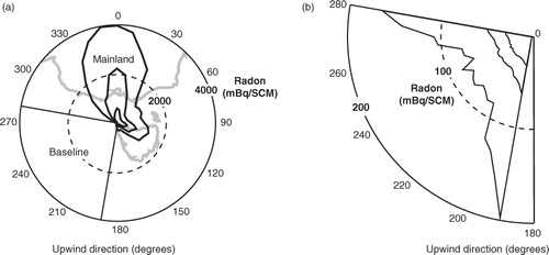
The amplitude of Cape Grim angular radon distributions is dominated by Australian mainland and, to a lesser extent, Tasmanian emissions (Fig. 1a); on a comparable scale baseline radon concentrations appear negligible. This is clearly not the case, however, when the baseline sector is isolated (Fig. 1b). This figure demonstrates not only that baseline radon is measureable, but that its angular distribution within the sector has a distinctive structure (cf. Section 3.1).

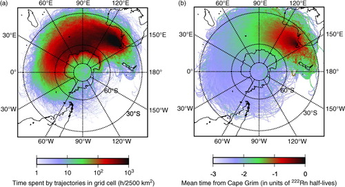
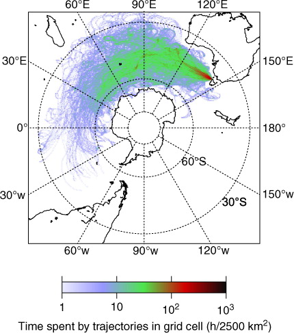
A distinctive characteristic of Cape Grim baseline radon observations is that they are affected by radon emissions over a large geographic area (fetch region). The baseline fetch of the 2001–2008 observations, as delineated by 10-day back trajectories, is shown in Fig. 2a; where density is rendered by a colour contrast signifying the time spent by trajectories in 50×50 km grid cells. The same trajectories are shown in Fig. 2b, only here the colour contrast relates to the mean time required by air parcels moving along trajectories to arrive at Cape Grim. While all fetch regions of Fig. 2b, irrespective of colour, can potentially affect the composition of Cape Grim air parcels, the radon contribution from blue shaded regions, for example, might be reduced by up to 1/8 of its initial value, due to radon's radioactive decay. Notwithstanding the effect of travel time, it is evident that baseline radon observations are affected by air overlying a large portion of the Southern Ocean.

Fig. 2.  2001–2008 back trajectory density functions for all baseline observations at Cape Grim. The density is defined by (a) the time spent by trajectories in 50×50 km grid cells; (b) the mean time required by air parcels moving along trajectories to reach Cape Grim (in units of radon half-lives, T_1/2=3.82 days).

It is evident from Fig. 2 that some baseline air parcels spend considerable time over land masses before arriving at Cape Grim. Given that the oceanic radon flux is significantly smaller than that from land (e.g. Wilkening and Clements, 1975), a considerable overlap between baseline and non-baseline distributions of radon concentrations is to be expected. Quantifying this overlap for the 2001–2008 observations (see Table 1) makes it clear that a considerable portion of the intervening baseline radon observations are significantly influenced by continental emissions.

Table 1. Radon concentration (mBq/SCM) distribution at Cape Grim in 2001–2008 for baseline (local wind direction between 190° and 280°) and non-baseline conditions

	Radon concentration in air (mBq/SCM)
Wind sector	Mean	No. of observations	5th	10th	25th	Median	75th	90th	95th
Baseline	176	28622	8	15	26	42	96	390	850
Non-baseline	976	38799	28	45	121	378	1164	2881	4101

Another fortuitous aspect of baseline observations at Cape Grim is that they occur frequently in all seasons; the percentage of total hourly baseline observations in summer and spring is 27% each, and in winter and autumn is 23% each (cf. Table 2, Set 0). The duration of baseline events typically varies from a few hours to 4 days. The frequency and duration of baseline events are largely controlled by the passage of synoptic-scale weather systems.

Table 2. Radon concentration (mBq/SCM) distributions of baseline observations in composite year and season at Cape Grim in 2001–2008

Radon concentration in air (mBq/SCM)
Set	Season	Mean	No. of observations	5th	10th	25th	median	75th	90th	95th
	Summer	151	7792	4	9	20	34	75	375	808
	Autumn	241	6523	12	18	31	50	149	605	1273
0	Winter	170	6484	16	21	32	46	94	350	731
	Spring	151	7823	7	13	24	40	84	292	651
	All	176	28622	8	15	26	42	96	390	850
R1	All	229	19927	8	16	28	48	152	598	1121
	Summer	31	2401	4	8	16	26	37	54	71
	Autumn	62	2048	11	15	25	39	57	121	203
1	Winter	74	2075	14	21	31	43	61	167	291
	Spring	48	2171	7	11	20	31	53	92	133
	All	53	8695	8	13	22	34	52	91	173
R2	All	60	3416	7	12	21	34	55	114	221
	Summer	29	1473	5	8	16	24	35	52	67
	Autumn	54	1374	12	16	26	39	56	96	171
2	Winter	70	1224	17	23	33	43	59	124	245
	Spring	43	1208	8	12	20	31	51	77	111
	All	48	5279	9	13	22	34	51	79	135
R3	All	194	208	35	48	87	165	241	389	507
	Summer	29	1458	4	8	16	24	35	51	64
	Autumn	48	1299	11	16	25	38	53	71	121
3	Winter	53	1109	17	22	32	41	53	79	118
	Spring	43	1205	8	12	20	31	50	76	111
	All	42	5071	8	13	21	33	48	68	99
R4	All	61	426	4	10	17	33	70	155	201
	Summer	28	1341	5	9	16	25	35	49	61
	Autumn	45	1171	11	15	25	38	51	66	84
4	Winter	52	1047	18	23	32	41	53	73	106
	Spring	40	1086	8	12	20	30	50	72	96
	All	41	4645	9	13	22	33	47	65	85
R5	All	39	988	9	13	23	34	47	63	79
	Summer	29	1170	5	9	16	25	35	49	61
	Autumn	45	903	10	14	24	36	52	67	85
5	Winter	55	751	20	25	33	43	54	77	114
	Spring	41	833	8	12	20	30	50	74	102
	All	41	3657	9	13	21	33	47	66	88
R6	All	38	1267	9	13	20	32	46	65	86
	Summer	28	920	5	9	17	25	35	49	61
	Autumn	46	736	11	15	25	36	51	68	93
6	Winter	61	442	24	27	35	44	55	84	114
	Spring	49	292	7	14	23	37	58	77	117
	All	42	2390	8	13	22	33	48	66	88
R7	All	39	1490	7	12	21	32	47	65	77
	Summer	31	361	9	12	18	27	36	51	62
	Autumn	56	219	14	19	29	40	55	71	212
7	Winter	49	207	25	28	36	44	52	81	104
	Spring	53	113	7	13	22	32	53	100	163
	All	44	900	11	15	23	35	48	66	99

A sequence of concentration sets (from top to bottom) characterises the results of selection steps for obtaining the least perturbed radon concentration set. The sequence starts with the initial baseline observation set defined by the local wind direction only. This is followed by seven sets each of which is obtained by removing some observations from the previous set. Annual distributions of the removed observations (R1–R7) are also shown. See Section 3 for details; bold entries are depicted in Fig. 5.

2.2. Radon measurements: technique and limitations

The measurement technique used to determine hourly atmospheric radon concentrations at Cape Grim is based on the dual flow loop, two-filter method (Whittlestone and Zahorowski, 1998). Since baseline radon concentrations can be 10 mBq m⁻³ or lower (Tables 1 and 2), we have used a large delay volume (5 m³) and multiple, rather than single, sensing head configurations throughout the 2001–2008 period (2, 4 and 8 heads in 2001–2004, 2005– February 2007, March 2007–2008, respectively). The uncertainty associated with hourly radon estimates for concentrations above 70 mBq m⁻³ is less than ±12%; uncertainties are progressively higher for lower concentrations where counting errors begin to dominate. For instance, at 10 mBq m⁻³ the counting error is approximately 40%, and rises to approximately 100% at 4 mBq m⁻³. Calibrations were performed every three to four months until July 2003 and monthly thereafter. Instrumental background was determined sporadically until July 2003, and every 3 months thereafter. Sensing heads have been replaced every 3 years to minimise the accumulation of lead-210 on the second filter. Sampling is conducted from a height of 70 m above ground level (164 m above sea level). The overall recovery rate for hourly radon concentrations over the 8-year period was approximately 96%.

We express all Cape Grim radon concentrations in mBq/SCM, where SCM stands for standard cubic meter; the convention adopted for standard conditions was p=10⁵ Pa and T=213.16 K. Unless otherwise stated, when discussing distributions of radon concentrations we will characterise them by seven percentiles (5th, 10th, 25th, median, 75th, 90th, and 95th), since the often subtle changes discussed do not notably affect means. Means are shown only as required to facilitate comparison with results obtained by other research groups.

3. Least perturbed baseline radon observations

Relating baseline radon observations to radon oceanic flux density can only be done in a straightforward manner for radon concentrations where the corresponding air parcels are in equilibrium with their oceanic radon source. However, as we have previously indicated, a significant fraction of baseline radon observations has been affected (or perturbed) by radon emissions from land. In general, perturbations can be positive or negative, i.e. can lead to higher or lower radon concentrations compared with those in equilibrium with the oceanic radon source. Perturbations of either sign, and the methods leading to identification of baseline observations departing from equilibrium with the oceanic radon source, are discussed in this section. Removal of these observations is achieved in seven steps leading to a final set of least perturbed baseline radon observations.

3.1. Positive perturbations

We begin by identifying baseline observations affected by radon emissions from ice- and snow-free land. Toward the baseline sector boundaries of Fig. 1b the top quartile radon concentrations more than doubles, whereas the median concentrations rise only slightly. To identify and exclude the high-radon air parcels from consideration, we examine baseline events in the time domain in steps 1 and 2 below.

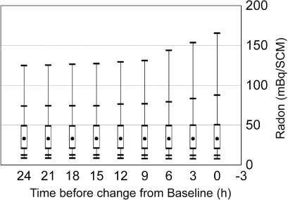
Step 1. Ideally, the distribution of radon concentrations should be examined for consecutive hours (or another suitable period) after change to baseline. However, by doing this considerable scatter occurs in the higher percentiles of events persisting for longer than 40–50 hours, as they are represented by progressively smaller numbers of observations. To avoid this scatter we examine distributions of baseline observations as a function of the minimum length of time they persist in the sector (Fig. 3).

Fig. 3.  Radon concentration (mBq/SCM) distribution characterised by 5th, 10th, 25th, 50th, 75th, 90th, and 95th percentiles in the baseline sector as a function of duration in the baseline sector.

A significant, and consistent, decrease in radon concentrations is evident for baseline observations within the first 12 hours after change to baseline. A less pronounced decrease then continues until 24 hours into baseline conditions, after which time the distribution range reaches a minimum that can be considered a first approximation of least perturbed oceanic air. Based on the above findings, we remove all observations persisting in the baseline sector for less than 24 hours.

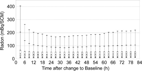
Step 2. For events persisting longer than 36 hours in the sector there is a small widening of radon distributions, mainly due to higher concentrations in the top 10 per cent of observations. This is likely attributable to the fact that at the end of a baseline event, there is an increased likelihood of land radon emissions becoming entrained in the corresponding air parcels that are still nominally baseline. The associated change in air parcel characteristics, such as the observed increase in land perturbation, is gradual. To quantify such perturbations at the end of baseline events we examine radon concentration distributions binned as a function of time until the end of the baseline event (Fig. 4). This figure shows a considerable widening of baseline radon distributions in the last 12 hours that an event spends in the baseline sector. Accordingly, we remove all observations made within the last 12 hours in the baseline sector.

Fig. 4.  Radon concentration (mBq/SCM) distribution characterised by 5th, 10th, 25th, 50th, 75th, 90th, and 95th percentiles in the baseline sector in consecutive 3-hour period before a change to a non-baseline sector.

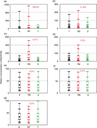
The results of steps 1 and 2, as well as the selections steps that follow, are documented in Fig. 5: each step is represented by a graph showing the radon distributions before and after the selection (left and right distributions, respectively) as well as the distribution of rejected observations (the middle distribution). The graphs also show the number of the rejected events expressed as a percentage of the number of events in the initial baseline set (set 0 in Table 2). Numerical results for each step are also shown in Table 2. Note that the radon distributions of observations rejected in steps 1 and 2 (Fig. 5a and 5b, respectively) are clearly higher than the distributions before and after the respective steps.

Fig. 5.  Radon concentration (mBq/SCM) distributions for the seven selection steps to extract from the initial baseline observations (Set 0 in Table 2) a set of least perturbed radon concentrations in air parcels that are in equilibrium with their oceanic radon source (Set 7 in Table 2). Each step is represented by a graph contrasting a distribution of rejected concentrations (in red) with associated distributions before and after application of the step's selection criterion shown to its left (in black) and right (in green). The number of rejected concentrations expressed as a percentage of the number of events in the initial baseline set (Set 0 in Table 2) is shown in the top right corner. All distributions are identified by their numbers shown in Table 2. Note change of the radon concentration scale between different graphs.

Examination of the events remaining after steps 1 and 2 revealed there were still some high radon observations clearly affected by land emissions. In steps 3 and 4 we identify and exclude these remaining observations using back trajectory analysis.

Step 3. First we removed all observations for which corresponding trajectories indicated any contact with snow- and/or ice-free land (i.e. excluding Antarctica) within 10 days before reaching Cape Grim. Only a limited number of events, 0.7% of the initial set, were directly affected by land. Consequently, although their radon distribution is relatively high (Fig. 5c, middle distribution), the reduction in distribution range is small compared with those in steps 1 and 2 (cf. Fig. 5a and 5b). It is of note, however, that the distribution of observations removed in step 3 is more than twice as wide as that of step 2. This is not surprising as the latter quantifies the changes air parcels undergo while exiting baseline sector, whereas the former deals with changes affected by direct contact with land. The small number of observations rejected in this step is due to the fact that most of the land-affected events were accounted for in steps 1 and 2.

Step 4. We also investigated whether air parcels on their way to Cape Grim may have had their radon concentration affected by mixing with off-shore radon-rich air. The strength and geographical extent of land influence on offshore radon concentrations is best quantified directly by ship radon transects. We addressed the current lack of suitable ship transects in our study domain by investigating how close air parcels travelled to the southern shore of the Australian mainland. We assumed that this region is most likely to contribute to the effect based on the prevailing airflow in the baseline sector (cf. Fig. 2a and 2b). We estimated the magnitude of the effect by identifying baseline trajectories traversing within 2° latitude of the Australian coast and analysing the radon distributions of observations that mixed progressively less with the radon-rich offshore air, as determined by the number of hours in the last 10 days the corresponding trajectories spent in that band. We found a discernible effect of this mixing in that the change is most pronounced in autumn and negligible in summer. In autumn, the mixing affects the top 5% of observations by reducing the 95th percentile from 121 mBq/SCM to 84 mBq/SCM (Sets 3 and 4 in Table 2). Similar to the previous step, the number of the rejected observations is small (1.5% of the initial baseline set) and the distribution of the rejected concentrations significantly wider (the middle distribution in Fig. 5d and Set R4 in Table 2) and comparable to that of Step 2.

The above four steps combined led to a 10, 6, and 2 times reduction of the 95th, 90th, and 75th percentiles of the annual distribution, respectively. Note, however, that the overall reduction in the median is only 20% (Table 2).

3.2. Negative perturbations

We now examine effects that can potentially result in negative perturbations of observed baseline radon concentrations. The first two relate to an air parcel's radon composition being affected by contact with land covered with snow and/or ice sheets (Step 5), or by contact with ice-covered ocean (Step 6). Such covers (full or partial), will lead to suppression of radon emissions and possibly lead to radon flux densities discernibly lower than those that are characteristic for ice-free ocean. Any extended period spent over such surfaces might lead to lower radon concentrations observed at Cape Grim.

Step 5. We identified snow/ice affected baseline observations by selecting events for which corresponding air parcels traversed Antarctica. The distribution of the excluded observations is discernibly lower than of the input set (R5 in Fig. 5e), even though air parcels affected by passage over Antarctica then spent considerable time above the ocean before arriving at Cape Grim; during that passage, concentrations can be reduced by 4–8 times (cf. Fig. 2b). Note that the observed effect might also be due to the passage of air parcels over ice-covered sea.

Step 6. We found more than 1200 observations (cf. Table 2) for which trajectories had not traversed Antarctica, but were over ice-covered sea (Stroeve and Meier, 2012). Removing these observations had a very small effect on the spring radon distributions, which was the season most represented in the removed set (cf. Sets 5 and 6 in Table 2).

Step 7. In the final step, we attempted to account for dilution of marine boundary layer radon by free tropospheric air, due to large scale air movements across the top of the boundary layer. Such dilution is possible due to the relatively short half-life of radon, resulting in a radon concentration gradient across the top of the marine boundary layer (e.g. Kritz et al., 1998; Williams et al., 2011).

To account for such events we excluded observations corresponding to air parcels that spent more than 30% of the 10 days before arrival at Cape Grim in the free troposphere. The overall effect of this exclusion leads to a non-negligible upward shift of the distribution (Fig. 5g and Table 2), irrespective of season (not shown). Imposing any further restriction on the time trajectories spent within the Marine Boundary Layer (MBL) drastically reduces the number of observations with a negligible impact on the resulting radon distribution.

In order to exclude trajectories that had limited contact with the ocean surface before arriving at Cape Grim, we defined the weighted fractional time inside the MBL. For a trajectory s , starting at time t ₀ and terminating at Cape Grim at time T, the weighted fractional time inside the MBL, T _MBL, is:1

where I(s,t)=1 if s is inside the boundary layer at time t, and 0 otherwise. λ=2.0982×10⁻⁶ s⁻¹ is the decay constant of radon–222, and τ is the decay timescale associated with the entire (finite) trajectory. Note that for non-decaying species (λ=0), τ=T−t ₀.

We postulate that the final set (Set 7 in Table 2, and Fig. 6, showing the final set's trajectories), obtained after application of the seven selection steps, constitutes the least perturbed baseline radon observations at Cape Grim for the 2001–2008 period. Accordingly, we use this set below for estimating the oceanic radon flux. Note that the process of eliminating perturbed observations also results in a drastic reduction of available observations after each step as shown in Fig. 5 and Table 2.

Fig. 6.  2001–2008 back trajectory density functions for least perturbed baseline observations (Set 7 in Table 2) at Cape Grim. The density is defined by the time spent by trajectories in 50×50 km grid cells.

4. Estimation of radon flux density

Having identified a least perturbed set of radon concentrations, we now derive an expression for the mean oceanic radon flux as a function of the radon concentrations (Section 4.1), and define other variables required for the final flux calculation (Sections 4.2 and 4.3).

4.1. Estimation of the flux

The vertically integrated boundary layer radon budget following an air parcel trajectory can be written as:2

where R is the total radon per unit area in the boundary layer, h is boundary layer depth, c(z) is radon concentration at height z, and F is the net radon flux density into the column. For a trajectory starting at time t ₀ and terminating at the point of interest at time T, Equation 2 has the solution:3

where R ₀ =R(t ₀ ) and is an exponentially weighted mean flux:4

For an infinite trajectory, (T−t ₀ )→∞ and . Expressing as a balance between the mean oceanic radon flux F _ocean and a venting flux out of the boundary layer top F _vent , we then obtain from Equation 3:5

Assuming radon is uniformly distributed with height throughout the boundary layer, we set , the atmospheric radon concentration measured near the surface. Further assuming significantly lower radon above the boundary layer (Kritz et al., 1998; Williams et al., 2011), we can parameterise the venting flux as:6

where w _e is the entrainment velocity and is the concentration jump across the boundary layer top. Substitution into Equation 5 produces an expression for the mean oceanic radon flux:7

We use Equation 7 for oceanic radon flux estimates, substituting for c _sfce hourly baseline radon observations from the least perturbed oceanic set defined in the previous section. As a result, we obtain a range of flux estimates reflecting a range of conditions in the 2001–2008 period. Estimates of the other two variables in Equation 7, the entrainment velocity w _e and mixing height h are discussed below.

4.2. Mixing height at Cape Grim

We used data from the ERA-Interim reanalysis (Simmons et al., 2007), to estimate mixing depths at Cape Grim during each of the least perturbed baseline events in 2001–2008. The reanalysis model is based on the European Centre for Medium-Range Weather Forecasts (ECMWF) operational model, and provides mixing depth output on a 1.5° grid every 3 hours based on a Richardson Number definition of PBL (Palm et al., 2005). Data were taken from the nearest oceanic grid point to Cape Grim, located at 40.5°S, 144°E.

The mixing height from various implementations of this model has been compared with radio-sonde and satellite observations, generally with encouraging results:

• A bias in mixing height of approximately 20 m (model too low by 2 hPa), with RMS error of 200 m, was reported by von Engeln et al. (2003) from 86 radio-sonde ascents launched from 10 island stations, including Amsterdam Island at a similar latitude to Cape Grim but 5,600 km upwind.

• The earlier ERA-15 reanalysis captured the thermal structure of the boundary layer near 31°N, but cloud cover was strongly underestimated; observed low cloud cover was 83% compared with the modelled 22% (Duynkerke and Teixeira, 2001).

• Model mixing heights compared well to multi-year mean mixing height from radio occultation-derived mixing heights (von Engeln et al., 2005). Compared with the GLAS satellite lidar, however, the mixing height in the ECMWF model was an average of 200–400 m lower, although it exhibited similar spatial patterns along satellite tracks (Palm et al., 2005).

Given the above, there was a reason to test the validity of the modelled mixing heights near Cape Grim. We achieved this by comparing model output to mixing heights derived from the Mini-Lidar data gathered at Cape Grim during the second half of 1998 (Young, 2006, 2007). Sixteen baseline events were selected from June to December 1998 for the comparison. Low clouds prevailed during these events, consistent with the cloud climatology of this region (Warren et al., 1988).

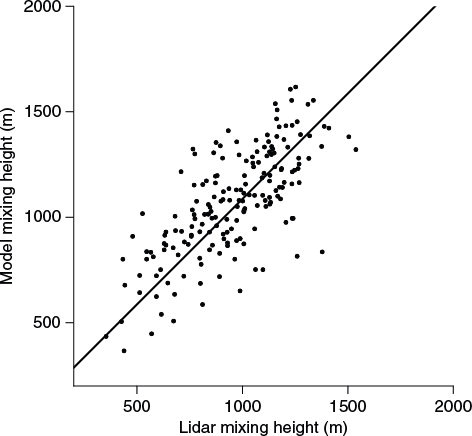
To derive mixing heights from the lidar data, the mixing height was taken to be the top of the lowest cloud layer. This height was determined manually, as the low signal-to-noise ratio of the lidar makes alternatives impractical. As a consequence of the method, the determination of mixing height was partly subjective, and becomes more so during periods of ambiguous lidar signals. The analysis method also suffers from the inability to detect a decoupled boundary layer beneath low cloud. Nevertheless, lidar and model mixing heights agree well (Fig. 7). Based on 183 lidar measurements of mixing height, the lidar-derived mean mixing height of 956 m is approximately 11% lower than the ERA-Interim mixing height of 1069 m, with an RMS error of 217 m.

Fig. 7.  ERA-Interim mixing height (labelled model) at the closest oceanic grid point to Cape Grim compared with mini-lidar mixing height measurements at Cape Grim during 14 baseline events in 1998. An orthogonal distance regression fitting line (slope 1.03) shown on the scatter plot explains 85% of the variance.

4.3. Entrainment velocity

For mid-latitudes, the marine boundary layer is typically shallower than its terrestrial counterpart and exhibits limited diurnal variability (e.g. Kritz, 1983). The primary capping inversion that separates MBL processes from the free troposphere is usually found 1000–1900 m above sea level (Ayers and Galbally, 1995; Boers et al., 1998; Russell et al., 1998; Lenschow et al., 1999). When present, cloud base usually lies between 400 and 800 m, and the overlying cloud layer is often less than 500 m thick (Russell et al., 1998; Lenschow et al., 1999). Depending on local meteorological conditions, a secondary inversion may form at – or near – cloud base, resulting in the formation of a detached buffer layer between MBL processes and the free troposphere (Russell et al., 1998).

To a first approximation, the mid-latitude MBL is often assumed to be capped by an impermeable temperature inversion (e.g. Raes, 1995). There is, however, an exchange mechanism (entrainment) that links MBL processes and products to the free troposphere, and vice versa, which plays an important role in cloud formation as well as the budgets of aerosols and trace gas species (Moeng et al., 1996; Lenschow et al., 1999; Osborne et al., 2000; Sollazzo et al., 2000). MBL entrainment/detrainment is contributed to by two processes: (1) cloud venting processes (e.g. Cotton et al., 1995), and (2) the balance between large scale subsidence and changes in mixing depth (Kritz, 1983).

Mid latitude MBL entrainment rates, with the exception of isolated cases (e.g. −30 to 50 mm s⁻¹, Sollazzo et al., 2000; 6–12 mm s⁻¹, Wang et al., 2008), are generally found to be between 0 and 10 mm s⁻¹ (Boers and Betts, 1988; Russell et al., 1998; Lenschow et al., 1999; Wang et al., 1999b; Yi et al., 2008). Estimates within this range include 6.5 mm s⁻¹ (Bretherton et al., 1995; Sollazzo et al., 2000), 3–6 mm s⁻¹ (Raes, 1995; Clarke et al., 1996) and 0–5 mm s⁻¹ (Kawa and Pearson, 1989; De Roode and Duynkerke, 1997; Wang et al., 1999a; Hill et al., 2008; Faloona, 2009; Lock, 2009). The most common estimate for mid-latitude MBL entrainment for clear and cloudy conditions, however, is 3–4 mm s⁻¹ (e.g. Kritz, 1983; Ayers and Galbally, 1995; Boers et al., 1998; Stevens et al., 2003; Sandu et al., 2009). In most cases, the uncertainty associated with these estimates is of the order of 25–60%.

Taking into account the abovementioned published data and assuming that fairly uniform meteorological conditions prevailed during the baseline events of the least perturbed set, we have adopted a constant entrainment rate of 4 mm s⁻¹ and assumed a conservative uncertainty of 50%.

5. Results and discussion

Annual and seasonal distributions of the oceanic radon flux density are summarised in the top section of Table 3. We start the discussion by comparing our flux results with those obtained by other researchers either from spot measurements, or model estimates; commonly assumed oceanic flux for comparisons of regional or global models are also included.

Table 3. Comparison of oceanic radon flux densities (mBq m⁻² s⁻¹) obtained in this paper (top section of the table) followed by spot measurements (accumulator and profile techniques), modelled flux, and assumed in or inferred from general circulation models

			Radon-222 flux density (mBq m^−2 s^−1)			Wind speed (m s^−1)
Source	Method	Region	10th/50th/90th percentiles	Mean and standard deviation	No. of samples	Mean and standard deviation Range 10th/50th/90th percentiles
			Summer	0.190±0.122	361	12.2/15.2/19.9^a
			0.071/0.164/0.311
			Autumn	0.347±0.37	219	11.0/15.0/21.0^a
			0.109/0.273/0.513
This study	Radon concentrations in boundary layer air at costal site	Southern Ocean	Winter	0.303±0.17	207	12.6/16.5/22.0^a
			0.167/0.267/0.508
			Spring	0.318±0.39	113	11.1/15.3/18.8^a
			0.081/0.202/0.631
			All seasons	0.270±0.261	900	12.1/15.7/20.7^a
			0.092/0.218/0.429
Flux spot measurements
Wilkening and Clements, 1975	Accumulator	Tropical Pacific		0.16±0.02	Not reported	3
Duenas et al., 1983	Accumulator	West Mediterranean	0.05/0.11/0.30	0.14±0.09	36	0.5/2.6/5.6
Broecker and Peng, 1971	Radon profiles	North Atlantic trade wind belt	0.021/0.024/0.029	0.024±0.0031	45	5–7.5
Hoang and Servant, 1972	Radon profiles	Southern Ocean		0.24±0.15	12	6.6±4.3
Peng et al., 1974	Radon profiles	North Pacific		0.08±0.03	7	8.9±3.0
Peng et al., 1979	Radon profiles	South Atlantic^b		0.04±0.02	9	7.8±3.3
Smethie et al., 1985	Radon profiles	Tropical Atlantic	0.05/0.15/0.30	0.17±0.12	29	4.9/7.1/10.0
Kawabata et al., 2003	Radon profiles	West North Pacific		0.12±0.08	13	15.7±7.5
Flux model
Schery and Huang, 2004	Flux model	Southern Ocean^c	0.04/0.06/0.08	0.06±0.02	n/a	n/a
Flux assumed for or inferred from models
Jacob et al., 1997	Model	All oceans, 60°N–60°S	0.11			n/a
Mahowald et al., 1997	Model	Southern Ocean	0.06			n/a
Schery and Wasiolek, 1998	Model	All oceans and ice covered regions	0.14			n/a
Taguchi et al., 2002	Model	All oceans, 60°N–60°S	0.21			n/a
Law et al., 2008	Model	All oceans, 70°N–70°S	0.11			n/a

^aDistribution of trajectory averaged wind speeds weighted by radon decay.

^bNine samples from the Southern Atlantic – the study reports 100 measurements.

^cGlobal model, results shown in the table refer to the Southern Ocean only.

5.1. Comparison of oceanic fluxes with other estimates

Over the past four decades, a number of attempts have been made to experimentally constrain the magnitude of the radon flux density for different oceanic regions. These attempts are summarised in Table 3. The experimental techniques used for the estimates were: (1) direct measurement using accumulation chambers (cf. Wilkening and Clements, 1975; Dueñas et al., 1983); and (2) using vertical profiles of oceanic ²²⁶Ra/²²²Rn to infer radon flux to the atmosphere (Hoang and Servant, 1972; Peng et al., 1974; Smethie et al., 1985; Kawabata et al., 2003). The means range from 0.024 mBq m⁻² s⁻¹ (Broecker and Peng, 1974) to 0.24 mBq m⁻² s⁻¹ (Hoang and Servant, 1972).

Of the eight experimental estimates of the oceanic radon flux density shown in Table 3, only one study (Hoang and Servant, 1972) specifically targeted the Southern Ocean. Only 12 spot measurements were made with a mean equal to 0.24±0.15 mBq m⁻² s⁻¹. The radium profiles on which the results of Hoang and Servant (1972) were based were collected in two cruises that spanned the latitudes 38°10′S to 66°14′S of the Southern Ocean (Ku et al., 1970). The northernmost profiles were conducted in August–September and the southernmost in January–February.

The mean radon flux density derived from this study is equal to 0.270±0.261 mBq m⁻² s⁻¹, which agrees well with the mean proposed by Hoang and Servant. The agreement should be viewed with some caution. Firstly, we compare the means of a small number of spot flux density measurements with an average of a large number of estimates representing large oceanic areas (cf. Table 3). Secondly, the flux densities we calculate have their own, significant uncertainty. The most important factor contributing to that uncertainty is the uncertainty associated with entrainment velocity. We have adopted a constant entrainment rate of 4 mm s⁻¹ and have assumed a conservative uncertainty of 50% (Section 4.3). Hence, at least the same uncertainty has to be attributed to radon flux density distributions (cf. Equation 7). Constraining such an uncertainty could be one of the most effective future refinements of our results once better constrained and possibly time dependent entrainment velocity estimates become available. By contrast, uncertainty due to mixing height at Cape Grim, interpolated from the ERA-Interim reanalysis for each hourly event in the least perturbed set is significantly smaller (a bias of 11%, Section 4.2) and can be neglected in view of the entrainment velocity uncertainty.

Another possible refinement of our radon flux densities could result from a reanalysis of the underlying baseline observations using a multi-particle (e.g. Arnold et al., 2010) rather than single-particle method for generation of back-trajectories. We think that such a refinement is possible, and would have the advantage that dispersion and turbulent mixing processes would be included, but whether it would result in a significant change of our results is less certain. Firstly, despite the error from modelling air mass back-trajectories as single particles (Stohl et al., 2002), we attribute fluxes to a very large source region, employ conservative data selection rules, and base results on a large number of trajectories, all of which allows our method to tolerate a large uncertainty in the position of individual back-trajectories. Secondly, any benefit of eliminating this error would be reduced by the relative scarcity of meteorological data in our study domain. And thirdly, uncertainties of 10-day back-trajectories are relatively large regardless of the method employed for their generation – see for instance Draxler (1991); Engström and Magnusson (2009) and Wen et al. (2012) for experimental and numerical treatment of the uncertainties associated with back-trajectories.

Considerable seasonal variability was observed in the median oceanic radon flux density estimate, from 0.164 mBq m⁻² s⁻¹ in summer to 0.267 mBq m⁻² s⁻¹ in winter. The mean flux density estimate based on our summer observations (0.19±0.12 mBq m⁻² s⁻¹) compares well with flux densities reported from the tropical Pacific (0.16±0.02 mBq m⁻² s⁻¹; Wilkening and Clements, 1975) and the tropical Atlantic (0.17 mBq m⁻² s⁻¹; Smethie et al., 1985).

However, a number of other experimentally estimated flux densities (Table 3) were considerably lower than values reported in this study. The nature of accumulation measurements of the oceanic radon flux biases results toward low wind speed/wave height conditions. Similarly, the challenges involved in making ship-based profile measurements in conditions of high seas result in a low-to-medium wind speed bias on such results. These biases may explain why many of the existing experimental estimates of the oceanic radon flux density are lower than those reported here. Hence, it is possibly not a coincidence that the two studies that reported making radium profile observations under conditions of higher wind speeds (Peng et al., 1974; Kawabata et al., 2003), reported the upper boundaries of their radon flux density results at 0.12 and 0.23 mBq m⁻² s⁻¹, respectively (Table 3), which are closer to the findings of this study.

Southern Ocean specific radon flux densities that have been inferred from modelling studies: 0.06 mBq m⁻² s⁻¹ (Mahowald et al., 1997), 0.06 mBq m⁻² s⁻¹ (Schery and Huang, 2004) are more than four times lower than our mean radon flux density. Of the oceanic flux density assumed for modelling studies, the ones closer to this study are those of Taguchi et al. (2002) (0.21 mBq m⁻² s⁻¹) and Schery and Wasiolek (1998) (0.14 mBq m⁻² s⁻¹).

5.2. Dependence on wind speed, significant wave height, and latitude

Having established a significant number of hourly estimates of oceanic radon flux, we are now equipped to look for a relationship between these radon emissions and other quantities that we can estimate along a trajectory. In practice, any relationship will be overwhelmed by noise unless the quantity under investigation varies smoothly compared with the uncertainty in trajectory position. We start with wind speed, which is known to have a strong effect on ocean–atmosphere gas exchange (Wanninkhof, 1992; Nightingale et al., 2000; McGillis et al., 2004; McNeil and D'Asaro, 2007; Jeffery et al., 2008).

In an attempt to consider only the most accurate trajectories, we exclude points within 4 hours of the start or end of a least-perturbed baseline event, based on the premise that trajectories will be more accurate under steady conditions (Stohl, 1998). We compute wind speed from the hourly distance travelled by trajectories and then compute an average along the trajectory after weighting each point by the radon decay fraction. A plot of calculated flux vs. wind speed is shown in Fig. 8a.

Fig. 8.  Oceanic radon flux density (mBq m⁻² s⁻¹) as a function of: (a) radon weighted trajectory mean wind speed (0.6 m s⁻¹ bins), and (b) significant wave height (0.15 m bins). Whiskers show the quartile range of the radon flux density with crosses indicating the bin median and dots the bin mean. Solid lines represent a quadratic fit a*x²+c. Coefficients (variance) of the fit are for (a) a=0.000580 (1.0293*10⁻⁸), c=0.0682 (0.000721), and for (b) a=0.017 (2.798*10⁻⁶), c=0.00679 (0.000534).

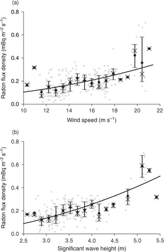
As it is a more smoothly varying field, and because sea state has also been shown to affect gas exchange (Woolf, 2005), we perform the same analysis using significant wave height, extracted from the ERA-Interim Reanalysis (Simmons et al., 2007). The reanalysis data shows that the significant wave height within the Southern Ocean fetch region of this study approximately doubles from summer to winter. When distributions of radon flux density estimates were calculated for 0.2 m wave height bins, a clear relationship emerged (Fig. 8b). This result is consistent with numerous investigations into the effects of waves and bubble-action on rates of air–sea trace gas exchange (D'Asaro and McNeil, 2007; Fangohr and Woolf, 2007; Rhee et al., 2007; Woolf et al., 2007; Tsoukala and Moutzouris, 2008).

In both cases a quadratic fit is consistent with observations, notwithstanding a small number of samples in the lowest and highest bins. This can be seen as an independent argument in support of our assumption that the flux estimates we made based on the least perturbed set are indeed representative of an actual oceanic flux, and that the least perturbed radon concentration set (Table 2, Set 7) air parcels are in equilibrium with the oceanic radon source.

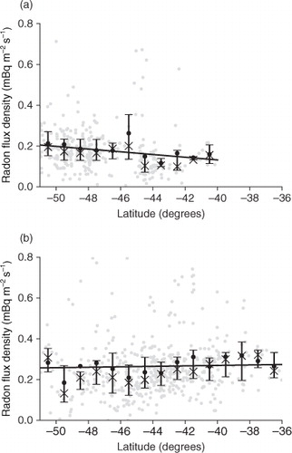
To investigate the possibility of latitudinal dependence, we grouped the radon flux density estimates according to the average latitude of the corresponding trajectories weighted by radon decay (Fig. 9). In summer months (representing 40% of all observations), radon flux densities in 1° latitude bins increased southward of 40°S to a maximum value between 52 and 54°S (Fig. 9a). This result is consistent with a similar increase, in summer, in Southern Hemisphere zonal mean wind speed (based on the ERA-Interim data) from 30 to 52°S (not shown). In non-summer months (60% of observations), however, radon flux density estimates displayed no significant dependency on latitude (Fig. 9b). This is despite the fact that the corresponding relationship between trajectory speed and latitude shows an increase in speed towards the pole (0.25 ms⁻¹/degree).

Fig. 9.  Oceanic radon flux density (mBq m⁻² s⁻¹) as a function of latitude (1° bins) for (a) summer and (b) non-summer months. Whiskers show the quartile range of the radon flux density with crosses indicating the bin median and dots the bin mean. Solid lines represent a linear fit. Coefficients of the fit are: (a) slope= −0.00667, intercept=0.135; correlation coefficient=−0.176, significance level=99.9%, and (b) slope= 0.00111, intercept= 0.314, correlation coefficient=0.034, significance level=55.3%.

5.3. Distribution of oceanic radon flux density

We note that the flux range derived from the selected radon hourly observations, as has been done in this study, arises from a combination (or convolution) of variability in the oceanic emissions, and the effects of transport and mixing. Mixing processes, which affect the composition of air parcels, are not taken into account by our trajectory-based analysis.

We attempted to isolate the effect of processes other than flux variability on the radon flux distribution by comparing our radon concentration with output from several transport models, which have all proscribed constant oceanic radon fluxes. We chose to compare experimental and model concentrations, rather than the corresponding fluxes, as the experimental concentrations are measured directly.

For this purpose, we used TransCom results for the 2002–2003 period (Law et al., 2008), selecting only those hours (327) that were coincident with the Southern Ocean selected hours from the observations (Set 7). This assumes that the transport is sufficiently well modelled that the temporal selection is filtering the model data in the same way as the observations. Examination of the model time series suggests that this is true, with only 1 hour when all models exceed the observed concentration by>100 mBq m⁻² s⁻¹. Since model radon concentrations were obtained using a single proscribed oceanic flux (0.11 mBq m⁻² s⁻¹), broadening of the models’ radon concentration distributions should be entirely attributable to their transport and mixing processes. We obtain an estimate of the radon flux variability by determining how much more the modelled distributions need to be broadened (by convolution with a normal or log-normal distribution) in order to match observations.

Our initial selection of TransCom model output followed that proposed by Law et al. (2010), whose choice was based on a criterion of how well the models differentiated between baseline and non-baseline periods at Cape Grim (see Law et al., 2010 for details justifying the selection; the list of selected models is in their Table 1). We further refined the selection by requiring the models’ median radon concentrations to be within the 5th–95th percentile range of our experimental radon concentration distribution. This is important since the model's distribution tends to scale with the model's median value so models with poorly simulated median values could bias the assessment of distribution broadening. Seven models fulfilled the condition. Experimental and model-average radon concentration distributions are shown in Fig. 10. Contributing model distributions are also shown to illustrate the differences between the selected models.

Fig. 10.  Comparison of radon concentration (mBq/SCM; relative to the median) distributions for the least perturbed set in 2002–2003 obtained from experiment (E) and averaged model (M); the contributing models’ distributions are also shown (1=AM2.GFDL; 2=AM2t.GFDL; 3=CCAM.CSIRO; 4=CCSR_NIES1.FRCGC; 5=CCSR_NIES2.FRCGC; 6=PCTM.CSU; 7=TM3_vfg.BGC). For details regarding the models see Law et al., 2008, 2010.

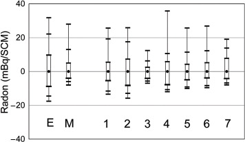
Based on the experimental and model-average distributions in Fig. 10, we estimated the required model-average distribution broadening to best match the experimental distribution, using both normal and lognormal functions. We found the former led to a far better fit with the experiment; the RMS of residuals was 0.032 and 0.094 for the normal (σ=11.3 mBq m⁻³) and log-normal (σ=0.81 mBq m⁻³) broadening functions, respectively; RMS is expressed as a fraction of the maximum frequency of the experimental distribution. Based on this result we postulate that the variability of the oceanic radon flux density, integrated and weighted by radon decay along trajectories, can be approximated by a normal distribution with σ= 0.075 mBq m⁻² s⁻¹.

6. Conclusions

We have addressed the problem of representativeness of spot measurements of oceanic radon flux densities, as well as their scarcity and associated logistic and resource problems, by proposing and testing an experimental method for constraining radon flux density averaged over large oceanic regions. The method was based on hourly radon concentrations measured in marine air at Cape Grim, a coastal baseline site, over the period 2001–2008. The concentrations are selected to represent air parcels least perturbed by land emissions and dilution by the free troposphere, so that they can be assumed to be in equilibrium with the oceanic radon source. The calculated radon flux density distribution is representative for large areas of the Southern Ocean, an important fetch area for climate and air pollution studies in the Southern Hemisphere.

The result compares well with the few available spot measurements of radon flux density from the Southern Ocean. Our flux estimates are close to some spot measurements made in other oceanic regions; in some cases, however, our results are significantly higher. We can only assume that some spot measurements were made in calm sea conditions and thus they tend to underestimate the actual average flux density. In addition, our flux density mean is significantly higher than most of those assumed for modelling studies and for model comparison.

The obtained radon flux density estimates show a significant seasonal dependence and, in summer, a latitudinal dependence which has previously been independently postulated. The flux density also depends on wind speed and significant wave height. In both cases, this is consistent with a quadratic dependence, as is the gas exchange coefficient. The observed quadratic dependence validates our choice of least perturbed concentrations as being in equilibrium with the oceanic radon source.

We emphasise that the radon flux density distribution we obtained should be interpreted as a distribution that constrains the, likely narrower, actual flux distribution. This is due to the fact that least perturbed radon concentration distributions are broadened not only by the corresponding flux variability but also by a number of mechanisms which air parcels are subjected to before arriving at the measurement site. By comparing the least perturbed radon concentration distribution obtained in this study with a corresponding distribution of modelled hourly observations averaged from seven TransCom models that all approximate the oceanic radon flux by a constant, the best agreement between the two is for a normally distributed oceanic flux with σ=0.075 mBq m⁻² s⁻¹.

In future, a similar method could be applied to more remote measurements with less land influence, such as those we recently commenced at Macquarie Island, to further constrain or confirm these estimates.

Acknowledgements

We thank the staff at the Cape Grim Baseline Air Pollution Station in Tasmania as well as Ot Sisoutham and Adrian Element at Australian Nuclear Science and Technology Organisation for their support of the radon measurement program at Cape Grim and Stuart Young and Graeme Patterson for acquiring and pre-processing lidar data at Cape Grim. We acknowledge the NOAA Air Resources Laboratory (ARL) who made available the HYSPLIT transport and dispersion model and the relevant input files for the generation of back-trajectories used in this paper. ECMWF ERA-Interim and sea ice data used in this study were obtained from the ECMWF and NSIDC data servers, respectively. The TransCom model simulations were provided by AM2/AM2t (S. Fan, S.-J. Lin), CCAM (R. M. Law), CCSR_NIES1/2 (P. Patra, M. Takigawa), PCTM.CSU (R. Lokupitiya, A. S. Denning, N. Parazoo, J. Kleist), TM3_vfg (C. Rödenbeck). Instructions for accessing the model output can be found at http://transcom.project.asu.edu/T4_continuousSim.php. One of us (WZ) is indebted to Stewart Whittlestone for an introduction to the field of radon baseline observations.

References

- Arnold D, Vargas A, Vermeulen A. T, Verheggen B, Seibert P. Analysis of radon origin by backward atmospheric transport modelling. Atmos. Environ. 2010; 44: 494–502. 10.3402/tellusb.v65i0.19622.
- Ayers, G. P and Galbally, I. E. 1995. A preliminary estimation of a boundary layer – free troposphere entrainment velocity at Cape Grim. In: Baseline Atmospheric Program Australia 1992. A. L.Dick and P. J.Fraser. Australian Bureau of Meteorology and CSIRO Division of Atmospheric Research, Melbourne. pp. 10–15.
- Boers R, Betts A. K. Saturation point structure of marine stratocumulus clouds. J. Atmos. Sci. 1988; 45: 1156–1175.
- Boers R, Krummel P. B, Siems S. T, Hess G. D. Thermodynamic structure and entrainment of stratocumulus over the Southern Ocean. J. Geophys. Res. 1998; 103(D13): 16637–16650. 10.3402/tellusb.v65i0.19622.
- Bretherton C. S, Austin P, Siems S. T. Cloudiness and marine boundary layer dynamics in the ASTEX Lagrangian experiments. Part II: cloudiness, drizzle, surface fluxes, and entrainment. J. Atmos. Sci. 1995; 52(16): 2724–2735.
- Broecker W. S, Peng T.-H. The vertical distribution of radon in the BOMEX area. Earth. Planet. Sci. Lett. 1971; 11: 99–108. 10.3402/tellusb.v65i0.19622.
- Broecker W. S, Peng T.-H. Gas exchange rates between air and sea. Tellus. 1974; 24(1–2): 21–35.
- Clarke A. D, Uehara T, Porter J. N. Lagrangian evolution of an aerosol during the Atlantic stratocumulus transition experiment. J. Geophys. Res. 1996; 101(D2): 4351–4362. 10.3402/tellusb.v65i0.19622.
- Conen F, Robertson L. Latitudinal distribution of radon-222 flux from continents. Tellus. B. 2002; 54(2): 127–133. 10.3402/tellusb.v65i0.19622.
- Cotton, W. R, Alexander, G. D, Hertenstein, R, Walko, R. L, McAnelly, R. L. and co-authors. 1995. Cloud venting—a review and some new global annual estimates. Earth-Sci. Rev. 39: 169–206. 10.3402/tellusb.v65i0.19622.
- D'Asaro E, McNeil C. Air—sea gas exchange at extreme wind speeds measured by autonomous oceanographic floats. J. Mar. Syst. 2007; 66(1–4): 92–109. 10.3402/tellusb.v65i0.19622.
- Dentener F, Feichter J, Jeuken A. Simulation of the transport of Rn222 using on-line and offline global models at different horizontal resolutions: a detailed comparison with measurements. Tellus. B. 1999; 51: 573–602. 10.3402/tellusb.v65i0.19622.
- De Roode S. R, Duynkerke R. G. Observed Lagrangian transition of stratocumulus into cumulus during ASTEX: mean state and turbulence structure. J. Atmos. Sci. 1997; 54(17): 2157–2173.
- Draxler R. R. The accuracy of trajectories during ANATEX calculated using dynamic model analysis versus raw in sonde observations. J. Appl. Meteorol. 1991; 30: 1466–1467.
- Dueñas C, Fernández M. C, Martinez M. P. Radon from the ocean surface. J. Geophys. Res. 1983; 88(C13): 8613–8616. 10.3402/tellusb.v65i0.19622.
- Duynkerke P. G, Teixeira J. Comparison of the ECMWF reanalysis with FIRE I observations: diurnal variation of marine stratocumulus. J. Clim. 2001; 14(7): 1466–1478.
- Engström A, Magnusson L. Estimating trajectory uncertainties due to flow dependent error in the atmospheric analysis. Atmos. Chem. Phys. 2009; 9: 8857–8867. 10.3402/tellusb.v65i0.19622.
- Faloona I. Sulfur processing in the marine atmospheric boundary layer: a review and critical assessment of modeling uncertainties. Atmos. Environ. 2009; 43(18): 2841–2854. 10.3402/tellusb.v65i0.19622.
- Fangohr S, Woolf D. K. Application of new parameterizations of gas transfer velocity and their impact on regional and global marine CO2 budgets. J. Mar. Syst. 2007; 66: 195–203. 10.3402/tellusb.v65i0.19622.
- Goto, M, Moriizumi, J.,Yamazawa, H, Iida, T and Zhuo, W. 2008. Estimation of global radon exhalation rate distribution. In: The Natural Radiation Environment, 8th International Symposium (NRE VIII). A. S.Paschoa and S.Friedrich Vol. 1034, American Institute of Physics Conference Proceedings, Melville, New York. pp. 169–172.
- Griffiths A. D, Zahorowski W, Element A, Werczynski S. A map of radon flux at the Australian land surface. Atmos. Chem. Phys. 2010; 10: 8969–8982. 10.3402/tellusb.v65i0.19622.
- Hill A. A, Dobbie S, Yin Y. The impact of aerosols on non-precipitating marine stratocumulus. I: model description and prediction of the indirect effect. Q. J. Roy. Meteorol. Soc. 2008; 134(634): 1143–1154. 10.3402/tellusb.v65i0.19622.
- Hoang C.-T, Servant J. Radon flux from the sea (in French). C. R. Acad. Sci. Paris. 1972; 274: 3157–3160.
- Jacob D. J, Prather M. J. Radon-222 as a test of convective transport in a general circulation model. Tellus. B. 1990; 42: 118–134. 10.3402/tellusb.v65i0.19622.
- Jacob, D, Prather, M, Rasch, P, Shia, R, Balkanski, Y. and co-authors. 1997. Evaluation and intercomparison of global atmospheric transport models using 222Rn and other short-lived tracers. J. Geophys. Res. 102: 5953–5970. 10.3402/tellusb.v65i0.19622.
- Jeffery C. D, Robinson I. S, Woolf D. K, Donlon C. J. The response to phase-dependent wind stress and cloud fraction of the diurnal cycle of SST and air–sea CO2 exchange. Ocean. Model. 2008; 23: 33–48. 10.3402/tellusb.v65i0.19622.
- Kawabata H, Narita H, Harada K, Tsunogai S, Kusakabe M. Air—sea gas transfer velocity in stormy winter estimated from radon deficiency. J. Oceanogr. 2003; 59: 651–661. 10.3402/tellusb.v65i0.19622.
- Kawa S. R, Pearson R. J. An observational study of stratocumulus entrainment and thermodynamics. J. Atmos. Sci. 1989; 46(17): 2649–2661.
- Kritz M. A. Use of long-lived radon daughters as indicators of exchange between the free troposphere and the marine boundary layer. J. Geophys. Res. 1983; 88(C13): 8569–8573. 10.3402/tellusb.v65i0.19622.
- Kritz M. A, Rosner S. W, Stockwell D. Z. Validation of an off-line three-dimensional chemical transport model using observed radon profiles: 1 observations. J. Geophys. Res. 1998; 103(D7): 8425–8432. 10.3402/tellusb.v65i0.19622.
- Ku T. L, Li Y. H, Mathieu G. G, Wong H. K. Radium in the Indian—Antarctic Ocean south of Australia. J. Geophys. Res. 1970; 75(27): 5286–5292. 10.3402/tellusb.v65i0.19622.
- Law, R. M, Peters, W, Rodenbeck, C, Aulagnier, C, Baker, I. and co-authors. 2008. TransCom model simulations of hourly atmospheric CO2: experimental overview and diurnal cycle results for 2002. Global. Biogeochem. Cycles. 22: GB3009.10.3402/tellusb.v65i0.19622.
- Law R. M, Steele L. P, Krummel B. P, Zahorowski W. Synoptic variations in atmospheric CO2 at Cape Grim: a model intercomparison. Tellus. B. 2010; 62: 810–820. 10.3402/tellusb.v65i0.19622.
- Lenschow D. H, Krummel P. B, Siems S. T. Measuring entrainment, divergence, and vorticity on the mesoscale from aircraft. J. Atmos. Ocean. Tech. 1999; 16: 1384–1400.
- Lock A. P. Factors influencing cloud area at the capping inversion for shallow cumulus clouds. Q. J. Roy. Meteorol. Soc. 2009; 135(641): 941–952. 10.3402/tellusb.v65i0.19622.
- Mahowald N. M, Rasch P. J, Eaton B. E, Whittlestone S, Prinn R. G. Transport of 222radon to the remote troposphere using the model of atmospheric transport and chemistry and assimilated winds from ECMWF and the national center for environmental prediction/NCAR. J. Geophys. Res. 1997; 102(D23): 28139–128151. 10.3402/tellusb.v65i0.19622.
- McGillis, W. R, Edson, J. B, Zappa, C. J, Ware, J. D, McKenna, S. P. and co-authors. 2004. Air—sea CO2 exchange in the equatorial Pacific. J. Geophys. Res. 109: C08S02.10.3402/tellusb.v65i0.19622.
- McNeil C, D'Asaro E. Parameterization of air–sea gas fluxes at extreme wind speeds. J. Mar. Syst. 2007; 66: 110–121. 10.3402/tellusb.v65i0.19622.
- Moeng C.-H, Cotton W. R, Stevens B, Bretherton C, Rand H. A, co-authors. Simulation of a stratocumulus-topped PBL: intercomparison among different numerical codes. 1996; 77: 261–278.
- Nightingale P. D, Malin G, Law C. S, Watson A. J, Liss P. S, co-authors. In situ evaluation of air—sea gas exchange parameterizations using novel conservative and volatile tracers. Bull. Am. Meteorol. Soc. 2000; 14(1): 373–387. 10.3402/tellusb.v65i0.19622.
- Osborne S. R, Johnson D. W, Wood R, Bandy B. J, Andreae M. O, co-authors. Evolution of the aerosol, cloud and boundary-layer dynamic and thermodynamic characteristics during the 2nd Lagrangian experiment of ACE-2. Global. Biogeochem. Cycles. 2000; 52: 375–400. 10.3402/tellusb.v65i0.19622.
- Palm S. P, Benedetti A, Spinhirne J. Validation of ECMWF global forecast model parameters using GLAS atmospheric channel measurements. Tellus. B. 2005; 32: L22S09.10.3402/tellusb.v65i0.19622.
- Peng T.-H, Broecker W. S, Mathieu G. G, Li Y.-H, Bainbridge A. E. Radon evasion rates in the Atlantic and Pacific Oceans as determined during the GEOSECS program. Geophys. Res. Lett. 1979; 84(C5): 2471–2486. 10.3402/tellusb.v65i0.19622.
- Peng T.-H, Takahashi T, Broecker W. S. Surface radon measurements in the North Pacific Ocean Station Papa. J. Geophys. Res. 1974; 79(12): 1772–1780. 10.3402/tellusb.v65i0.19622.
- Raes F. Entrainment of free tropospheric aerosols as a regulating mechanism for cloud condensation nuclei in the remote marine boundary layer. J. Geophys. Res. 1995; 100(D2): 2893–2903. 10.3402/tellusb.v65i0.19622.
- Rasch P. J, Feichter J, Law K, Mahowald N, Penner J, co-authors. A comparison of scavenging and deposition processes in global models: results from the WCRP Cambridge Workshop of 1995. J. Geophys. Res. 2000; 52: 1025–1056. 10.3402/tellusb.v65i0.19622.
- Rhee T. S, Nightingale P. D, Woolf D. K, Caulliez G, Bowyer P, co-authors. Influence of energetic wind and waves on gas transfer in a large wind-wave tunnel facility. Tellus. B. 2007; 112(C5): C05027.10.3402/tellusb.v65i0.19622.
- Rind D, Lerner J. Use of on-line tracers as a diagnostic tool in general circulation model development: 1. Horizontal and vertical transport in the troposphere. J. Geophys. Res. Oceans. 1996; 101(D7): 12667–12683. 10.3402/tellusb.v65i0.19622.
- Russell L. M, Lenschow D. H, Laursen K. K, Krummel P. B, Siems S. T, co-authors. Bidirectional mixing in an ACE I marine boundary layer overlain by a second turbulent layer. J. Geophys. Res. 1998; 103(D13): 16411–16416. 10.3402/tellusb.v65i0.19622.
- Sandu I, Brenguier J. L, Thouron O, Stevens B. How important is the vertical structure for the representation of aerosol impacts on the diurnal cycle of marine stratocumulus. J. Geophys. Res. 2009; 9: 4039–4052. 10.3402/tellusb.v65i0.19622.
- Schery S. D, Huang S. An estimate of the global distribution of radon emissions from the ocean. Atmos. Chem. Phys. 2004; 31: L19104.10.3402/tellusb.v65i0.19622.
- Schery, S. D and Wasiolek, M. A. 1998. Modeling radon flux from the earth's surface. In: Radon and Thoron in the Human Environment. A.Katase and M.Shimo. World Scientific Publishing, Singapore, pp. 207–217.
- Simmons A, Uppala S, Dee D, Kobayashi S. ERA-interim: new ECMWF reanalysis products from 1989 onwards. 2007; 110: 25–35.
- Smethie W. M, Takahashi J. T, Chipman D. W, Ledwell J. R. Gas exchange and CO2 flux in the tropical Atlantic Ocean determined from 222Rn and pCO2 measurements. ECMWF Newsl. 1985; 90(C4): 7005–7022. 10.3402/tellusb.v65i0.19622.
- Sollazzo M. J, Russell L. M, Percival D, Osborne S. R, Wood R, co-authors. Entrainment rates during ACE-2 Lagrangian experiments calculated from aircraft measurements. J. Geophys. Res. 2000; 52: 335–347. 10.3402/tellusb.v65i0.19622.
- Stevens B, Lenschow D. H, Faloona I, Moeng C.-H, Lilly D. K, co-authors. On entrainment rates in nocturnal marine stratocumulus. Tellus. B. 2003; 129(595): 3469–3493. 10.3402/tellusb.v65i0.19622.
- Stohl A. Computation, accuracy and applications of trajectories – a review and bibliography. Atmos. Q. J. Roy. Meteorol. Soc. 1998; 32(6): 947–966.
- Stohl A, Eckhardt S, Forster C, James P, Spichtinger N, co-authors. A replacement for simple backtrajectory calculations in the interpretation of atmospheric trace substance measurements. Environ. 2002; 36(29): 4635–4648. 10.3402/tellusb.v65i0.19622.
- Stroeve, J and Meier, W. 2012. Sea Ice Trends and Climatologies from SMMR and SSM/I. National Snow and Ice Data Center Digital Media, Boulder, CO.
- Szegvary T, Conen F, Ciais P. European 222Rn inventory for applied atmospheric studies. 2009; 43(8): 1536–1539. 10.3402/tellusb.v65i0.19622.
- Taguchi S, Iida T, Moriizumi J. Evaluation of the atmospheric transport model NIRE-CTM-96 by using measured radon-222 concentrations. Atmos. Environ. 2002; 54(3): 250–268. 10.3402/tellusb.v65i0.19622.
- Tsoukala V. K, Moutzouris C. I. Gas transfer under breaking waves: experiments and an improved vorticity-based model. Tellus. B. 2008; 26: 2131–2142.
- von Engeln A, Nedoluha G, Teixeira J. An analysis of the frequency and distribution of ducting events in simulated radio occultation measurements based on ECMWF fields. Ann. Géophys. B. 2003; 108(D21): 4669.10.3402/tellusb.v65i0.19622.
- von Engeln A, Teixeira J, Wickert J, Buehler A. S. Using CHAMP radio occultation data to determine the top altitude of the planetary boundary layer. J. Geophys. Res. 2005; 32: L06815.10.3402/tellusb.v65i0.19622.
- Wang Q, Lenschow D. H, Pan L, Schillawski R. D, Kok G. L, co-authors. Characteristics of the marine boundary layer during two Lagrangian measurement periods. 2. Turbulence structure. Geophys. Res. Lett. 1999a; 104(D17): 21767–21784. 10.3402/tellusb.v65i0.19622.
- Wang Q, Lenschow D. H, Pan L, Schillawski R. D, Kok G. L, co-authors. Characteristics of marine boundary layers during two Lagrangian measurement periods. 1. General conditions and mean characteristics. J. Geophys. Res. 1999b; 104(D17): 21751–21765. 10.3402/tellusb.v65i0.19622.
- Wang, S, Golaz, J.-C and Wang, Q. 2008. Effect of intense wind shear across the inversion on stratocumulus clouds. J. Geophys. Res. 35(15): L15814.10.3402/tellusb.v65i0.19622.
- Wanninkhof R. Relationship between wind speed and gas exchange over the ocean. Geophy. Res. Lett. 1992; 97(C5): 7373–7382. 10.3402/tellusb.v65i0.19622.
- Warren, S. G, Hahn, C. J, London, J, Chervin, R. M and Jenne, R. L. 1988. Global Distribution of Total Cloud Cover and Cloud Type Amounts Over the Ocean. USDOE Office of Energy Research, Washington, DC (USA).
- Wen D, Lin J. C, Millet D. B, Stein A. F, Draxler R. R. A backward-time stochastic Lagrangian air quality model. 2012; 54: 373–386. 10.3402/tellusb.v65i0.19622.
- Whittlestone S, Zahorowski W. Baseline radon detectors for shipboard use: development and deployment in the first Aerosol Characterization Experiment (ACE 1). Atmos. Environ. 1998; 103: 16743–16751. 10.3402/tellusb.v65i0.19622.
- Wilkening M. H, Clements W. E. Radon-222 from the ocean surface. J. Geophys. Res. 1975; 80: 3829–3830. 10.3402/tellusb.v65i0.19622.
- Williams A. G, Chambers S, Zahorowski W, Crawford J, Matsumoto K, co-authors. Estimating the Asian radon flux density and its latitudinal gradient in winter using ground-based radon observations at Sado Island. J. Geophys. Res. 2009; 61(5): 732–746. 10.3402/tellusb.v65i0.19622.
- Williams A. G, Zahorowski W, Chambers S, Griffiths A, Hacker J. M, co-authors. The vertical distribution of radon in clear and cloudy daytime terrestrial boundary layers. Tellus. B. 2011; 68(1): 155–174. 10.3402/tellusb.v65i0.19622.
- Woolf D. K. Parameterization of gas transfer velocities and sea-state-dependent wave breaking. J. Atmos. Sci. 2005; 57: 87–94. 10.3402/tellusb.v65i0.19622.
- Woolf D. K, Leifer I. S, Nightingale P. D, Rhee T. S, Bowyer P, co-authors. Modelling of bubble-mediated gas transfer: fundamental principles and a laboratory test. Tellus. B. 2007; 66(1–4): 71–91. 10.3402/tellusb.v65i0.19622.
- Yi L, Kogan Y. L, Mechem D. B. An idealized modeling study of the effect of continental air mass aerosol parameters on marine stratocumulus. J. Mar. Syst. 2008; 88(2): 157–167. 10.3402/tellusb.v65i0.19622.
- Young, S. A. 2006. The Cape Grim MiniLidar data set 1998–2000: data Coverage, File Format and Reading Software. CSIRO Marine and Atmospheric Research, Aspendale (Australia).
- Young, S. A. 2007. Interpretation of the MiniLidar data recorded at Cape Grim 1998–2000. In: Baseline Atmospheric Program (Australia) 2005–2006. J. M.Cainey, N.Derek and P. B.Krummel. Australian Bureau of Meteorology and CSIRO Marine and Atmospheric Research, Melbourne. pp. 15–24.
- Zhuo W, Guo Q, Chen B, Cheng G. Estimating the amount and distribution of radon flux density from the soil surface in China. 2008; 99: 1143–1148. 10.3402/tellusb.v65i0.19622.