Tropospheric ozone over Siberia in spring 2010: remote influences and stratospheric intrusion

Abstract

We have identified and characterised different factors influencing the tropospheric ozone over Siberia during spring 2010. This was done by analysing in-situ measurements of ozone, carbon dioxide, carbon monoxide, and methane mixing ratios measured by continuous analysers during an intensive airborne measurement campaign of the YAK-AEROSIB project, carried out between 15 and 18 April 2010. The analysis and interpretation of the observations, spanning 3000 km and stretching from 800 to 6700 m above ground level, were enhanced using the Lagrangian model FLEXPART to simulate backward air mass transport. The analysis of trace gas variability and simulated origin of air masses showed that plumes coming from east and west of the west Siberian plain and from north-eastern China related to biomass burning and anthropogenic activity had enhanced ozone mixing ratios during transport. In one case, low ozone mixing ratios were observed over a large region in the upper troposphere above 5500 m. The air mass was transported from the marine boundary layer over the Norwegian Sea where O₃ background concentrations are low in the spring. The transport was coherent over thousands of kilometres, with no significant mixing with mid–upper troposphere air masses rich in O₃. Finally, the stratospheric source of ozone to the troposphere was observed directly in a well-defined stratospheric intrusion. Analysis of this event suggests an input of 2.56±0.29×10⁷ kg of ozone associated with a regional downward flux of 9.75±2.9×10¹⁰ molecules cm⁻² s⁻¹, smaller than hemispheric climatology.

• tropospheric ozone
• biomass burning
• stratosphere-troposhere exchange
• Siberia
• long-range transport

1. Introduction

Tropospheric ozone (O₃) is an atmospheric oxidant, a harmful pollutant and a greenhouse gas. It is created in situ from photochemical oxidation of precursors [hydrocarbons, carbon monoxide (CO) and methane (CH₄)] in the presence of nitrogen oxides (NO_x). These species are mainly emitted during combustion and biogenic processes. Ozone is also transported from the stratosphere, where large photochemical production occurs.

The stratosphere contributes 375–677 TgO₃/yr to the global troposphere (e.g. Collins et al., 2000; Wild et al., 2004; Hauglustaine et al., 2005) or ~9% of the tropospheric O₃ source (Seinfeld and Pandis, 2006). However, this input is not continuous in time. It mainly occurs regionally as stratospheric intrusions associated to mid-latitude cyclones (Browning, 1997), where enhanced O₃ mixing ratios can subsequently mix with tropospheric background air (Ancellet et al., 1994; Stohl et al., 2003). Tropopause folds are common in the mid-latitudes, including Siberia. But compared to the rest of the Northern Hemisphere, the region is the smallest contributor to stratosphere–troposphere exchange (STE) in the North Hemisphere (James et al., 2003). Between 20 and 50 events occur per 5°×5° area each year (Beekmann et al., 1997) contributing roughly 10–50 TgO₃/yr. Stratosphere–troposphere exchange over Siberia is predicted to have its maximum intensity in summer and minimum in winter, in contrast to North America and the North Atlantic where the maximum in STE intensity is less pronounced (Stohl, 2001; James et al., 2003). However, few observations of stratospheric intrusions over Siberia have been reported in the literature (see the review by Stohl et al., 2003; aircraft observations in Ishijima et al., 2010; train-based observations in Shakina et al., 2001; model studies for example in Wernli and Sprenger, 2007).

Emissions of NO_x, VOC (volatile organic compounds) from anthropogenic and biogenic sources is responsible for O₃ production and/or destruction downwind of source regions (review in HTAP, 2010). Observations in the Arctic and sub-Arctic areas have revealed production of O₃ in pollution and biomass burning plumes during transport (e.g. Oltmans et al., 2010; Jaffe and Widger, 2012; Thomas et al., 2013). Ozone destruction was also reported in some plumes from biomass burning or anthropogenic pollution (e.g. Verma et al., 2009; Alvarado et al., 2010). Ozone is lost by photochemical destruction following photolysis and reaction with water vapour. Halogen oxidation in the Arctic lower troposphere (Gilman et al., 2010; Sommar et al., 2010) can also lead to significant O₃ destruction, but this is generally confined to the Arctic boundary layer in springtime. Another major sink for O₃ is dry deposition on leaves via stomatal exchanges, harming the vegetation. Ozone deposition is an important term of the tropospheric O₃ budget, with an estimated 530 TgO₃/yr sink in the Northern Hemisphere. Siberian ecosystems, with about 10% of global land surface, represent a vast sink region for O₃. In central Siberia, previous studies suggest an overall large sink for O₃ as deduced from backward transport analysis (Paris et al., 2010b; Engvall-Stjernberg et al., 2012). However, the regional distribution of O₃ sources and sinks remains poorly understood.

Despite Siberia's vast dimensions and importance in the climate system, little is known about whether and how the regional O₃ budget differs from the rest of the Northern Hemisphere. For example, O₃ production in boreal wildfire plumes seems to be weaker or to turn into net destruction, compared to fire plumes at lower latitudes (Jaffe and Wigder, 2012). This may be due to lower NO_x emissions and/or more sequestration of NO_x as PAN (peroxyacyl nitrates; although PAN can produce O₃ downwind). Also, given their importance for atmospheric environmental issues and the global greenhouse gas budget, more atmospheric measurements of O₃, its precursors and other pollutants over Siberia are needed (see Elansky, 2012). These data are particularly useful for the validation of atmospheric chemistry models and satellite products. For example, Pommier et al. (2012) used such data to validate IASI O₃ at high latitudes.

The Airborne Extensive Regional Observation over Siberia (YAK-AEROSIB) campaigns provide three-dimensional ‘snapshots’ of the Siberian tropospheric composition in spring and summer (review in Paris et al., 2010a). Six such campaigns have been performed between April 2006 and April 2010: four in summer and two in spring. In this paper, which describes for the first time the data collected in the 2010 campaign, we investigate O₃ and other trace gases (CO₂, CO and CH₄) in the troposphere over Siberia as measured in situ during several instrumented aircraft flights in April 2010. Through case studies, we focus on the respective contributions of various terms of the regional O₃ budget, such as STE, long-range transport, or O₃ atmospheric photochemistry. In Section 2, we describe the instrumentation used during the campaign and the FLEXPART Lagrangian model, which was used to investigate the origins of observed air masses using retro-plume calculations. In Section 3, we present results for different cases showing evidence for long-range pollution transport to Siberia, photochemical processing and intrusions of stratospheric air into the mid-troposphere over Siberia.

2. Methods

2.1. Campaign description and sampling area

The region overflown during the campaign corresponds to a latitude band from 55°N to 62°N (details in Table 1; map shown in Fig. 3). The area is mostly covered by forests, steppes and wetlands. The major Siberian cities flown over are Novosibirsk (55.02°N, 82.97°E), Tomsk (56.44°N, 85°E), Yakutsk (62.04°N, 129.79°E) and Krasnoyarsk (56.02°N, 92.88°E). All these cities and industrialised zones are located in the southern part of Siberia. To the north, most anthropogenic emissions occur in limited areas such as the Taymir peninsula and the nearby Norilsk area, associated with mining, and oil and gas extraction. Large amounts of SO₂, NO_x, aerosols and halogens have been measured in the boundary layer near these areas (Belan et al., 2007).

Fig. 1 Vertical profiles of CO₂, CO, O₃ and CH₄ for each flight. Medians have been calculated for 1-km-height intervals (y-axis ticks mark the bottom of each layer). The horizontal error bars show the inter-quartile ranges over each altitude interval. In Flight 4, O₃ profile, the 3rd quartile at 6–7 km is ~100 ppb.

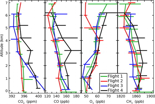
Fig. 2 Species–species scatter plots. Data are coloured according to FLEXPART air mass origin, with calculated modal transport age indicated (in days, between parentheses in the legend, see Section 2.3 for details). Dashed red line represents background CO concentration and observations in hatched area are considered as non-polluted (see Section 3.1). (Left) CO–O₃ scatter plot; (right) same for CO–CO₂.

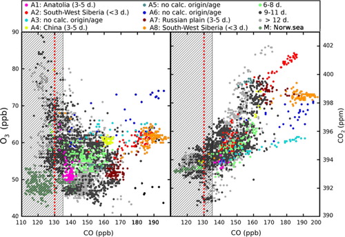
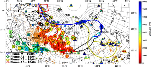
Fig. 3 Back trajectories for four specific plumes including pollution plumes related to biomass burnings and a marine plume, based on ECMWF wind fields. The lines show the mean back trajectory for each one of the four plumes. In addition, every 24 hours each particle cloud's position is divided into four clusters (see text for details), coloured according to their mean altitude. The numbers in each cluster's daily position symbol corresponds to the number of days prior to the particles’ release. The aircraft pathway is highlighted by grey solid line; superposed light blue lines figure plume M observations’ positions. Orange dots are positions of fires detected by the MODIS instrument from 11 to 20 April (from the Fire Information for Resource Management System, available online at http://earthdata.nasa.gov/data/near-real-time-data/firms).

. Campaign description

				Coordinates*
Flight n°	Date UTC	Time UTC	Local time	Latitude	Longitude	Vertical profiles
1	15 Apr. 2010	04:36–10:30	11:36–20:30	55–62°N	83–114°E	10
2	15–16 Apr. 2010	23:04–03:30	09:04–13:30	62–60°N	114–115°E	8
3	16 Apr. 2010	04:47–07:27	14:47–16:27	60–56°N	115–102°E	4
4	18 Apr. 2010	02:20–06:19	11:20–13:19	56–55°N	102–83°E	6

* Coordinates respectively for take-off and landing.

Four flights were carried out from Novosibirsk to Yakutsk and back, with stop-overs in Mirnyy and Bratsk. The campaign took place from 15 to 18 April 2010. Flights were carried out during daytime and under all weather conditions, with the exception of very cloudy conditions. The climate being continental, temperatures in Siberia are still low in April. The mean surface temperatures from 10 to 20 April ranged from 0 to 5°C in southern Siberia to −10°C to the North according to NOAA/ESRL Physical Sciences Division reanalysis (available at http://www.esrl.noaa.gov/psd/data/reanalysis/). The relative humidity was high (>80% near surface during the period of interest). Most of the region where the flights took place was covered by snow.

Both the flight plan and the instrumental package are essentially those described in Paris et al. (2008; see their Fig. 1). A total of 14 ascents/descents were performed by the aircraft during the campaign with a see-saw pattern and with interposed horizontal legs (plateaus) of 10–30 min duration at three different levels: 6600, 2000 and 800 m above ground level. For each of the three levels, 14 horizontal sections were carried out. The Antonov-30 research aircraft used for the campaigns is described by Antokhin et al. (2011) and Paris et al. (2010a).

2.2. Instruments used and data processing

During the flights, concentrations of O₃, CO₂, CO, CH₄ and meteorological (wind speed, temperature, pressure, humidity) data are collected with in situ continuous analysers. The measurement equipment used for the YAK-AEROSIB campaigns is described in Paris et al. (2010a; consult Fig. 3 and Table A1 in the cited reference). Technical details of the instrumentation are summarised in Table 2. The O₃ analyser is based on a commercial instrument (UV absorption; Thermo Instruments Model 49) modified to match aircraft requirements (pressure, temperature, vibrations). The instrument is calibrated in laboratory before and after the campaign with an O₃ generator. The instrument uncertainties are 2 ppb (2%) for an integration time of 4 seconds.

For the 2010 campaign, a CH₄ analyser was added to the instrumental package by the Institute of Atmospheric Optics of Tomsk. Methane was measured here for the first time in the YAK-AEROSIB campaigns, using the Los Gatos Research model FGGA (Fast Greenhouse Gas Analyser). No in-flight calibrations for this instrument were performed but calibration was carried out on the ground both before and after each flight with a standard gas mixture of methane (2308.37±0.802 ppb). Measurements are reported on the Nippon Sanso Company scale maintained by Tohoku University, with an offset of 0.5 ppb relative to the NOAA CH₄ scale (Dlugokencky et al., 2005). Abnormal mixing ratios due to an identified instrument malfunction were filtered out, resulting in a precision of 10–30 ppb depending on flights. Standard deviation (n=90) of the measured standard gas concentration during the pre- and post-flight calibration was 6.18 ppb. The limited precision prevents the detection of narrow plumes in CH₄ data.

Conditions in airborne campaigns (vibrations, thermal and pressure variation) impose recurrent calibrations for CO and CO₂ to compensate for drifts. This prevents the collection of continuous measurements during the entire flight duration. Carbon dioxide calibration gases are traceable to primary World Meteorological Organisation/NOAA standards and drifts are corrected by linear interpolation between the ‘zero’ reference gas injections.

2.3. Air mass origin and back trajectories with the Lagrangian model FLEXPART

The FLEXPART Lagrangian particle dispersion model (Stohl et al., 2005) was used for long-range transport analysis and for determining the origin of the sampled polluted air masses. Two different approaches were implemented. In the first method (‘receptor-oriented’), designed for separating and quantifying remote contributions in a single plume, 20-d retro-plumes were calculated using 60000 computational particles from short segments (0.5×0.5°) along the plume sections of the flight tracks. The model calculations were based on two alternative meteorological data sets to verify consistency of the simulated transport: operational analyses from the National Centres for Environmental Prediction's Global Forecast System (GFS) with a resolution of 0.5°×0.5° and 26 vertical levels and the European Centre for Medium-Range Weather Forecasts’ (ECMWF) model with a resolution of 1°×1° and 91 vertical levels. All the figures were plotted using the ECMWF products. The FLEXPART model output (reported as ns.kg⁻¹) is proportional to the residence time of the particles in a given volume of air and corresponds to potential emission sensitivity (PES). When convolved with the gridded emission fluxes from an emission inventory, maps of potential source contributions (PSC) are obtained. Integrating these maps over the globe yields a model-calculated mixing ratio of the emitted species at the location of the aircraft. EDGAR fast track 2000v3.2 (Emission Database for Global Atmospheric Research from PBL Netherlands Environmental Assessment Agency) was used for anthropogenic CO emissions other than biomass burning. Biomass burning CO emissions were based on fire locations detected with a confidence of more than 75% by the MODIS (Moderate Resolution Imaging Spectroradiometer) instrument onboard the Terra and Aqua satellites (Giglio et al., 2003; data imported from NASA's EOSDIS website; Earth Observing System and Information system; http://earthdata.nasa.gov/data/near-real-time-data/firms) and a land cover classification, as described by Stohl et al. (2007). For every single plume, we estimate the characteristic residence time in the atmosphere using the modal age given as the age of the maximum contribution in the PSC.

The second method (‘flight curtains’) is intended to study the spatial structure of air masses origin in the troposphere nearby the measurement route. Particles were released from a two-dimensional grid oriented as a vertical curtain along the flight track, with 0.5°×0.5°×500 m boxes distributed in the height interval 1000–7000 m. Every release box was filled with 2000 virtual particles for which back trajectories are calculated. Back trajectories have been calculated from the sampling date back to 6 April 2010. For every time step, the fraction of particles originating from pre-selected regions of interest is calculated.

3. Results and discussion

3.1. Average, clean and polluted air masses composition

The overall tropospheric composition measured during the spring 2010 campaign is generally comparable to that observed during previous campaigns (Paris et al., 2008, 2010a 2010b) with a vertical distribution typical of late winter over Siberia. However, the spring 2012 campaign is on average less polluted than the previous spring campaign (2006). The mean CO mixing ratio was 145±22 ppb in 2010, compared to 174±28 ppb in 2006. In spring 2010, air masses came predominantly from clean Arctic regions, whereas in 2006, the main origins were Europe and north-eastern Asia.

Figure 1 shows for each species the median mixing ratio vertical profiles for the four flights. Regarding O₃, the mixing ratios generally increase with altitude (linear regression slope of +1.4±0.03 ppb/km; r=0.87). This small positive O₃ mixing ratio gradient is usually attributed to a stratospheric source and to the surface deposition sink (supposedly limited to snow-free areas; e.g. Engvall-Stjernberg et al., 2012) as well as photochemical production, which is more efficient in the middle and upper troposphere (Reeves et al., 2002). In summer, previous campaigns have shown that the O₃ surface sink is more pronounced resulting in a steeper vertical gradient in the lower troposphere (Paris et al., 2010b). The CO₂ gradient of −0.6 ppm/km (r=−0.90) confirms the limited biogenic activity (confined to plant respiration while vegetation uptake has not started over Siberia in April) that causes the restricted spring O₃ sink. Indeed, the gradient is +1 ppm/km during the summer campaigns, due to a net sink of CO₂ through vegetation uptake (Paris et al., 2010a).

As for CO₂, CO concentrations decrease with altitude (−4.1 ppb/km; r=−0.87), except in Flight 4 when pollution and fire plumes were observed (referred to as Plume A8 below in Section 3.2) in large sections of the flight in mid-troposphere. The same is true for CH₄ (−7.4 ppb/km; r=−0.87). Higher concentrations at lower altitudes are due to the proximity with the surface sources for CO (fossil fuel and biomass burning) and CH₄ (mainly anthropogenic emissions and to a limited extent wetlands in late winter). All these combustion-related emissions are expected to influence indirectly the regional O₃ budget.

Further in the paper, we focus on the influence of remote anthropogenic emissions and biomass burning on O₃ concentrations, from emitting regions to the observed field through transport. Despite the remoteness of most emissions, the observed plumes remained coherent and can be distinguished from the ambient background troposphere. Signatures of combustion-related emissions, traced by CO enhancements, are superimposed on background levels of CO resulting from CH₄ oxidation and the oxidation of biogenic hydrocarbons. Carbon monoxide deviations from this background are used for pollution plume identification. In this analysis of the YAK-AEROSIB campaign, the background is considered as uniform (see also Pommier et al., 2010).

Before going further in plume description, we define, and describe, ‘background’ conditions using the following method. The quartile with the highest CO concentrations (>153 ppb) was considered as polluted and screened out; we also excluded the Plume M (Table 3) described in Section 3.4 which has very different characteristics from the troposphere observed during the rest of the campaign. In the remaining data, any 2-minute interval in the measurement time series with a CO standard deviation above 10 ppb was flagged out. For the remaining intervals, the first quartile of the concentration distribution was used as an estimate for the CO background concentration of the campaign. The CO background concentration is estimated to be 130 ppb during the campaign.

We consider that air masses with ΔCO<5 ppb (relative to the CO instrument uncertainties; see Table 2) can be assimilated to background conditions. During the campaign, the air masses observed in background conditions account for ~33% of the whole data set (Fig. 2, hatched area, excluding plume M in dark green in the figure and described in Section 3.4). In ‘background’ air, CO and CO₂ are correlated (r=0.78, p<0.001). This is explained by the global co-emission of these two species during combustion processes. Carbon monoxide and O₃ in background conditions have opposite vertical concentrations profile slopes, caused by (1) the background O₃ chemistry with low photochemical production or destruction in the low troposphere and transport; (2) the widespread surface CO sources; and (3) the occasional tropospheric propagation of CO-poor, O₃-rich stratospheric air.

Table 2 Instrument characteristics

Species measured	Core technique/instrument	Acquisition frequency	Meas. uncertainties	Calibration frequency	Reference
CO2	NDIR LI-COR 6262	2s	0.15 ppm	30 min or each plateau	Paris et al., 2008
CH4	OA-ICOS LGR FGGA	1s	6 ppb/0.27%	Pre and post flight
CO	Gas filter correlation Thermo 48C	1s*	5 ppb/5%*	20 min	Nédélec et al., 2003
O3	UV absorption Thermo 49	4s	2 ppb/2%		Paris et al., 2008
Aerosols	Diffusional particle sizer	80s	10%	Pre and post flight	Reischl et al., 1991
Relative humidity	HYCAL IH-3602-C Honeywell	1s	7%		Zuev et al., 1992
Temperature		1s	0.5°C		Zuev et al., 1992

* After 30-s slide averaging.

In the following, ΔCO refers to the difference between a CO concentration and the background concentration. We estimate that 40% of the data is ‘polluted’ (defined here as ΔCO>5 ppb). Figure 2 shows scatter plots of CO₂ and O₃ against CO, highlighting polluted air. In polluted air masses, the overall CO–CO₂ correlation is r=0.74 (p<0.001) with a regression slope of 5.5 ppb CO/ppm CO₂. For comparison, the biomass burning emission ratio is about 107 ppb CO/ppm CO₂ (Andreae & Merlet, 2001); the anthropogenic emission ratio is about 9 ppb CO/ppm CO₂ in the EDGARv4.2 inventory for the European Union and reaches 40 ppb CO/ppm CO₂ in the polluted region near Beijing (Wang et al., 2010). Our slope is somewhat smaller than the emission ratio of anthropogenic combustion sources, confirming that mixing with cleaner air during transport and oxidation of CO by OH has taken place.

3.2. Influence of combustion processes on O₃ concentrations

In Fig. 2, plumes are coloured with respect to their origin, along with an estimate of their CO modal age (calculated with FLEXPART as explained in Section 2.3). The CO–O₃ correlations are determined by chemical reactions that can occur during the transport for these two species: CO can be oxidised by OH-radicals; O₃ is produced in the presence of NO_x; O₃ can also be destroyed with NO in the nascent plume, and subsequently produced or destructed in the plume. Negative CO–O₃ correlations are supposedly caused by significant destruction of O₃ during transport. Positive regression slopes significantly higher than for the background conditions can be associated with photochemical O₃ production. When positive correlations are close to the background ones, distinguishing photochemical production, destruction or surface deposition remains challenging. We find no significant CO–O₃ correlations for the whole set of selected observations of polluted air (r ²<0.01), making it difficult to infer any large-scale patterns of production or destruction of O₃ over Siberia during the period of interest. Correlations in individual plumes show high variability between plumes (−0.95<r<0.9). These observations are consistent with the large heterogeneity of possible photochemical patterns in combustion plumes in the free troposphere (for example trans-Atlantic pollution and wildfire plumes observed by Real et al., 2007 and Real et al., 2010). These patterns are strongly dependent on the emission of precursors in the emission region and photochemistry along transport and mixing between air masses.

As we do not have measurements of NO_x and other O₃ precursors, our discussion is based on residence-time with plumes from similar regions having comparable precursor concentrations. We base our discussion of individual plumes on FLEXPART back trajectories and simulated CO enhancements; FLEXPART identified plumes aged of 3–5 d. In Fig. 3, back trajectories for several selected plumes are plotted, superimposed on a map of a MODIS hot spot satellite detection during the period of interest. Every day backwards in time, the released virtual particles are grouped into five clusters, the position of which is indicated by the coloured symbols (the number within them corresponds to the backward time in days); the colour of the symbols are related to their mean altitude. Some plumes originate from south-western Siberia (plumes A2 and A8 in Table 3) and the western Russian plain (plume A7), two populated regions with heavy industry and numerous biomass burning hot spots (mainly agricultural in spring; Korontzi et al., 2006) according to MODIS hot spot satellite detection. In these plumes, we find statistically significant positive CO–O₃ correlations (r>0.60, p<0.001), with regression slopes of 0.1 to 0.8 ppb O₃/ppb CO. Regional anthropogenic activities are likely to emit precursors and hence enhance O₃ mixing ratios downwind in the free troposphere.

Table 3 Selected single plumes and specific events

		Coordinates			Concentrations (mean±1σ dev)				Correlation coef./regression slope
Pl. ID	Time UTC	Lat (°N)	Lon (°E)	Alt (m a.s.l)	CO2 (ppm)	CH4 (ppb)	O3 (ppb)	CO (ppb)	CO/CO2 (ppb/ppm)	O3/CO (ppb/ppb)
A1	15 Apr. 04:45	56.3	84.9	6900	393.8±0.3	1883±13	52.5±3.1	138.6±2.4	−	−0.56 −2.26
A2	15 Apr. 05:20	56.4	85.7	1100	398.0±2.7	1920±12	61±0.0	181.2±6.8	0.97 6.1	0.68 0.33
A3	15 Apr. 23:15	62.6	115.3	4500	394.8±0.6	1838±11	63.2±1.7	171.0±13.7	0.94 27.5	–
A4	16 Apr. 05:15	59.5	112.5	6600	397.4±1.3	1858±19	60.7±0.6	162.3±1.7	–	–
A5	18 Apr. 07:25	56.4	101.8	1000	401.4±0.6	1862±14	54.4±0.6	165.9±4.4	0.74 12.2	–
A6	18 Apr. 04:30	55.7	91.5	5200	396.6±1.1	1860±21	67.5±4.4	174.6±17.5	0.81 12.3	0.56 0.45
A7	18 Apr. 05:15	55.3	88.2	3000	398.4±0.5	1871±17	59.6±1.7	178.5±19.4	0.85 11.0	0.73 0.13
A8	18 Apr. 05:30	55.3	86.3	1600	398.8±0.5	1854±17	52.3±1.7	166.6±2.9	−	0.60 0.81
S	18 Apr. 03:00	55.9	98.5	6700	388.7±0.9	1801±23	177±35.3	90±17	0.57 4.4	−0.92 −2.06
M	16 Apr. 01:00	61.8	121.7	6700	394.1±1.6	1824±22	49±2.2	125±9	0.94 11.1	−0.77 −3.00

Identifiers begin with ‘A’ for anthropogenic (Section 3.2), ‘M’ for ‘marine’ plume (Section 3.4), ‘S’ for stratospheric intrusion (Section 3.3). Coordinates are the average position for the selected plumes. Correlations are indicated only if significant, i.e. p <0.01.

Another young plume (A4 in Table 3 and Fig. 3) with high CO mixing ratios (ΔCO>32 ppb) was calculated to be transported from the Korean peninsula and the eastern Sino-Russian border, where a conveyor belt quickly uplifted the plume. These two regions are industrialised regions with a contribution from biomass burning emissions (about 10% of the FLEXPART calculated CO enhancement is attributed to biomass burning). The plume was observed for about 5 minutes, but calibrations prevented sufficient simultaneous measurements to calculate reliable correlations between species. Nevertheless we observe an overall deficit of O₃ (∣ΔO₃∣>15 ppb) compared to the ambient air observed right before and after the selected plume, where ΔCO=+32 ppb. The O₃ deficit and CO excess can be partly attributed to a non-negligible mixing with air from the planetary boundary layer (PBL), transported by the conveyor belt. Note that more than 15% of the sample resided in the PBL less than 3 d before measurement according to FLEXPART simulations. But if we use the vertical mean gradients calculated in Section 3.1, the O₃ deficit cannot be explained by only PBL influence. We then cannot exclude possible production with subsequent significant destruction in the plume (e.g. Real et al., 2010). An alternative explanation would be O₃ titration within the plume over the source region where there would be high NO_x concentrations. All these plumes well represented by the FLEXPART model are in their first days downwind of the emission, when photochemical regimes cause the steeper O₃ production and/or destruction.

A few polluted plumes are not well simulated by FLEXPART. These plumes with observed high ΔCO and measured in narrow layers are in blue in Fig. 2 (see also positions and average mixing ratios in Table 3; there, plumes A3, A5 and A6). Another plume (A1 in Table 3) with high modal age (>6 d) and ΔCO=10 ppb was not well simulated by FLEXPART. Model limitations including driving wind fields’ resolution, turbulence parameterisations and emission inventories, make the identification of some plumes difficult, especially the oldest ones which tend to be excessively diffused by the model and that we cannot analyse precisely. As a consequence, these inaccuracies in the model prevents a proper analysis of narrow plumes and old ones characterising long-range transport. This deficiency introduces a bias of sampling in our study. Nevertheless, our case studies remain consistent with previous studies with more numerous occurrences of O₃ enhancements than destruction in biomass burning and pollution plume.

3.3. Upper troposphere O₃ excess and stratospheric intrusion

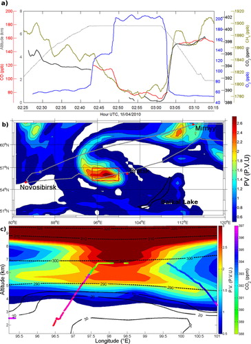
Figure 4a shows an observed decrease in CO and CO₂ mixing ratios and a steep increase in O₃ concentrations during Flight 4 at 7000 m (Plume S in Table 3). In the sampled area (55.9°N, 98.5°E), observed mixing ratios for CH₄, CO and CO₂ were much lower than elsewhere at this altitude (ΔCO₂=−6.0±0.9 ppm; ΔCO=−40.1±17.2 ppb; ΔCH₄=−17±23 ppb compared to the median above 6000 m for the campaign), whereas O₃ (O₃=176.8±35.3 ppb; up to 215 ppb) was three times higher than in the other observations at these altitudes, characteristic of lower stratosphere air. Since the flight was well below the regional mean tropopause altitude during the campaign (300 hPa or ~9000 m in this area on 18 April 2010 according to NOAA/ESRL Physical Sciences Division reanalysis, available at http://www.esrl.noaa.gov/psd/data/reanalysis/), such high O₃ concentrations suggest that stratospheric air must have been mixed into the troposphere earlier, or that a tropopause fold was occurring simultaneously to the flight. The sampling of ‘fresh’ stratospheric air is confirmed by in-situ measured meteorological parameters: the wet bulb potential temperature was 300 K, about 20 K lower than the tropopause mean at this latitude (but almost 5 K higher than measured ambient air at 7000 m in the area), suggesting a quasi-adiabatic intrusion (2000–3000 m descent stretching over about 150 km) of stratospheric air, from the tropopause to mid/upper troposphere.

Over the area where the O₃ excess was measured (spanning roughly 5° by 5°), meteorological datasets (mainly ECMWF potential vorticity fields) suggest a frequency of 20–50 tropopause fold events per year (Beekmann et al., 1997). During frontal episodes, the dry intrusion air stream associated with extra-tropical cyclones generates a positive potential vorticity anomaly associated with the downward flux of stratospheric air. Under these particular circumstances, isentropic transport from stratosphere to troposphere can occur and the tropopause can drop to 320 K (i.e. 300–400 hPa or 6–8 km) for latitudes between 40 and 90°N (Holton et al., 1995).

During Flight 4, the occurrence of a stratospheric intrusion was confirmed by different independent data sets: in situ measured meteorological parameters, satellite imagery and ECMWF analysis fields. The intrusion is associated to a cut-off cyclone (about 150 km wide in its core, with an arm spanning over about 700 km; centred where we observe stratospheric air) with high wind speeds (>30 m.s⁻¹) and high potential vorticity (>2 PVU; potential vorticity units; 1 PVU=10⁻⁶ K.m².kg⁻¹.s⁻¹) high wind speed (about 30 m.s⁻¹), downward flow (about 5 m.s⁻¹, estimated with aircraft mean pitch angle during the intrusion) and high potential vorticity (>2 PVU). A significant downward flux was also estimated using the mean aircraft pitch during the event. We find evidence of this frontal situation in the measured mixing ratios of other trace gases: CO₂ mixing ratios were about 393.5 ppm east of the intrusion, whereas west of the intrusion they were 2.9 ppm higher (396.4 ppm) at the same altitude. These higher CO₂ concentrations coincide with a strong PBL influence as simulated by FLEXPART (Fig. 4c, solid lines). These sharp gradients of O₃ and CO₂ mixing ratio across the intrusion's boundary are linked with the contrasted transport patterns across frontal regions, i.e. the warm conveyor belt lifting PBL air into the middle and upper troposphere, and dry intrusion of stratospheric air. Such sharp chemical composition gradients associated to fronts have been documented, e.g. by Esler et al. (2003) and Vaughan et al. (2003).

Fig. 4 Stratospheric intrusion. (a) Time series for all measured trace gases. CO₂ and CO data are not continuous because of concurrent in-flight calibrations and instrument correction; (b) ECMWF potential vorticity map at 450 hPa (≈5700 m), 18 April 03:00; and (c) Potential vorticity section along aircraft trajectory (coloured regarding CO₂ concentrations). Dashed contours for potential temperature in K and solid contour for PBL origin in % calculated by FLEXPART 1 d before the snapshot.

The FLEXPART backward simulations confirm the stratospheric intrusion, with a long residence time in the stratosphere (more than 7 d in the past 10 d for more than 75% of the sample) prior to detection. FLEXPART associates this stratospheric air mass with long-range transport in the lower stratosphere and upper troposphere. Most of the sampled stratospheric air is calculated to subsequently remain within the troposphere: 90% of the released particles are located in air masses with PV<1.5 PVU and below 6 km after 8 d.

As the observed STE is very well defined both in the observation and in the ECMWF analysis, we use PV/O₃ correlation to estimate the O₃ influx into the troposphere. We take PV from the ECMWF analyses and O₃ from the measurements along the flight track. We find a PV/O₃ correlation with correlation coefficient r=0.90 and a slope of 140 ppb O₃/PVU along the flight track. Assuming that this correlation is typical for the entire dry air stream, we can use PV from ECMWF analyses to estimate the total amount of ozone carried by the dry intrusion. Hence, integrating inside a chosen domain in regards to PV fields (the red square area in Fig. 4b), we obtain an O₃ stratospheric input of 2.56±0.29×10⁷ kg (9.05±0.9×10¹³ kg of air). FLEXPART forward trajectories suggest that 70% of the stratospheric intrusion is well-mixed in the troposphere after 3 d; hence the local flux associated to this event is 70.1±10.5 kg O₃ s⁻¹. The evaluation of the uncertainties in chemistry–transport models (Stohl et al., 1998), especially in STE context (Meloen et al., 2003), is difficult because of, for example, numerical scheme errors, spatial or temporal mismatches and errors in meteorological forcings. The given uncertainties here are upper error limits calculated by convoluting errors at each step of our discussion. Three STE events are visible in Fig. 4b over an area of 2.5×10⁶ km². Assuming that the flux are similar for these events, the corresponding regional flux of O₃ is therefore approximately 9.75±2.9×10¹⁰ molecules O₃ cm⁻² s⁻¹. If we consider that the region and time window that we investigated is large enough to be representative of the spring mean flux over Siberia, our estimation of downward O₃ flux can be compared to climatological studies. This estimation is in the same magnitude of the mean downward flux over Western Europe (12±2.7×10¹⁰ molecules O₃ cm⁻² s⁻¹; Beekmann et al. 1997) and consistent with other studies values (Ancellet et al., 1994). Sprenger and Wernli (2003) carried out a climatological study of STE in the Northern Hemisphere. Their conclusions over Siberia estimated low downward flux in winter (>two times lower than our figure) and downward flux of the same magnitude of our result during summer months. The upper troposphere appears to have been more perturbed than the winter climatology and was closer to its summer state rather during the 2010 late winter campaign.

Atmospheric chemistry transport models tend to poorly represent STE, notably because the filamentary structure of the tropopause folds is lost by numerical diffusion in global circulation models (e.g. Cristofanelli et al., 2003; Roelofs et al., 2003). Detailed in-situ observations of STE, such as the case presented here, are important because they can contribute to model validation at fine spatial and temporal scales.

3.4. Widespread upper tropospheric low O₃ concentrations

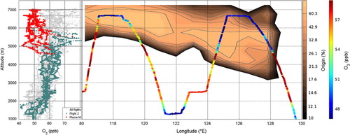
Although O₃ concentrations normally increase with altitude in the troposphere, due to the stratospheric influx and upper troposphere photochemical production, we observed an air mass with low O₃ mixing ratios between 6000 and 7000 m, to the west of Yakutsk, sampled along four level-flight sections at 6700 m (plume M in Table 3 spanning an area of roughly 800×200 km; see Fig. 3). Observed O₃ concentrations in this air mass were 49.2±2.2 ppb, with a ΔO₃=−14 ppb relative to the median for all other flight plateaus above 6000 m. There was a sharp gradient in O₃ concentrations between the surrounding mid-troposphere and the low-ozone air mass (see vertical profile in Fig. 5). CO, CO₂ and CH₄ concentrations were not noticeably different from surrounding air. The concentrations relative to background values were ΔCO=−4.5±9.1 ppb, ΔCO₂ =−0.6±1.6 ppm and ΔCH₄ =+7±22 ppb. As a result, the air mass does not appear to have been influenced by recent emissions from anthropogenic activity or biomass burning with enhanced levels of trace gases.

FLEXPART back trajectories point to similar pathways for all samples within this low-O₃ air mass (Fig. 3). This air mass spent 3 d in the upper troposphere (>5000 m) over the north Siberian coast, then 1–2 d in the middle troposphere (>3000 m) over northern Scandinavia and, finally, 3 d over the Norwegian Sea in the lower troposphere and the PBL. For this period in the backward transport, at least 80% of FLEXPART particles are simulated to have travelled over the Norwegian Sea in the lower troposphere (see red box in Fig. 5). Another plume with similar O₃ mixing ratios (47.3±1.2 ppb) was observed at the same altitude during Flight 1, 15 hours earlier than Flight 2, and has similar back trajectories. Other air masses that have resided over the Arctic Ocean were also observed in the upper troposphere but they did not exhibit low O₃ concentrations (during other flights, O₃>60 ppb in plumes with dominant Arctic origin in the upper troposphere).

Fig. 5 Measured O₃ and air fraction originating from the North Atlantic lower troposphere for Flight 2 (16 April 2010). (Left) O₃ mixing ratios measured during Flight 2 (red and green symbols) are superimposed over the overall campaign data (gray symbols); the air mass originating from North Atlantic at high latitudes is indicated in red; (right) measured O₃ mixing ratios along aircraft pathway over FLEXPART-calculated North Atlantic origin, expressed in % of the original released particle cloud. The North Atlantic area is defined as: 64–71°N, 3°W–10°E, 0–2000 m (see red box in Fig. 3).

A likely explanation would be the transport of an air mass with already low O₃ concentrations over the Norwegian Sea. An air mass with originally low O₃ concentrations and no significant injection of O₃ precursors is likely to remain poor in O₃ during the transport due to reduced O₃ production in the troposphere. It has been observed that the conditions (high H₂O concentrations with low NO_x concentration) in the marine boundary layer tend to cause a net O₃ destruction in the lower troposphere over the North Atlantic (Reeves et al., 2002) and long term measurements in the marine boundary layer point to concentrations of 40 ppb O₃ during spring (Parrish et al., 1998). All the available pieces of information suggest that the observed air mass would have been influenced by marine photochemistry and then transported to East Siberia with a very stable photochemical regime (low O₃ precursor mixing ratios and limited solar radiation in spring in Arctic regions) and almost no mixing with the ambient air rich in O₃ in the upper troposphere. Though less likely, another explanation for the low O₃ concentrations could be the remote influence of the first phase of the Eyjafjallajökull eruption in spring 2010. Forward simulations point to volcanic plumes transported to Siberia with patterns similar to those observed in the upper troposphere. The first phase of the eruption was characterised by no significant emissions of ash and gas compared to the second phase (e.g. Stohl et al., 2011). However, the presence of volcanic fine ashes and/or halogens could possibly have accelerated the O₃ destruction in the observed plumes. This O₃ destruction could have increased the depletion caused by the marine boundary layer influence.

4. Conclusion

A new intensive airborne campaign was carried out in the framework of the YAK-AEROSIB project over Siberia in spring between 15 and 18 April 2010. We analysed backward transport calculated with the Lagrangian model FLEXPART to study processes influencing the O₃ budget in the Siberian troposphere.

The 28 vertical profiles of concentrations of a number of atmospheric species collected during the campaign exhibit slightly increasing CO₂ with decreasing altitude, indicating a net surface source of CO₂ (plant respiration, biomass burning and anthropogenic emissions). A corresponding gradient was also found for CO, suggesting the importance of combustion sources. The O₃ gradient, what is positive with increasing altitude, suggests limited deposition at the surface (especially on leaves and through stomatal activity) and net source in the lower stratosphere and upper troposphere.

We show cases of long-range transport of pollutants and biomass burning plumes that influence O₃ mixing ratios over Siberia by focusing on plumes with CO excess from background conditions as a proxy of combustion processes. Plumes from Russian urban and industrial regions are typically associated with enhanced O₃ concentrations when observed 4–6 d after emission. But low O₃ was also observed in plumes transported from urban region.

An air mass, poor in O₃ (ΔO₃=−20.5 ppb) but with no significant difference in CO and CO₂ concentrations relative to the background, was observed at 6700 m over a large area. The backward transport simulations indicate that the air mass resided for a long time in the lower troposphere over the Norwegian Sea and the Arctic/North Atlantic Ocean 5 d before airborne measurements. This suggests O₃ destruction in the marine boundary layer with no significant recovery due to low O₃ precursor concentrations and little significant mixing with background air masses richer in O₃ than the original marine air mass until the observation.

Our data also indicate a significant contribution of the stratosphere to the tropospheric O₃ budget over Siberia. We have quantified the input of a large stratospheric intrusion over Siberia. A downward flux was observed in a frontal system with huge enhancement in O₃ mixing ratios (+200%, ΔO₃=+150 ppb) and depletion in other trace gases. Observations combined with satellite imagery and ECMWF analysed meteorological fields were precise enough to infer an approximate estimation of transported air in this single STE (2.56±0.29×10⁷ kg O₃). Global estimates and model representation of processes leading to STE would benefit from comparisons with detailed in-situ measurements such as the one described here.

5. Acknowledgements

We thank the scientific and flight crew for their expertise and for carrying out successfully the campaigns since 2006. The measurement campaigns were funded under the project LIA YAK-AEROSIB by the ANR Blanc POLARCAT, CLIMSLIP-LEFE, CNRS, the French Ministry of Foreign Affairs, CEA (in France), and RAS and RFBR (in Russia). A. Stohl was supported by the Norwegian Research Council in the framework of the CLIMSLIP project. Funding support from the French ANR Blanc SIMI 5–6 021 01 Climate Impact of Short-lived Pollutants and Methane in the Arctic (CLIMSLIP) is acknowledged.

References

- Alvarado M. J , Logan J. A , Mao J , Apel E , Riemer D , co-authors . Nitrogen oxides and PAN in plumes from boreal fires during ARCTAS-B and their impact on ozone: an integrated analysis of aircraft and satellite observations. Atmos. Chem. Phys. 2010; 10: 9739–9760.
- Ancellet G , Beekmann M , Papayannis A . Impact of cutoff low development on downward transport of ozone in the troposphere. J. Geophys. Res. 1994; 99: 3451–3468.
- Andreae M. O , Merlet P . Emissions of trace gases and aerosols from biomass burning. Global Biogeochem. Cycles. 2001; 15: 955–966.
- Antokhin P. N , Arshinov M. Yu , Belan B. D , Davydov D. K , Zhidovkin E. V , co-authors . OPTIK-É AN-30 aircraft laboratory for studies of the atmospheric composition. J. Atmos. Ocean. Technol. 2011; 29: 64–75.
- Beekmann M , Ancellet G , Blonsky S , De Muer D , Ebel A , co-authors . Regional and global tropopause fold occurrence and related ozone flux across the tropopause. J. Atmos. Chem. 1997; 28: 29–44.
- Belan B. D , Zadde G. O , Ivlev G. A , Krasnov O. A , Pirogov V. A , co-authors . Complex assessment of the conditions of the air basin over Norilsk industrial region. Part 5. Admixtures in the ground air layer. The correspondence of the air composition to hygienic standards. Recommendations. Opt. Atmos. Okeana. 2007; 20(2): 132–142.
- Browning K. A . The dry intrusion perspective of extra-tropical cyclone development. Meteorol. Appl. 1997; 4: 317–324.
- Cristofanelli P , Bonasoni P , Collins W , Feichter J , Forster C , co-authors . Stratosphere-to-troposphere transport: a model and method evaluation. J. Geophys. Res. 2003; 108: 8525.
- Collins W. J , Derwent R. G , Johnson C. E , Stevenson D. S . The impact of human activities on the photochemical production and destruction of tropospheric ozone. Q.J.R. Meteorol. Soc. 2000; 126: 1925–1951.
- Dlugokencky E. J , Myers R. C , Lang P. M , Masarie K. A , Crotwell , co-authors . Conversion of NOAA atmospheric dry air CH4 mole fractions to a gravimetrically prepared standard scale. J. Geophys. Res. 2005; 110: D18306.
- Elansky N. F . Russian Studies of Atmospheric Ozone in 2007–2011. Izv. Atmos. Ocean. Phys. 2012; 48(3): 281–298.
- Engvall-Stjernberg A.-C , Skorokhod A , Elansky N , Paris J.-D , Nédélec P , co-authors . Low surface ozone in Siberia. Tellus B. 2012; 64: 11607.
- Esler J. G , Haynes P. H , Law K. S , Barjat H , Dewey K , co-authors . Transport and mixing between airmasses in cold frontal regions during dynamics and chemistry of frontal zones (DCFZ). J. Geophys. Res. 2003; 108(D4): 4142.
- Giglio L , Descloitres J , Justice C. O , Kaufman Y . An enhanced contextual fire detection algorithm for MODIS. Rem. Sens. Environ. 2003; 87: 273–282.
- Gilman J. B , Burkhart J. F , Lerner B. M , Williams E. J , Kuster W. C , co-authors . Ozone variability and halogen oxidation within the Arctic and sub-Arctic springtime boundary layer. Atmos. Chem. Phys. 2010; 10: 10223–10236.
- Hauglustaine D. A , Lathiere J , Szopa S , Folberth G. A . Future tropospheric ozone simulated with a climate-chemistry-biosphere model. Geophys. Res. Lett. 2005; 32: L24807.
- Holton J. R , Haynes P. H , McIntyre M. E , Douglass A. R , Rood R. B , co-authors . Stratosphere-troposphere exchange. Rev. Geophys. 1995; 33(4): 403–439.
- Hemispheric Transport of Air Pollution Working Group (HTAP). Dentener F , Keating T , Akimoto H . Hemispheric transport of air pollution: Part A: ozone and particulate matter. Air pollution Studies No. 17. 2010; Geneva: United Nations. 278.
- Ishijima K , Patra P. K , Takigawa M , Machida T , Matsueda H , co-authors . Stratospheric influence on the seasonal cycle of nitrous oxide in the troposphere as deduced from aircraft observations and model simulations. J. Geophys. Res. 2010; 115: D20308.
- Jaffe D. A , Wigder N. L . Ozone production from wildfires: a critical review. Atmos. Environ. 2012; 51: 1–10.
- James P , Stohl A , Forster C , Eckhardt S , Seibert P , co-authors . A 15-year climatology of stratosphere–troposphere exchange with a Lagrangian particle dispersion model: 2. Mean climate and seasonal variability. J. Geophys. Res. 2003; 108: 8522.
- Korontzi S , McCarty J , Loboda T , Kumar S , Justice C . Global distribution of agricultural fires in croplands from 3 years of moderate resolution imaging spectroradiometer (MODIS) data. Global Biogeochem. Cycles. 2006; 20(2): GB2021.
- Meloen J , Siegmund P , van Velthoven P , Kelder H , Sprenger M , co-authors . Stratosphere-troposphere exchange: a model and method intercomparison. J. Geophys. Res. 2003; 108(D12): 8526.
- Nédélec P , Cammas J.-P , Thouret V , Athier G , Cousin J.-M , co-authors . An improved infrared carbon monoxide analyser for routine measurements aboard commercial Airbus aircraft: technical validation and first scientific results of the MOZAIC III programme. Atmos. Chem. Phys. 2003; 3: 1551–1564.
- Oltmans S. J , Lefohn A. S , Harris J. M , Tarasick D. W , Thompson A. M , co-authors . Enhanced ozone over western North America from biomass burning in Eurasia during April 2008 as seen in surface and profile observations. Atmos. Environ. 2010; 44: 4497–4509.
- Paris J.-D , Ciais P , Nédélec P , Ramonet M , Golytsin G , co-authors . The YAK-AEROSIB transcontinental aircraft campaigns: new insights on the transport of CO2, CO and O3 across Siberia. Tellus B. 2008; 60(4): 551–568.
- Paris J.-D , Ciais P , Nédélec P , Stohl A , Belan B. D , co-authors . New insights on the chemical composition of the Siberian air shed from the YAK AEROSIB aircraft campaigns. B. Am. Meteorol. Soc. 2010a; 91(5): 625–641.
- Paris J.-D , Stohl A , Ciais P , Nédélec P , Belan B. D , co-authors . Source-receptor relationships for airborne measurements of CO2, CO and O3 above Siberia: a cluster-based approach. Atmos. Chem. Phys. 2010b; 10: 1671–1687.
- Parrish D. D , Trainer M , Holloway J. S , Yee J. E , Warshawsky M. S , co-authors . Relationships between ozone and carbon monoxide at surface sites in the North Atlantic region. J. Geophys. Res. 1998; 103(D11): 13357–13376.
- Pommier M , Clerbaux C , Law K. S , Ancellet G , Bernath P , co-authors . Analysis of IASI tropospheric O3 data over the Arctic during POLARCAT campaigns in 2008. Atmos. Chem. Phys. 2012; 12: 7371–7389.
- Pommier M , Law K. S , Clerbaux C , Turquety S , Hurtmans D , co-authors . IASI carbon monoxide validation over the Arctic during POLARCAT spring and summer campaigns. Atmos. Chem. Phys. 2010; 10: 10655–10678.
- Real E , Law K. S , Weinzierl B , Fiebig M , Petzold A , co-authors . Processes influencing ozone levels in Alaskan forest fire plumes during long-range transport over the North Atlantic. J. Geophys. Res. 2007; 112(D10): D10S41.
- Real E , Pisso I , Law K. S , Legras B , Bousserez N , co-authors . Toward a novel high-resolution modeling approach for the study of chemical evolution of pollutant plumes during long-range transport. J. Geophys. Res. 2010; 115: D12302.
- Reeves C. E , Penkett S. A , Bauguitte S , Law K. S , Evans M. J , co-authors . Potential for photochemical ozone formation in the troposphere over the North Atlantic as derived from aircraft observations during ACSOE. J. Geophys. Res. 2002; 107(D23): 4707.
- Reischl G. P , Majerowicz A , Ankilow A , Eremenko S , Mavliev R . Comparison of the Novosibirsk automated diffusion battery with the Vienna electromobility spectrometer. J. Aerosol Sci. 1991; 22: 223–228.
- Roelofs G. J , Kentarchos A. S , Trickl T , Stohl A , Collins W. J , co-authors . Intercomparison of tropospheric ozone models: Ozone transport in a complex tropopause folding event. J. Geophys. Res. 2003; 108(D12): 8529.
- Seinfeld J. H , Pandis S. N . Atmospheric chemistry and physics: From air pollution to climate change. 2006; Hoboken, NJ: John Wiley. 2nd ed.
- Shakina N. P , Ivanova A. R , Elansky N. F , Markova T. A . Transcontinental observations of surface ozone concentration in the TROICA experiments: 2. The effect of the stratosphere-troposphere exchange. Izv. Atmos. Ocean. Phys. 2001; 37(Suppl. 1): S39–S48.
- Sommar J , Andersson M. E , Jacobi H.-W . Circumpolar measurements of speciated mercury, ozone and carbon monoxide in the boundary layer of the Arctic Ocean. Atmos. Chem. Phys. 2010; 10: 5031–5045.
- Sprenger M , Wernli H . A northern hemispheric climatology of cross-tropopause exchange for the ERA15 time period (1979–1993). J. Geophys. Res. 2003; 108(D12): 8521.
- Stohl A . A one-year Lagrangian “climatology” of airstreams in the northern hemisphere troposphere and lowermost stratosphere. J. Geophys. Res. 2001; 106(D7): 7263–7279.
- Stohl A , Berg T , Burkhart J. F , Forster C , Herber A , co-authors . Arctic smoke: record high air pollution levels in the European Arctic due to agricultural fires in Eastern Europe in spring. Atmos. Chem. Phys. 2007; 7: 511–534.
- Stohl A , Forster C , Frank A , Seibert P , Wotawa G . Technical note: the Lagrangian particle dispersion model FLEXPART version 6.2. Atmos. Chem. Phys. 2005; 5: 2461–2474.
- Stohl A , Hittenberger M , Wotawa G . Validation of the Lagrangian particle dispersion model FLEXPART against large scale tracer experiment data. Atmos. Environ. 1998; 24: 4245–4264.
- Stohl A , Prata A. J , Eckhardt S , Clarisse L , Durant A , co-authors . Determination of time- and height-resolved volcanic ash emissions and their use for quantitative ash dispersion modeling: the 2010 Eyjafjallajökull eruption. Atmos. Chem. Phys. 2011; 11: 4333–4351.
- Stohl A , Wernli H , James P , Bourqui M , Forster C , co-authors . A new perspective of stratosphere-troposphere exchange. Bull. Am. Meteorol. Soc. 2003; 84(11): 1565–1574.
- Thomas J. L , Raut J.-C , Law K. S , Marelle L , Ancellet G , co-authors . Pollution transport from North America to Greenland during summer 2008. Atmos. Chem. Phys. 2013; 13: 3825–3848.
- Vaughan G , Garland W. E , Dewey K. J , Gerbig C . Aircraft measurements of a warm conveyor belt—a case study. J. Atmos. Chem. 2003; 46: 117–129.
- Verma S , Worden J , Pierce B , Jones D. B. A , Al-Saadi J , co-authors . Ozone production in boreal fire smoke plumes using observations from the tropospheric emission spectrometer and the ozone monitoring instrument. J. Geophys. Res. 2009; 114: D02303.
- Wang Y , Munger J. W , Xu S , McElroy M. B , Hao J , co-authors . CO2 and its correlation with CO at a rural site near Beijing: implications for combustion efficiency in China. Atmos. Chem. Phys. 2010; 10: 8881–8897.
- Wernli H , Sprenger M . Identification and ERA-15 climatology of potential vorticity streamers and cutoffs near the extratropical tropopause. J. Atmos. Sci. 2007; 64: 1569–1586.
- Wild O , Pochanart P , Akimoto H . Trans-Eurasian transport of ozone and its precursors. J. Geophys. Res. 2004; 109: D11302.
- Zuev V. E , Belan B. D , Kabanov D. M , Kovalevskii V. K , Luk'ianov O. I , co-authors . The Optik-E AN-30 laboratory-airplane for ecological studies. Opt. Atmos. Okeana. 1992; 5: 1012–1021.