Modelling of growing season methane fluxes in a high-Arctic wet tundra ecosystem 1997–2010 using in situ and high-resolution satellite data

Abstract

Methane (CH₄) fluxes 1997–2010 were studied by combining remotely sensed normalised difference water index (NDWI) with in situ CH₄ fluxes from Rylekærene, a high-Arctic wet tundra ecosystem in the Zackenberg valley, north-eastern Greenland. In situ CH₄ fluxes were measured using the closed-chamber technique. Regression models between in situ CH₄ fluxes and environmental variables [soil temperature (T_soil), water table depth (WtD) and active layer (AL) thickness] were established for different temporal and spatial scales. The relationship between in situ WtD and remotely sensed NDWI was also studied. The regression models were combined and evaluated against in situ CH₄ fluxes. The models including NDWI as the input data performed on average slightly better [root mean square error (RMSE) =1.56] than the models without NDWI (RMSE=1.67), and they were better in reproducing CH₄ flux variability. The CH₄ flux model that performed the best included exponential relationships against temporal variation in T _soil and AL, an exponential relationship against spatial variation in WtD and a linear relationship between WtD and remotely sensed NDWI (RMSE=1.50). There were no trends in modelled CH₄ flux budgets between 1997 and 2010. Hence, during this period there were no trends in the soil temperature at 10 cm depth and NDWI.

• NDWI
• methane
• Arctic
• Landsat
• climate change

1. Introduction

High-latitude ecosystems are identified to be vulnerable to climate change and there is substantial evidence for effects of climate warming in the Arctic (Christensen et al., 2004; Johansson et al., 2006; Tarnocai, 2006) leading to permafrost degradation, melting of snow, glaciers and sea ice, lengthening of the growing season, a shift in plant species composition, increased emissions of methane (CH₄) and carbon dioxide (CO₂) and increased plant productivity (Oechel et al., 1993; Svensson et al., 1999; Serreze et al., 2000; Christensen et al., 2004; Malmer et al., 2005; Johansson et al., 2006; Tarnocai, 2006). In the centuries to come, Arctic areas are projected to experience more pronounced changes in temperature, precipitation and length of the growing season than the rest of the world (ACIA, 2005; IPCC, 2007). These climatic variables have strong effects on the land–atmosphere exchange of CH₄ and CO₂, indicating risks of positive feedback mechanisms (e.g. Christensen et al., 2004; Johansson et al., 2006). Northern wet tundra ecosystems play a key role in controlling the terrestrial carbon cycle, and approximately 50% of the global soil organic carbon is today stored in the northern permafrost regions (Smith et al., 2004; McGuire et al., 2009; Tarnocai et al., 2009). Wet tundra ecosystems are also ideal sites for CH₄ production, and the atmospheric input of CH₄ from northern latitude wetlands accounts for about 25% of the total natural CH₄ sources globally (Schlesinger, 1997). Excluding the effect of water vapour, CH₄ has contributed to approximately 22% of the greenhouse effect during the past 150 yr (IPCC, 2007). The land–atmosphere exchange of CH₄ is the sum of the methanogenesis in the wet anaerobic part of the soil and the methanotrophy in the aerated upper part of the soil. The net CH₄ flux is highly dependent on water table depth (WtD), soil temperature, ecosystem productivity, species composition, and for permafrost environments date of snowmelt and active layer (AL) thickness (see Appendix A.1 for abbreviations and symbols; Bubier and Moore, 1994; Friborg et al., 2000; Mastepanov, 2010). As a consequence of climate change, changes in vegetation composition and site-specific variations in emissions of CH₄ and CO₂ have already been reported from sub-Arctic and Arctic areas (Oechel et al., 1993; Svensson et al., 1999; Christensen et al., 2004; Malmer et al., 2005; Johansson et al., 2006; Thompson et al., 2006).

The CH₄ fluxes in Arctic ecosystems are not only varying in the temporal domain but there is also a strong spatial component. For example, several studies have shown a correlation between the spatial variation in WtD and the CH₄ fluxes (Hargreaves and Fowler, 1998; Huttunen et al., 2003; Wille et al., 2008). For accurate assessments of landscape-level CH₄ fluxes, it is necessary to estimate its spatial variation. Assessing landscape-level emissions using manual field-based measurements is time consuming, and remote sensing tools can be used. Optical remote sensing uses measures of surface reflectance to model and map ground characteristics on landscape to global scales. Reflectance within the short-wave infrared (SWIR) wavelengths is known to be highly sensitive to water content of the ground and atmosphere (Lillesand et al., 2008). Variation in reflectance in the SWIR bands is also affected by the internal leaf structure, leaf dry matter content, soil mineral composition and organic matter content (Whiting et al., 2004; de Alwis et al., 2007). Consequently, the SWIR bands alone are not appropriate for estimating hydrological conditions. The near-infrared (NIR) bands are affected by the same ground properties as the SWIR bands, except that the absorption by vegetation liquid water is negligible. Gao (1996) hereby proposed a vegetation index, the normalised difference water index (NDWI), using NIR and SWIR bands to estimate vegetation liquid water. The NDWI has also been applied for estimates of water stress on gross primary production, plant phenology, land cover classification and soil water saturation (Boles et al., 2004; Xiao et al., 2004; Delbart et al., 2005; de Alwis et al., 2007).

The primary aim of this study is to investigate the applicability of combining in situ and high-resolution satellite data for modelling growing season CH₄ fluxes. The drivers of CH₄ fluxes at different temporal and spatial scales were investigated by relating in situ CH₄ fluxes to environmental variables using regression models. The resultant models were used to scale-up the in situ CH₄ fluxes to landscape and inter-annual scales. For the up-scaling, the relationship between in situ soil hydrology and remotely sensed measures of ecosystem moisture content (NDWI) was also studied. The final aim is to investigate trends in growing season CH₄ fluxes, 1997–2010, in a high-Arctic wet tundra ecosystem in north-eastern Greenland.

2. Materials and methods

2.1. Site description

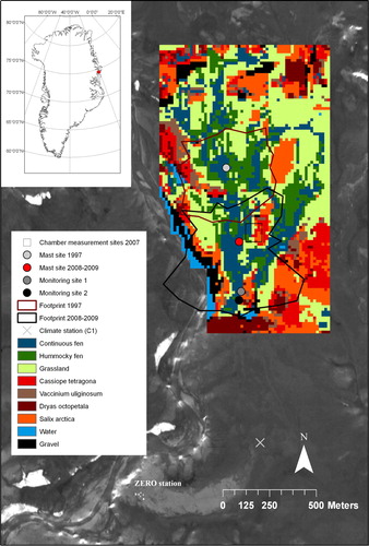
The study was done in Rylekærene (dunlin fens) in the Zackenberg valley (74°28′N 20°34′W), located in the Northeast Greenland National Park. Rylekærene is a patterned wet tundra ecosystem characterised by alternating sequences with high, dry heath areas and low, wet fen areas. These sequences are mainly orientated in strings perpendicular to the hydrologic flow, which goes from NE to SW. The Zackenberg valley is subject to a relatively mild climate for the high-Arctic zone with an average temperature of 5.8°C in the warmest month of the year (July) and mean annual temperature of −9°C (Hansen et al., 2008). The Zackenberg valley is underlain by continuous permafrost and the AL thickness ranges from 0.5 to 1.0 m. The dominant plant communities in the Zackenberg valley are continuous fen (flat areas dominated by Eriophorum scheuchzeri, Carex stans and Dupontia psilosantha), and hummocky fen (hummocks dominated by Eriophorum triste, Salix arctica and Arctagrostis latifolia), grassland (dominated by A. latifolia, E. triste and Alopecurus alpinus), S. arctica snowbed, Cassiope tetragona heath, Dryas octopetala heath and Vaccinium uliginosum heath (Fig. 1); which are distributed spatially due to topography, hydrology and soil type (Elberling et al., 2008). The moss species at the site was dominated by Tomenthypnum, Scorpidium, Aulacomnium and Drepanoclaudus. Since 1995, extensive ecological, biogeographic, climatic and hydrological research and monitoring have been carried out in the Zackenberg research area (Meltofte and Rasch, 2008). The Rylekærene area in this study is the 1.4 km² area covered by the vegetation composition map in Fig. 1.

Fig. 1 The Zackenberg valley and the investigation area surrounding the research station (ZERO). The field inventory map of the dominant plant communities estimated in the Rylekærene study site is superimposed over the area. The vegetation map is the studied area referred to as Rylekærene throughout the text. The red dot on the Greenland map is the location of Zackenberg. The Footprint areas are the average 80% cumulative flux distances of the two towers.

2.2. In situ measurements

2.2.1. Chamber measurements of CH₄ fluxes.

In 2007, a site in the centre of the Rylekærene was chosen so as to encompass the main plant communities dominating the fen within a reasonably small area (~600 m²) (Fig. 1). A total of 55 plots were randomly distributed within the different plant communities; five plots each in the C. tetragona heath, Dryas octopetala heath, V. uliginosum heath and Salix arctica snowbed, 10 plots each in hummocky fen and grassland and 15 plots in continuous fen. CH₄ fluxes were measured in each of the plots using the closed-chamber technique (Livingston and Hutchinson, 1995). A laser off-axis integrated cavity output spectroscopy analyser (LGR, DLT200 Fast Methane Analyzer, Los Gatos Research, USA) was used to measure chamber concentration of CH₄. Measurements were performed 11 times on the 55 plots between 30 June and 4 August 2007. To avoid bias due to measurements at different times of the day in different plant communities, measurements were distributed over the day, such that every second measurement in an individual plots was performed during the morning after 10 a.m., and every second time during the afternoon no later than 6 p.m.

The chamber was a transparent Plexiglas cube of 0.3 m height and a ground area of 0.34 m². The outlet and inlet for gases were located on one of the chamber sides, 0.15 and 0.25 m above the ground, respectively. Two small fans were located in the upper part of the chamber to ensure proper mixing of the chamber headspace and representative sampling. The chamber was vented to minimise artefacts due to changes in pressure or temperature (Livingston and Hutchinson, 1995). Care was taken to avoid induction of an efflux of CH₄ as the chamber was placed on the soil. Collars inserted in the ground were not used during the measurements, but to ensure a proper seal between the chamber and the soil, the chamber was placed in ~2 cm notches inserting the chamber into the ground. The notches were constructed in the start of the growing season, before the measurements started.

Methane concentrations in the chamber were measured every second over the course of 3 min. Concentrations were first measured under daylight conditions, then in the dark, by covering the chamber with a lightproof hood. The chamber was ventilated for 1.5 min between the measurements. Ordinary least-square linear functions were fitted to the concentration change in the chamber over the measurement cycle. The slope of the line was used to calculate the CH₄ fluxes according to Livingston and Hutchinson (1995). Fifteen percent of the chamber measurements were removed due to problems in chamber installation, causing initial ebullition (peak in CH₄ concentration after the chamber installation) or leakage (noisy time series without linear trends in CH₄ concentration).

2.2.2. Environmental variables.

Soil temperature at 10 cm depth (T ₁₀), WtD (centimetres below moss surface) (for the fen communities) and AL (centimetres below moss surface) was measured simultaneously with the chamber-based CH₄ flux measurements between 30 June and 4 August 2007. Water table depth was measured in small holes in close proximity to the chamber measurement plots, and AL was measured with a metal rod driven in to the ground until it reached the top of the permafrost. Soil temperature at 10 cm depth was measured with a 125 mm digital temperature probe (Viking, Eskilstuna, Sweden). The 10 cm depth was chosen as a good proxy of the temperature of the depth of maximum potential CH₄ production at the site which is between 5 and 15 cm (Joabsson and Christensen, 2001).

Soil temperature at 10 cm depth has been continuously measured at the climate station (C1) between 1996–2004 and 2006–2010 (Jensen and Rasch, 2011), from July 2007 to October 2010 at monitoring site 1 (Mastepanov, 2010) and in July–August 2000 at monitoring site 2 (Fig. 1; Joabsson and Christensen, 2001). Water table depth was measured in small holes in the centre of Rylekærene at 26, 1 and 5 sites during the growing seasons of 2008, 2009 and 2010, respectively. In addition, WtD was measured at monitoring sites 2 and 1 during the growing seasons of 2000 and 2007–2010, respectively (Joabsson and Christensen, 2001; Mastepanov, 2010). In 1997, Friborg et al. (2000) measured WtD at the 1997 tower site (Fig. 1). AL thickness was measured at monitoring site 1 in 2007, 2008 and 2009, and at monitoring site 2 in 2000 (Joabsson and Christensen, 2001; Mastepanov, 2010). In 1997, Friborg et al. (2000) measured AL at the 1997 tower site (Fig. 1).

Following Tamstorf et al. (2007), the growing season was assumed to extend from the day of year (DOY) for snow melt to the first of two consecutive days with a soil temperature at 2.5 cm of 0°C or below. Soil temperature data at 2.5 cm depth were taken from C1 (Jensen and Rasch, 2011). Snow depths have been monitored 1998–2010 at C1 (Jensen and Rasch, 2011). The bottom of the Zackenberg valley is relatively flat, and the conditions at C1 are hereby also representative of the studied Rylekærene area. The DOY when snow depths decreased below 10 cm at C1 was used as a proxy for DOY of snowmelt. For 1997, modelled snow cover in the Zackenberg valley from Buus-Hinkler et al. (2006) was used to estimate DOY of snowmelt (Tagesson et al., 2012a).

2.3. Remote sensing data

Data from the moderate resolution imaging spectroradiometer (MODIS) were used in a pre-analysis for determining the average peak season of the NDWI during 2000–2010. Single grid cell subsets (grid size: 500 m×500 m) of the growing season 8-d surface reflectance composites were extracted from the MODIS/Terra L3 collection (MOD09A1) from March 2000 to October 2010 (ORNL DAAC, 2010). The grid cell chosen was from the centre of the Rylekærene. The reflectance data were filtered based on MODIS QC criteria. The NDWI was calculated using surface reflectance data from MODIS according to the following:1

where ρ _NIR is the reflectance in the NIR band, and ρ _SWIR is the reflectance in the SWIR band. Average values and standard deviations (SDs) for the period 2000–2010 were calculated for each 8 d period from the start until the end of the growing season. Based on the MODIS growing season NDWI, the period between 38 and 55 d after DOY of snowmelt was chosen to represent the NDWI peak season (Fig. 2). The MODIS-based NDWI was never used in the actual modelling of CH₄ fluxes. Data of higher spatial resolution were required for the actual analysis, Landsat TM and ETM+ images (grid size: 30 m×30 m) obtained at the NDWI peak seasons of 1997–2010 were chosen for the analysis (Table 1). The NDWI could be affected by precipitation; hence, images with precipitation within 3 d before the DOY of the satellite images were rejected. Images of the chosen satellite are given in Table 1.

Fig. 2 Average (±1 SD) normalised NDWI based on MODIS surface reflectance data 2000–2010. Data was averaged for each 8-d period after DOY of snowmelt and it was normalised against the seasonal average NDWI. The dotted lines show the time window used for choosing high-resolution Landsat data day 38–55 after DOY of snowmelt.

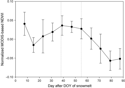
Table 1 The different sensors recording the Landsat images that were used in the analysis

Year	Satellite sensor	DOY of Landsat image	DOY with 10 cm snow depth
1997	Landsat 5 TM	222	170^a
2000	Landsat 7 ETM+	204	165
2002	Landsat 7 ETM+	214	171
2007	Landsat 7 ETM+^c	210	159
2008	Landsat 7 ETM+^c	222	175
2009	Landsat 7 ETM+^c	199	152^b
2010	Landsat 7 ETM+^c	219	167

Day of year (DOY) when the images were obtained is also included. The DOY of 10 cm snow depth for the different years, which was used as start of the growing season, is also given.

^aDOY of 10 cm snow depth based on snow coverage by Buus-Hinkler et al. (2006).

^bIn 2009, the snow depth was by far the shallowest on record and peaked at 17 cm. It was therefore below 10 cm already DOY 136 according to snow depth measurements at C1. In the central parts of the fen, it was visually seen to melt DOY 152.

^cImages taken when the Scan Line Corrector on Landsat 7 was broken.

To compare images between dates and years, all Landsat imagery was converted into reflectance and atmospheric and terrain corrections were performed with ATCOR 3 (version 6.2; Richer, 2005). This method uses look-up tables derived using the Modtran^® 4 radiative transfer code covering a wide range of weather conditions, sun angles and ground elevations. Finally, NDWI based on the Landsat data in Table 1 was calculated according to eq. (1).

2.4. Data analysis

2.4.1. Correspondence between soil hydrology and NDWI.

The WtD measured at the DOY of the satellite images in Table 1 was extracted from the WtD time series for each plot and year. The extracted WtD data were averaged for each satellite pixel. Water table depth measurements within two satellite pixels were removed from the analysis, as these pixels covered the edge of the fen and hereby had large fractions of both heath and fen areas. The WtD were measured only in the fen area (a few metres into the fen) and were not representative of the combined heath/fen-covered satellite pixel. The NDWI do not measure the actual soil hydrology, but rather the effect of soil hydrology on the ground vegetation. The soil hydrology were therefore categorised into seven categories based on our WtD data (WtD_cat); >0 cm (category 0), 0 to >−1.0 cm (category 1), −1 to >−2.0 cm (category 2), −2.0 to >−3.5 (category 3), −3.5 to >−5.0 cm (category 4), −5.0 to>−8.0 (category 5) and<−8.0 cm (category 6). The NDWI was averaged for each WtD_cat. A linear regression between WtD_cat and average NDWI was fitted as follows:2

where u is the intercept and w is the slope of the linear regression (for results, see Section 3.1.2). A reduced major-axis linear regression was chosen as errors were assumed in both variables. The normality assumptions for residuals were checked throughout the study using the Kolmogorov–Smirnov test. The statistics was regarded as significant at a p-value threshold of 0.05.

2.4.2. Correspondence between CH₄ fluxes and environmental variables.

We performed repeated-measures ANOVA, with a Tukey's post hoc test assuming equal variances among groups to test if the in situ CH₄ fluxes differed between the plant communities and between CH₄ flux for light and dark conditions.

The chamber-based CH₄ fluxes were averaged for each of the 11 measurement occasions for both continuous and hummocky fen. The T ₁₀ and WtD measured at monitoring station 1 were averaged for the same 11 occasions. To determine which of the measured environmental variables that best described the temporal variation in CH₄ fluxes and to find model parameters for the subsequent CH₄ flux modelling, simple and multiple ordinary least-square linear and exponential regression functions were fitted between the averaged CH₄ fluxes and the averaged T ₁₀, WtD and AL.

In addition, the spatial relationship between environmental variables and CH₄ fluxes was investigated. The CH₄ fluxes and T ₁₀ measured over the growing season were averaged for each measurement plot. The relationship between spatial variation of CH₄ fluxes and WtD and T ₁₀ was analysed separately for continuous and hummocky fen by fitting linear and exponential least-square regression functions between plot-averaged CH₄ fluxes on average T ₁₀ measured in the vicinity of each plot, and WtD measured at the day of the satellite image 2007 (DOY 210, 29 July).

2.5. The CH₄ flux models

2.5.1. Models estimating temporal variation of CH₄ flux.

Based on the outcome of the correlations previously described under Section 2.4.2 (for results see Section 3.1.1), four regression models were constructed from the fitted functions for further analysis. The models differed in the functional form and in choice of predictor variables included (T ₁₀, WtD, AL or a combination of these). Workflow of the model development and evaluation is visualised in Fig. 3. The models were parameterised for continuous and hummocky fen using non-linear least-square regression analysis in the software SPSS Statistics Version 19. Model 1 represents CH₄ flux () as an exponential function of T ₁₀ as follows:3

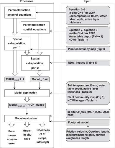
Fig. 3 Workflow for the model development and the model evaluation. The white boxes are steps in the work process of the model development or the model evaluation. The grey boxes are input data or equations going into the models. The thick arrows indicate steps in the work process, whereas thin arrows indicate input. The final results of the model evaluation were the root mean square error, the model-in situ ratio and the goodness-of-fit given by a linear regression equation.

where a is the intercept of the curve and c is the growth constant.

Model 2 was based on eq. (3), with the addition of a term to represent the effect of AL, as parameterised by Friborg et al. (2000) as follows:4

where AL_max is the peak AL measured during the growing season.

Model 3 expresses the CH₄ flux as a linear function of WtD and an exponential function of T ₁₀ as follows:5

where a, b and c are fitted parameters.

Model 4 adds the effect of AL, following Friborg et al. (2000), to eq. (5) as follows:6

Models 1–4 estimate the temporal variation in CH₄ flux over the growing seasons.

2.5.2. The spatial extrapolation of the modelled CH₄ fluxes.

To estimate the CH₄ flux for the entire Rylekærene area, models 1–4 were spatially extrapolated on all pixels with continuous and hummocky fen areas in the vegetation map (Fig. 1). The remaining pixels containing grassland, heath, gravel and water were given a modelled CH₄ flux value of zero since no CH₄ fluxes were detected from these areas at any time during the growing season (for results see Section 3.1.1). The subscript ‘nosat’ is used hereinafter to refer to these models, as they do not include satellite data as input data.

In addition, the modelled CH₄ fluxes from Model_nosat 1–4 were spatially extrapolated over the studied Rylekærene area based on remotely sensed NDWI. To estimate the contribution in CH₄ flux of an individual plot in comparison to the average CH₄ flux from all plots (hereafter referred to as , the plot-averaged CH₄ fluxes () were divided by the average CH₄ flux for all plots (), treating the continuous and hummocky fen data sets separately as follows:7

This gave a fraction of how the CH₄ fluxes vary spatially in relationship to the average. The measured WtD at DOY 210 (29 July) 2007 at each chamber measurement point was assigned to a WtD_cat category, as described in Section 2.4.1. An exponential regression of against plot WtD_cat was thereafter fitted, for both continuous and hummocky fen as follows:8

where k is the intercept of the exponential curve and l is the growth constant. This provided a relationship to estimate the relative CH₄ flux at any point against the average, as a function of the WtD_cat at that point.

The previously derived WtD_cat–NDWI relationship [eq. (2), Section 2.4.1] gives satellite-based WtD_cat images. Applying eq. (8) to these WtD_cat images create images. The images can subsequently be multiplied with the CH₄ fluxes modelled with the Model_nosat 1–4, and the CH₄ fluxes for each satellite pixel in the entire Rylekærene are hereby estimated as follows:9

where k and l are the constants from eq. (8), and u and w are constants from eq. (2). The first term of eq. (9) on the right-hand side, represents the spatial variation in relationship to the average of the area, whereas the second term on the right-hand side [eqs. (3–6)] of eq. (9), represents the temporal variation in CH₄ flux. These models are named Model_sat 1–4 hereinafter, and the subscript ‘sat’ is used as these models include satellite-based NDWI.

2.6. Evaluation of the models

2.6.1. In situ CH₄ flux data used for model evaluation.

For the evaluation of the regression models, a number of different data sets were used. During the growing seasons 2008 and 2009, fen-scale CH₄ fluxes were measured by combining the eddy covariance technique with atmospheric gradients and the K-theory (Tagesson et al., 2012b). We also used data from Friborg et al. (2000), who similarly measured fen-scale CH₄ fluxes during the growing season of 1997, with the eddy covariance technique. The footprints of the towers were estimated with a footprint model developed by Hsieh et al. (2000) based on the Obukhov lengths, given by sonic anemometer data, the measurement heights and the surface roughness length. The measurement height of the EC system was 2.7 m in 1997. For 2008 and 2009, measurement heights in the footprint model were set to the arithmetic (1.73 m) and the geometric (1.39 m) mean of the measurement heights of the concentration gradient, for stable and unstable conditions, respectively (Horst, 1999). Momentum roughness length was set to 0.01 m (Wieringa, 1993; Mölder and Kellner, 2002). The flux footprint model gives a footprint-weighed function estimating the relative contribution of the different parts of the tower footprint. The average 80% cumulative flux distances of the two towers are shown in Fig. 1. Finally, we used closed-chamber measurements of CH₄ fluxes from the study of Joabsson and Christensen (2001) covering six continuous fen plots at monitoring site 2 during the growing season of 2000 (Fig. 1).

2.6.2. Evaluation of temporally and spatially extrapolated CH₄ fluxes.

Model_nosat 1–4 and Model_sat 1–4 were evaluated against the in situ CH₄ fluxes for 1997, 2000 and 2008–2009. The T ₁₀, WtD and AL observations for 1997, 2000 and 2008–2009 (Table 2) were used as the model input data. Monitoring sites 1 and 2 are 45 m apart, and situated along the same edge of the fen. It was therefore assumed that the environmental variables were similar between the two sites. In 1997, WtD was not measured at either of the monitoring sites 1 and 2, and Model_nosat 3–4 and Model_sat 3–4 were thus not applied for this year.

Table 2 Monitored environmental variables used in the modelling of CH₄ fluxes

Year	T 10	WtD	AL
1997	M1^a	–	T1997
2000	M2^b	M2	M2
2002	M1^a	–	M1^c
2007	M1^d	M1	M1
2008	M1	M1	M1
2009	M1	M1	M1
2010	M1	–	M1

T ₁₀ is the soil temperature at 10 cm depth, WtD is the water table depth and AL is the active layer thickness. Gaps in the data series were filled by linear interpolation. The ‘–’ either means that no measurements were done, or that they were not necessary in the modelling process. M1 is the monitoring site 1, M2 is the monitoring site 2 and T1997 is the Tower site 1997 (Fig. 1).

^a T ₁₀ modelled with a linear regression fitted between T ₁₀ at monitoring site 1 d 1–57 of the growing seasons 2007, 2008 and 2009 and T ₁₀ at C1 (R ²=0.47, n=4147).

^b T ₁₀ was measured from the 8 July 2000. At the start of the growing season, a linear regression fitted between hourly averaged T ₁₀ at monitoring site 2 in 2000 and hourly T ₁₀ at C1 (R ²=0.89, n=1062) was used.

^cAL modelled with a linear regression fitted between AL at monitoring site 1 of the growing seasons 2007, 2008 and 2009 and AL at ZEROCALM1 (Jensen and Rasch, 2011) (R ²=0.96, n=23).

^d T ₁₀ was measured from the 4 July 2007. At the start of the growing season, a linear regression fitted between hourly values of T ₁₀ at monitoring site 1 and C1 (R ²=0.80, n=1531) for the growing season 2007, was used.

Model_nosat 1–4 were applied on all pixels with continuous and hummocky fen areas in the vegetation map (Fig. 1) separately for 1997, 2000 and 2008–2009. The remaining pixels containing grassland, heath, gravel and water were given a modelled CH₄ flux value of zero.

For Model_sat 1–4, the CH₄ fluxes from Model_nosat 1–4 were used for the second term of eq. (9). For the first term of eq. (9), NDWI estimates of the satellite images from 1997, 2000, 2008 and 2009 in Table 1 were used as input data. Combined, eq. (9) gave the CH₄ fluxes for each satellite pixel in the entire Rylekærene.

The relative contribution of the different parts of the tower footprint was estimated with a footprint-weighed function (Hsieh et al., 2000) (see Section 2.6.1). This relative contribution of the different parts of the tower footprint was taken times the Model_nosat 1–4 and Model_sat 1–4 maps to estimate the modelled CH₄ fluxes for the same areas as measured with the towers.

The CH₄ fluxes were modelled for each half-hour that was measured with the micrometeorological measurements 1997 and 2008–2009. For evaluation against the chamber measurements, the CH₄ fluxes were modelled for the same point in time as the chamber measurements were conducted. Daily averages were calculated with modelled and in situ CH₄ fluxes. Finally, the daily-averaged Model_nosat 1–4 and the daily-averaged Model_sat 1–4 from the footprint area of the towers were evaluated against the daily-averaged tower-based CH₄ fluxes 1997 and 2008–2009 (Friborg et al., 2000; Tagesson et al., 2012b). It was also evaluated against the chamber-based CH₄ flux measurements from 2000 at monitoring site 2 (Joabsson and Christensen, 2001). The model-in situ data agreements were quantified as the root mean square error (RMSE), the model-in situ ratio, and by goodness-of-fit when a least-square linear regression was fitted between average modelled CH₄ fluxes against the averaged in situ fluxes.

2.7. Growing season CH₄ fluxes 1997–2010

Equation (4) parameterised for continuous and hummocky fen was used in eq. (9) to model CH₄ fluxes 1997–2010. The T ₁₀ and AL data in Table 2 and the NDWI images in Table 1 were used as input data to eq. (9).

Average modelled CH₄ fluxes day 1–57 of the growing season were calculated for the entire Rylekærene area. Only day 1–57 were used due to the results of the model evaluation (see Section 3.2). Accumulated CH₄ fluxes day 1–57 of the growing seasons were calculated to estimate a CH₄ flux budgets for Rylekærene for the different years. The uncertainties of the models for the different years were estimated by calculating model standard errors (SEs) using the formula for error propagation (see Appendix A.2). In addition, average T ₁₀ measured at C1 day 1–57 of the growing season was calculated 1996–2004 and 2007–2010. Maximum MODIS-based NDWI from the peak period of the growing season was extracted for 2000–2010.

3. Results

3.1. The relationships to environmental variables

3.1.1. CH₄ flux and environmental variables.

In the 2007 chamber flux measurements, no CH₄ fluxes were statistically different from zero for the grassland, S. arctica snowbed, C. tetragona heath, Dryas octopetala heath or V. uliginosum heath plots (Table 3). However, on 11% of the heath and S. arctica snowbed measurements we observed negative CH₄ fluxes (Table 3). There were significant differences between the CH₄ fluxes in continuous and hummocky fen (p<0.0001). They were therefore treated as two categories in the subsequent data analysis. There were, however, no significant differences between CH₄ fluxes measured in dark and light conditions for either continuous (p=0.965) or hummocky fen (p=0.998). We therefore chose to combine light and dark measurements in the subsequent data analysis. Average CH₄ fluxes measured between 10 a.m. and 6 p.m. during the period 30 June –4 August 2007 were 9.1±5.3 (± 1 SD) mg CH₄ m⁻² h⁻¹, and 3.6±2.5 mg CH₄ m⁻² h⁻¹, for continuous and hummocky fen, respectively.

Table 3 Average (±1 SD) CH₄ fluxes and environmental variables measured between 10 a.m. and 6 p.m. in the period 30 June–4 August 2007, for the different plant communities

Plant communities	T 10 (°C)	WtD (cm)	ALmax (cm)	CH4 flux (mg CH4 m^−2 h^−1)	Sample size
Continuous fen	7.4±1.3	−3.4±3.6	49±3	9.1±5.3	154
Hummocky fen	7.4±1.3	−8.2±4.2	47±4	3.6±2.5	108
Grassland	6.0±1.3	–	56±8	0.1±0.4	110
Salix snowbed	8.2±2.1	–	78±3	−0.04±0.04	51
Vaccinium Heath	7.6±2.3	–	69±5	−0.02±0.04	54
Cassiope heath	7.7±1.6	–	74±6	−0.03±0.03	54
Dryas heath	8.9±2.1	–	75±5	−0.03±0.03	54

The T ₁₀ is the average soil temperature at 10 cm depth and WtD is the average water table depth (centimetres below moss surface) measured 21 June–4 August 2007. AL_max is the average active layer thickness (centimetres below moss surface) from the 4 August 2007, when the thickest AL was measured.

Water tables from 30 June –4 August 2007 were on average 3.4 and 8.2 cm below the ground surface for continuous and hummocky fen, respectively. No free-standing water was detected in the ALs of Grassland, S. arctica snowbed, C. tetragona, Dryas octopetala and V. uliginosum heath. The thickest average AL measured on 4 August, ranged from 47 to 78 cm, for the different plant communities (Table 3). Plant communities at elevated and drier locations had a thicker AL than the plant communities in the wetter locations.

There were close relationships between temporal variation in CH₄ fluxes and T ₁₀ for continuous and hummocky fen. The function with the best correlation was exponential for hummocky fen (Table 4 and Fig. 4a). For continuous fen, the linear and exponential functions were equally well correlated (Table 4 and Fig. 4a). The exponential function was chosen for further analysis, as it is theoretically more correct (e.g. Dunfield et al., 1993). There were also linear correlations with WtD for both continuous and hummocky fen (Table 3 and Fig. 4b). The AL measurements started at ~24 cm depth, and we did hereby not measure CH₄ fluxes at any shallow AL. The AL increased throughout the growing season whereas CH₄ flux decreased in the end of the season, and this resulted in a negative linear correlation between CH₄ flux and AL (data not shown). In the subsequent modelling analysis including effects of AL, we therefore apply the parameterisation by Friborg et al. (2000).

Fig. 4 The relationship between temporal variation in CH₄ fluxes to (a) averaged soil temperature at 10 cm depth and (b) averaged water table depth. Equation (3) is given in the text.

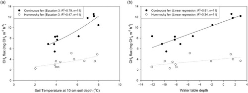
Table 4 Parameters for the models relating temporal variation in CH₄ fluxes and temporal variation in environmental variables

Plant communities	Equation	Environmental variables	a	b	c	d	R ^2
Continuous fen	Linear	WtD	11.11±0.47	0.41±0.07	–	–	0.81
Hummocky fen	Linear	WtD	4.10±0.35	0.10±0.05	–	–	0.34
Continuous fen	Eq. (3)	T 10	4.50±0.63	–	0.13±0.02	–	0.79
Hummocky fen	Eq. (3)	T 10	2.14±0.45	–	0.10±0.04	–	0.47
Continuous fen	Eq. (4)	T 10, AL	4.41±0.59	–	0.13±0.02	0.17±0.15	0.76
Hummocky fen	Eq. (4)	T 10, AL	1.97±0.36	–	0.11±0.03	0.17±0.15	0.54
Continuous fen	Eq. (5)	WtD, T 10	7.38±2.54	0.17±0.15	0.06±0.05	–	0.85
Hummocky fen	Eq. (5)	WtD, T 10	2.31±0.98	0.01±0.06	0.10±0.05	–	0.47
Continuous fen	Eq. (6)	WtD, T 10, AL	7.38±2.54	0.17±0.15	0.06±0.05	0.17±0.15	0.85
Hummocky fen	Eq. (6)	WtD, T 10, AL	2.31±0.98	0.01±0.06	0.10±0.05	0.17±0.15	0.47

Linear means a linear regression. Equations (3)–(6) are given in the text. a, b and c are fitted parameters, d was parameterised by Friborg et al. (2000), and R ² is the coefficient of determination.

3.1.2. The spatial relationships to environmental variables.

There was no correlation between spatial variation in CH₄ fluxes and T ₁₀, but significant exponential relationships between spatial variation in CH₄ fluxes and WtD at the DOY of the satellite image 2007 were found (Fig. 5).

Fig. 5 Plot-averaged CH₄ fluxes against spatial variation in water table depth at the DOY of the satellite image 2007 (DOY 210).

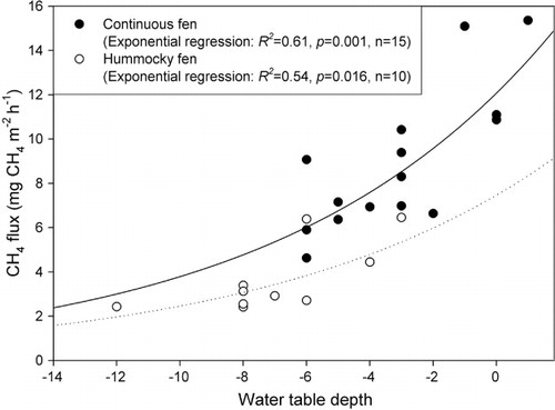
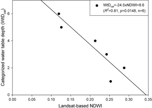
Exponential regression of on plot WtD_cat [eq. (8)] gave an R ² of 0.61 for continuous fen (, n=15) and 0.49 for hummocky fen (, n=10). There was a significant relationship between in situ measurements of WtD_cat and remotely sensed NDWI (Fig. 6).

Fig. 6 Categorised water table depth (WtD_cat) against Landsat-based NDWI averaged for each WtD_cat category. None of the satellite pixels had an average water table above the soil surface, and there is hereby no zero WtD_cat.

3.2. Model evaluation

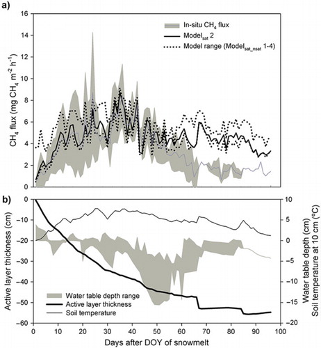
The first 57 d after snowmelt, the in situ CH₄ fluxes were generally well described by the models; modelled CH₄ fluxes averaged for all models were 1.07 of in situ CH₄ flux (Fig. 7a). Some models overestimated the CH₄ flux in the start of the growing season, and approximately 57 d after DOY of snowmelt variables not included in any of the models seemed to constrain in situ CH₄ fluxes for all years and average modelled CH₄ fluxes were on average 2.48 times the in situ CH₄ fluxes (Fig. 7a). The models reproduce the pattern of the in situ fluxes well also in the end of the growing season, but they overestimated the fluxes considerably. In the further model evaluation, only modelled CH₄ fluxes from days 1–57 after DOY of snowmelt will be used. The temporal variation in the input data is shown in Fig. 7b.

Fig. 7 (a) In situ and modelled CH₄ flux and (b) input variables against day after day of year (DOY) of snowmelt. The in situ CH₄ flux is the average±1 SD averaged for each day after DOY of snowmelt 1997, 2000, 2007 and 2008. The modelled CH₄ flux is the average flux modelled by Model_sat 2 for each day after DOY of snowmelt 1997, 2000, 2007 and 2008. Model_sat 2 was chosen as it was the best model according the model evaluation. The model range is the minimum and the maximum of the eight models averaged for each day after DOY of snowmelt 1997, 2000, 2007 and 2008. The water table depth range is the minimum and maximum of the measured values for each day after DOY of snowmelt 1997, 2000, 2007 and 2008. Active layer thickness and soil temperature at 10 cm depth is the average for each day after DOY of snowmelt 1997, 2000, 2007 and 2008.

As can be seen in Table 5, there is on average not a large difference in model performance between the eight models. Model_sat 1–4 showed a slightly better correspondence (lower RMSE) to in situ CH₄ flux in comparison to the respective Model_nosat 1–4 (Table 5). In addition, CH₄ fluxes from Model_sat 1–4 were on average closer to the in situ values [average ratio from 1997, 2000, 2008 and 2009: 1.07±0.14 (±1 SD)] than Model_nosat 1–4 (ratio: 1.18±0.35) (Table 5). However, and most importantly, from the SDs (Model_sat: 0.14 vs. Model_nosat: 0.35) it can be seen that there were large differences in how well the models reproduced the inter-annual variations in the in situ CH₄ fluxes. The smaller SDs for Model_sat indicate that they reproduced inter-annual variation better than Model_nosat. The linear function fitted between average modelled and average measured values was also better correlated, the fitted curve was closer to a one-to-one relationship, and the intercept was closer to zero (Fig. 8a). This indicates that the models including NDWI as an explanatory variable were better in reproducing CH₄ flux variability.

Fig. 8 Modelled CH₄ fluxes against in situ CH₄ fluxes. (a) Average of modelled CH₄ fluxes for all Model_nosat and Model_sat to show the difference between models with and without satellite-based NDWI; (b) Model_sat 2 and Model_sat 4 against in situ CH₄ fluxes to illustrate the difference between models including and excluding the temporal variation in WtD; (c) Model_sat 1 and Model_sat 2 against in situ CH₄ fluxes to illustrate the difference between models including or excluding the effect of AL; and (d) Modelled CH₄ fluxes modelled with Model_sat 2 for the different years against in situ CH₄ fluxes.

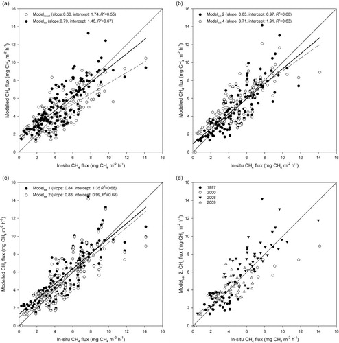
Table 5 Ratios of modelled CH₄ fluxes to in situ CH₄ fluxes for the different years and the different models

Model	Equation	1997	2000	2008	2009	Mean all years	RMSE
1nosat	(3)	0.88	1.59	0.83	1.32	1.16±0.36	1.64
2nosat	(4)	0.83	1.48	0.78	1.17	1.07±0.33	1.58
3nosat	(5)		1.63	0.85	1.43	1.31±0.40	2.10
4nosat	(6)		1.52	0.80	1.25	1.19±0.36	1.84
Mean allnosat		0.86	1.55	0.82	1.30	1.18±0.36	1.67
1sat	(9_3)	1.09	0.87	1.20	1.15	1.08±0.15	1.61
2sat	(9_4)	1.03	0.78	1.13	1.03	0.99±0.15	1.50
3sat	(9_5)		0.96	1.24	1.25	1.15±0.16	1.94
4sat	(9_6)		0.87	1.15	1.09	1.04±0.15	1.62
Mean allsat		1.06	0.87	1.18	1.13	1.07±0.14	1.56

Root mean square errors (RMSE) in mg CH₄ m⁻² h⁻¹ for the different models are also included.

Model_sat 3 including temporal variations in WtD showed a weaker correspondence with measured data (larger RMSE) overall than the other models (Table 5). Model_sat 4, which also included temporal variations in WtD, showed similar correspondence as Model_sat 1. In addition, when temporal variations in WtD were not included the fitted linear functions were better correlated, the regression lines were closer to a one-to-one relationship, and the intercept were closer to zero (Fig. 8b). Including growing season variation in WtD in the models thus decreased the model performance.

Finally, the linear regression analysis showed that Model_sat 1 and Model_sat 2 were equally well correlated to in situ CH₄ fluxes. The fitted curves were equally close to a one-to-one relationship whereas the intercept was slightly closer to zero for Model_sat 2 (Fig. 8c). However, the model with the best correspondence (lowest RMSE) to the in situ CH₄ fluxes was Model_sat 2 (Table 5). Including AL in the models did, therefore, increase the model performance. The model evaluation indicated that all eight models performed well, but the model that performed the best was Model_sat 2 (Table 5 and Fig. 8d).

3.3. Modelled CH₄ fluxes 1997–2010

Modelled CH₄ flux budgets accumulated for the first 57 d of the growing season ranged between 1.8 and 4.1 g CH₄ m⁻² for Rylekærene over the period 1997–2010 (Fig. 9). Although there were large inter-annual variations in CH₄ fluxes, no clear trend was observed (Fig. 10). The modelled CH₄ fluxes over the study period was on average 2.0 mg CH₄ m⁻² h⁻¹ with a model SE of 1.7 mg CH₄ m⁻² h⁻¹ (Table 6), indicating a wide model uncertainty. A clear correlation was apparent between the CH₄ fluxes and MODIS-based peak growing season NDWI (R ²=0.80, n=6). There was also a correlation between the CH₄ fluxes and T ₁₀ at climate station C1 for days 1–57 of the growing season (R ²=0.48, n=7). No significant changes in growing season T ₁₀, or NDWI were apparent over the study period Fig. 10).

Fig. 9 CH₄ fluxes modelled by Model_sat 2, averaged for the Rylekærene area, and accumulated over the first 57 d of the growing seasons 1997–2010.

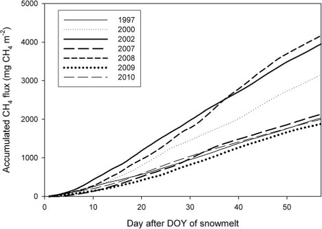
Fig. 10 (a) Accumulated modelled CH₄ fluxes day 1–57 of the growing season for Rylekærene; (b) maximum MODIS-based NDWI for the NDWI peak period of the growing seasons in Rylekærene 1997–2010; and (c) and average soil temperature at 10 cm soil depth at C1 day 1–57 of the growing season. The gap in the soil temperature 2005 was caused by broken soil temperature sensors.

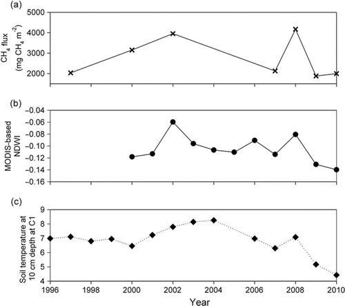
Table 6 Average (± 1 model SE) modelled CH₄ fluxes for the entire Rylekærene area for the first 57 d of the growing season

Year	CH4 fluxes (mg CH4 m^−2 h^−1)
1997	1.5±1.2
2000	2.3±1.1
2002	2.9±3.7
2007	1.6±1.0
2008	3.0±5.3
2009	1.4±0.8
2010	1.5±0.6

The model used for these estimates was the Model_sat2. The variation in CH₄ fluxes due to heterogeneity in the modelled area is not included in the model SEs and it is strictly an estimate of the model uncertainty.

4. Discussion

4.1. Environmental controls on growing season CH₄ fluxes

In wetlands, CH₄ is produced by methanogens under anaerobic conditions and oxidised by methanotrophs in the aerobic parts of the soil. The primary factor determining the distribution of anaerobic and aerobic conditions in wetlands is the combined influence of water and organic matter. Oxygen diffuses about 10⁴ times more slowly through water than through air, and organic matter supports a large biotic oxygen demand that consumes oxygen faster than it is replaced by diffusion (Megonigal et al., 2007). Consequently, it is not surprising that we found CH₄ emissions from continuous and hummocky fen that both had shallow water tables, whereas they were undetectable in the dry plant communities (grassland, S. arctica snowbed and the heath communities) without a free-standing water table. Furthermore, the continuous fen had a water table close to the soil surface (Table 3 and Fig. 5), and consequently the largest CH₄ fluxes. Continuous fen also had a high coverage of vascular plants. Vascular plants both act as conduits, facilitating the CH₄ transport from the anaerobic parts of the soil to the atmosphere, bypassing the aerobic oxidation zone (Bubier and Moore, 1994) and affect the substrate availability for methanogens (Ström et al., 2012).

The darkening of the chamber did not have any direct effects on the in situ CH₄ fluxes during our short chamber enclosure of 3 min, and this indicates that the CH₄ fluxes were not directly affected by stomatal closure. An explanation could be a weak or slow response of stomatal closure to a sudden switch to dark conditions, as has been shown for other wetland plants (Torn and Chapin, 1993). An alternative explanation is that most of the CH₄ fluxes were occurring through other pathways than through the stomata (Morrissey et al., 1993).

As expected, soil temperature influenced the temporal variability in CH₄ fluxes strongly; the metabolic activity of both methanogens and methanotrophs is related exponentially to temperature (e.g. Dunfield et al., 1993). The response of CH₄ fluxes to soil temperature was equally well explained by a linear function for continuous fen. The different temperature dependencies for continuous and hummocky fen might be explained by spatially varying factors, such as substrate availability, hydrological conditions, metabolic activity of the methanotrophs or resistances along the transport pathways of CH₄ from the site of production to the atmosphere (Bubier and Moore, 1994). It could be that these spatially varying factors also explain the lack of spatial relationship between CH₄ flux and soil temperature. Another explanation could be the low spatial variation in soil temperature across the measurement area.

A strong correlation between both temporal and spatial variations in CH₄ fluxes and WtD was observed in 2007 (Fig. 4b and 5). In 2007, the measurements started late in the growing season, and as the WtD decreased over the growing season, so did the CH₄ fluxes. Water table depth affects the CH₄ fluxes, delimiting the zones for CH₄ production and oxidation. Still, the model evaluation indicated that including temporal variation in WtD decreased the performance of the CH₄ flux models (Fig. 8b) (for further discussion, see Section 4.3).

An additional factor influencing the zone for CH₄ production is the active layer thickness. The major part of the CH₄ production originates from the root zone where there are readily available substrates for decomposition (Joabsson and Christensen, 2001). AL depth hereby exerts a stronger effect at the start of the growing season when AL is shallow, than later, when it is thicker. In 2007, the measurements started late in the growing season, and CH₄ fluxes were already approaching their peak. An increase in AL did hereby not affect the CH₄ fluxes and this can possibly explain the negative relationship between AL and CH₄ flux seen in the 2007 data.

4.2. The relationship between soil hydrology and NDWI

There was a strong relationship between WtD_cat and NDWI (Fig. 6), indicating a relationship between moisture content of the ground vegetation and the hydrological content in the soil. It should be noted that NDWI is a vegetation index sensitive to changes in plant liquid content at the leaf and canopy level (e.g. Gao, 1996). Normalised difference water index does not sense the absolute WtD, and it is hereby important not to interpret changes in the index as solely related to soil hydrology as it is strictly measuring ground surface properties. In a homogenous ground surface, such as the fen area in Rylekærene, the soil hydrology directly influences the growth patterns of the surface vegetation (Cronk and Fennessy, 2001). Wu et al. (2013) showed that plant biomass, vegetation cover and plant height were strongly correlated to wetland soil moisture. Previously, de Alwis et al. (2007) used NDWI to monitor temporal and spatial variations in surface water content and Goswami et al. (2011) showed that the normalised difference surface water index (NDSWI) was strongly correlated to surface hydrology for an Arctic wetland in Alaska. A similar water index to NDWI, the shortwave infrared water stress index (SIWSI), was shown to be strongly correlated to soil moisture in Senegal (Fensholt and Sandholt, 2003). In addition, in Fig. 2 it can be seen that the NDWI is not strictly following the plant phenology; high values were observed for the start of the growing season when high WtD (Fig. 7b) could be an additional factor affecting the index.

4.3. Validity of the modelled CH₄ fluxes

While the models performed well on average for the first 57 d, i.e. ~69%, of the growing season (Table 5), they should be used with care. The temporal variation in modelled CH₄ flux was strongly related to the soil temperature (Fig. 4a and Fig. 7). This relationship has been shown to be site-dependent, as previous studies have shown both strong relationships (Hargreaves et al., 2001; Rinne et al., 2007; Wille et al., 2008) and relationships that were weak or absent (Wickland et al., 2006; Sachs et al., 2008), as also observed for the continuous and hummocky fen in our study. The dependency of CH₄ flux to soil temperature should therefore be investigated carefully before applying these models to other areas.

At the end of the growing season, the T ₁₀ was still high, resulting in relatively high CH₄ fluxes according to the models (Fig. 7a and 7b). However, the field-measured CH₄ fluxes were decreasing strongly at the end of the growing season. An explanation could be that the vegetation senescence results in lower substrate availability (Ström et al., 2012) and lower vascular plant-mediated CH₄ transport. The vegetation senescence can be seen in the sharp decrease in NDWI after day 57 after DOY of snowmelt (Fig. 2).

Dynamics of the AL is an important factor for subsurface processes and including the effect of AL increased the accuracy of the modelled CH₄ fluxes. The AL is constantly decreasing over the growing season (Fig. 7b), and this increases the zone for CH₄ production. The increase follows the temporal variation in the CH₄ flux for the start of the growing season. At the end of the growing season, when AL is thick, CH₄ fluxes were instead restricted, and a change in AL presumably no longer had a major effect on the fluxes.

The models that included WtD as explanatory variable generally overestimated CH₄ flux in the start of the growing season (high values in model range in Fig. 7a). In addition, the regression analysis indicated that including temporal variation in WtD decreased the model performance (Fig. 8b). The WtD was at its peak at the start of the growing season, closely following snow melt, decreasing over the summer as runoff and evapotranspiration reduced soil water content (Fig. 7b). At the start of the growing season, CH₄ fluxes were uniformly low; most likely, low soil temperatures, low AL and undeveloped vegetation limited CH₄ flux more than WtD. At the end of the growing season, WtD was again increasing, possibly due to temporal patterns in precipitation and evapotranspiration (Hasholt et al., 2008).

Water table depth still affects the CH₄ flux and the models performed better when remotely sensed NDWI was included, thereby accounting both for the inter-annual and spatial variation in ecosystem moisture content. Previous studies showing a positive relationship between CH₄ fluxes and WtD have also mainly showed spatial and long-term dependencies (Huttunen et al., 2003; Bubier et al., 2005; Pelletier et al., 2007; Rinne et al., 2007; Sachs et al., 2008; Wille et al., 2008). An additional explanation for why models incorporating NDWI performed better than the other models is that NDWI not only provides a metric of the ecosystem moisture content; it is also a proxy for vegetation density. This has two positive effects for the modelling of CH₄ flux. First, aerenchymatous species thrive in wet areas, and high NDWI values should hereby indicate a high density of vascular plants. Second, higher vegetation index values also indicate higher primary productivity (e.g. Tagesson et al., 2012a), representing enhanced substrate availability for methanogens (Joabsson and Christensen, 2001).

Previous studies have reported climate-related changes in vegetation composition in sub-Arctic and Arctic areas (Oechel et al., 1993; Malmer et al., 2005). The models derived in this study, however, implicitly assume constant plant community composition in Rylekærene over the period 1997–2010. Changes in plant communities, especially between plants with and without aerenchyma could bias the modelling of CH₄ emission (Oechel et al., 1993; Malmer et al., 2005). However, due to a lack of data on the vegetation dynamics of Rylekærene over the study period, no conclusions as to the possible influence of community composition on CH₄ variability can be drawn.

5. Conclusions

This study has addressed the spatial and temporal extrapolations of in situ measured data, a critical need within research on CH₄ fluxes from the Arctic. Our main aim is to investigate the applicability of combining in situ measurements with a remotely sensed vegetation index, NDWI, for spatial extrapolation of in situ-based CH₄ fluxes. Exponential and linear relationships between CH₄ fluxes and soil temperature, WtD and AL were used to estimate temporal variation in CH₄ fluxes. A spatial relationship between CH₄ flux and WtD was combined with a relationship between WtD and NDWI to spatially extrapolate the CH₄ fluxes. The evaluation of the models indicated that it was applicable to combine in situ measurements of CH₄ flux and NDWI for modelling growing season fluxes. On average, all models performed well, but the models including satellite-based NDWI reproduced the CH₄ flux variability better than the models not including NDWI. Even though the models performed well at this specific site, we would like to emphasise that further investigations are necessary before applying this model approach to other areas. Normalised difference water index, used here primarily as a proxy for WtD, is a vegetation index and attention should be paid to other site-specific factors, such as heterogeneous vegetation composition and soil type, that affect the index. All models overestimated the fluxes at the end of the growing season. A possible explanation could be that the vegetation senescence results in lower substrate availability and lower vascular plant-mediated CH₄ transport. Including these factors as predictors could be a way to improve the models in the future.

We found that the temporal variation in modelled CH₄ flux is strongly related to the soil temperature, WtD and AL thickness. However, we could also see that there are strong site differences in the dependency of CH₄ flux to soil temperature, and this relationship should therefore be investigated carefully before being applied to other areas. Incorporating a relationship between temporal variability in CH₄ flux and WtD decreased the model performance. Water table depth was high in the start and the end of the growing season when CH₄ flux was more constrained by other variables. However, spatial variability in CH₄ flux was strongly related to WtD and including NDWI (ecosystem moisture content) increased the model performance. This indicates that WtD mainly has spatial and long-term effects.

The model that performed best included soil temperature, AL and NDWI as explanatory variables. It was used for investigating trends in the CH₄ fluxes 1997–2010 at the studied high-Arctic wet tundra ecosystem. There was large inter-annual variation in modelled CH₄ fluxes; however, no distinct trend in CH₄ fluxes was seen over the study period. This may suggest that this area had fairly stable CH₄ fluxes over the study period, or that the main factors affecting the CH₄ fluxes have not changed significantly over this period. Indeed, no consistent trends were apparent in soil temperature at 10 cm depth and satellite-based NDWI.

6. Acknowledgement

This study was carried out as part of Lund University Center for Studies of Carbon Cycle and Climate Interactions (LUCCI). The work was funded by the Swedish Research Council FORMAS. We are also grateful to the National Environmental Research Institute, Aarhus University, Denmark and personnel at Zackenberg field station for logistic support.

7. Appendix

A.1. Abbreviations and symbols (Table A )

Table A Abbreviations, symbols and their descriptions

Abbreviation or symbol	Description
a, b, c and d	Model parameters in Equations (3)–(6)
AL	Active layer thickness
ALmax	Peak active layer thickness measured during the growing season
C1	Climate station (Fig. 1)
DOY	Day of year
	Methane flux
	Average chamber-measured methane fluxes from all plots
	Plot-averaged chamber measured methane fluxes
	Fraction of CH4 flux of an individual plot in relation to the average CH4 flux from all plots
k	Intercept of exponential regression between and WtDcat [eq. (8)]
l	Growth constant of exponential regression between and WtDcat [eq. (8)]
M1	Monitoring site 1
M2	Monitoring site 2
Modelnosat	Model data that do not include remote sensing data
Modelsat	Model data that do include remote sensing data
MODIS	Moderate resolution imaging spectroradiometer
NDWI	Normalized difference water index
NIR	Near-infrared wavelengths (780–900 nm)
RMSE	Root mean square errors
	Model standard deviation
	Standard deviation of a model parameter
	Standard deviation of a model parameter
SWIR	Short-wave infrared wavelengths (1000–3000 nm)
SD	Standard deviation
SE	Standard error
T 10	Soil temperature at 10 cm depth
T1997	Tower site 1997
u	Intercept of linear regression between WtDcat and NDWI [eq. (2)]
w	Slope of linear regression between WtDcat and NDWI [eq. (2)]
WtD	Water table depth
WtDcat	Categorized water table depth
y	Year

A.2. Calculation of model standard errors

As the model contained several modelled variables, the formula for error propagation was used to estimate the model SD () (Leo, 1994).A.2.1

where and is SD of model parameters. To simplify, we only give an equation for two variables here. However, in the SD calculations, we included errors from the five parameters in Model 2 [a, c and d in eq. (4); k, l, in eq. (9)], errors in the WtD_cat modelled from NDWI, and finally for some of the years, errors from the parameters in the modelling of soil temperatures and AL. Finally, model SEs were calculated by dividing the SD with square root of the sample size. The variation in CH₄ fluxes due to heterogeneity in the modelled area was not included in the model SE since average values of the modelled area were first calculated. It is strictly an estimate of the model uncertainty.

The average and SD of all model parameters was calculated in the fitting of the regressions. As the WtD was categorised after the linear regression between WtD_cat and NDWI, the SDs of the model parameters could not be used in the calculation of the model SDs. The SD of the WtD_cat was estimated by a Monte–Carlo sampling approach, for both continuous and hummocky fen. The slope (w) and intercept (u) between categorised WtD and NDWI was sampled randomly in a normal distribution around the average 2000 times. These 2000 sets of parameters were included into eq. (2), which were applied to each NDWI image in Table 1 for Rylekærene 1997–2010. Each of the 2000 estimates was classified into its respective WtD_cat. Average and SDs of the 2000 WtD_cat estimates for Rylekærene were then calculated, for both continuous and hummocky fen.

References

- ACIA. Arctic Climate Impact Assessment. 2005; New York: Cambridge University Press.
- Boles S. H , Xiao X , Liu J , Zhang Q , Munkhtuya S , co-authors . Land cover characterization of temperate East Asia using multi-temporal VEGETATION sensor data. Remote. Sens. Environ. 2004; 90: 477–489.
- Bubier J. L , Moore T. R . An ecological perspective on methane emissions from northern wetlands. Trends. Ecol. Evol. 1994; 9: 460–464.
- Bubier J , Moore T , Savage K , Crill P . A comparison of methane flux in a boreal landscape between a dry and a wet year. Glob. Biogeochem. Cycles. 2005; 19: GB1023.
- Buus-Hinkler J , Hansen B. U , Tamstorf M. P , Pedersen S. B . Snow-vegetation relations in a high Arctic ecosystem: inter-annual variability inferred from new monitoring and modeling concepts. Remote. Sens. Environ. 2006; 105: 237–247.
- Christensen T. R , Johansson T , Åkerman H. J , Mastepanov M , Malmer N , co-authors . Thawing sub-arctic permafrost: effects on vegetation and methane emissions. Geophys. Res. Lett. 2004; 31: L04501.
- Cronk J. K , Fennessy M. S . Wetland Plants: Biology and Ecology. 2001; CRC Press, Boca Raton, FL.
- de Alwis D. A , Easton Z. M , Dahlke H. E , Philpot W. D , Steenhuis T. S . Unsupervised classification of saturated areas using a time series of remotely sensed images. Hydrol. Earth. Syst. Sci. 2007; 11: 1609–1620.
- Delbart N , Kergoat L , Le Toan T , Lhermitte J , Picard G . Determination of phenological dates in boreal regions using normalized difference water index. Remote. Sens. Environ. 2005; 97: 26–38.
- Dunfield P , knowles R , Dumont R , Moore T. R . Methane production and consumption in temperate and subarctic peat soils: response to temperature and pH. Soil. Biol. Biochem. 1993; 25: 321–326.
- Elberling B , Tamstorf M. P , Michelsen A , Arndal M. F , Sigsgaard C , co-authors . Meltofte H , Christensen T. R , Elberling B , Forchhammer M. C , Rasch M . Soil and plant community-characteristics and dynamics at Zackenberg. Advances in Ecological Research- High Arctic Ecosystem Dynamics in a Changing Climate. 2008; Academic Press, Amsterdam. 223–248.
- Fensholt R , Sandholt I . Derivation of a shortwave infrared water stress index from MODIS near- and shortwave infrared data in a semiarid environment. Remote. Sens. Environ. 2003; 87: 111–121.
- Friborg T , Christensen T. R , Hansen B. U , Nordstroem C , Soegaard H . Trace gas exchange in a high-arctic valley 2. Landscape CH4 fluxes measured and modeled using eddy correlation data. Glob. Biogeochem. Cycles. 2000; 14: 715–723.
- Gao B.-C . NDWI – A normalized difference water index for remote sensing of vegetation liquid water from space. Remote. Sens. Environ. 1996; 58: 257–266.
- Goswami S , Gamon J. A , Tweedie C. E . Surface hydrology of an arctic ecosystem: multiscale analysis of a flooding and draining experiment using spectral reflectance. J. Geophys. Res. 2011; 116
- Hansen B. U , Sigsgaard C , Rasmussen L , Cappelen J , Hinkler J , co-authors . Meltofte H , Christensen T. R , Elberling B , Forchhammer M. C , Rasch M . Present-day climate at Zackenberg. Advances in Ecological Research- High-Arctic Ecosystem Dynamics in a Changing Climate. 2008; Academic Press, Amsterdam. 111–149.
- Hargreaves K. J , Fowler D . Quantifying the effects of water table and soil temperature on the emission of methane from peat wetland at the field scale. Atmos. Environ. 1998; 32: 3275–3282.
- Hargreaves K. J , Fowler D , Pitcairn C. E. R , Aurela M . Annual methane emission from Finnish mires estimated from eddy covariance campaign measurements. Theor. Appl. Climatol. 2001; 70: 203–213.
- Hasholt B , Mernild S. H , Sigsgaard C , Meltofte H , Christensen T. R , Elberling B , Forchhammer M. C , Rasch M . Hydrology and transport of sediment and solutes at Zackenberg. Advances in Ecological Research- High-Arctic Ecosystem Dynamics in a Changing Climate. 2008; Academic Press, Amsterdam. 197–222.
- Horst T. W . The footprint for estimation of atmosphere-surface exchange fluxes by profile techniques. Bound. Lay. Meteorol. 1999; 90: 171–188.
- Hsieh C. I , Katul G , Chi T. W . An approximate analytical model for footprint estimation of scalar fluxes in thermally stratified atmospheric flows. Adv. Water. Res. 2000; 23: 765–772.
- Huttunen J. T , Nykänen H , Turunen J , Martikainen P. J . Methane emissions from natural peatlands in the northern boreal zone in Finland, Fennoscandia. Atmos. Environ. 2003; 37: 147–151.
- IPCC. Climate Change 2007: The Physical Science Basis. Contribution of Working Group I to the Fourth Assessment Report of the Intergovernmental Panel on Climate Change. 2007; Cambridge, UK: Cambridge University Press.
- Jensen L. M , Rasch M . Zackenberg Ecological Research Operations, 16th Annual Report, 2010.
- Joabsson A , Christensen T. R . Methane emissions from wetlands and their relationship with vascular plants: an Arctic example. Glob. Chang. Biol. 2001; 7: 919–932.
- Johansson T , Malmer N , Crill P. M , Friborg T , Akerman J. H , co-authors . Decadal vegetation changes in a northern peatland, greenhouse gas fluxes and net radiative forcing. Glob. Chang. Biol. 2006; 12: 2352–2369.
- Leo W. R . Techniques for Nuclear and Particle Physics Experiments. 1994; Springer Verlag, Berlin.
- Lillesand T. M , Kiefer R. W , Chipman J. W . Remote Sensing and Image Interpretation. 2008; John Wiley, Hoboken, NJ.
- Livingston G. P , Hutchinson G. L , Matson P. A , Harriss R. C . Enclosure-based measurement of trace gas exchange: applications and sources of error. Biogenic Trace Gases: Measuring Emissions from Soil and Water. 1995; Oxford: Blackwell Sciences. 14–51.
- Malmer N , Johansson T , Olsrud M , Christensen T. R . Vegetation, climatic changes and net carbon sequestration in a North-Scandinavian subarctic mire over 30 years. Glob. Chang. Biol. 2005; 11: 1895–1909.
- Mastepanov M . Towards a Changed View on Greenhouse Gas Exchange in the Arctic- New Findings and Improved Techniques. 2010; Lund University, Lund: Department of Physical Geography and Ecosystem Analysis. PhD Thesis.
- McGuire A. D , Anderson L. G , Christensen T. R , Dallimore S , Guo L , co-authors . Sensitivity of the carbon cycle in the Arctic to climate change. Ecol. Monogr. 2009; 79: 523–555.
- Megonigal J. P , Hines M. E , Visscher P. T , Heinrich D. H , Karl K. T , Schlesinger W. H . Anaerobic metabolism: linkages to trace gases and aerobic processes. Biogeochemistry. 2007; Oxford: Pergamon. 317–424.
- Meltofte H , Rasch M , Meltofte H , Christensen T. R , Elberling B , Forchhammer M. C , Rasch M . The study area at Zackenberg. Advances in Ecological Research- High Arctic Ecosystem Dynamics in a Changing Climate. 2008; Academic Press, Amsterdam. 101–110.
- Morrissey L. A , Zobel D. B , Livingston G. P . Significance of stomatal control on methane release from carex-dominated wetlands. Chemosphere. 1993; 26: 339–355.
- Mölder M , Kellner E . Excess resistance of bog surfaces in central Sweden. Agr. Forest. Meteorol. 2002; 112: 23–30.
- Oechel W. C , Hastings S. J , Vourlitris G , Jenkins M , Riechers G , co-authors . Recent change of Arctic tundra ecosystems from a net carbon dioxide sink to a source. Nature. 1993; 361: 520–523.
- ORNL DAAC. Oak Ridge National Laboratory Distributed Active Archive Center. 2010. MODIS Subsetted Land Products, Collection 5. Oak Ridge, TN. Online at: http://daac.ornl.gov/MODIS/modis.html .
- Pelletier L , Moore T. R , Roulet N. T , Garneau M , Beaulieu-Audy V . Methane fluxes from three peatlands in the La Grande Riviere watershed, James Bay lowland, Canada. J. Geophys. Res. Biogeosci. 2007; 112: 12.
- Richer R . Atmospheric/Topographic Correction for Satellite Imagery (ATCOR-2/3 User Guide Version 6.1). 2005; Wessling Germany: DLR German Aerospace Center.
- Rinne J , Riutta T , Pihlatie M , Aurela M , Haapanala S , co-authors . Annual cycle of methane emission from a boreal fen measured by the eddy covariance technique. Tellus. B. 2007; 59: 449–457.
- Sachs T , Wille C , Boike J , Kutzbach L . Environmental controls on ecosystem-scale CH4 emission from polygonal tundra in the Lena River Delta, Siberia. J. Geophys. Res. 2008; 113: G00A03.
- Schlesinger W. H . Biogeochemistry – An Analysis of Global Change. 1997; 2nd ed, Academic Press, London.
- Serreze M. C , Walsh J. E , Chapin F. S., III , Osterkamp T , Dyurgerov M , co-authors . Observational evidence of recent change in the northern high-latitude environment. Clim. Chang. 2000; 46: 159–207.
- Smith L. C , Macdonald G. M , Velichko A. A , Beilman D. W , Borisova O. K , co-authors . Siberian peatlands: a net carbon sink and global methane source since the early Holocene. Science. 2004; 303: 353–356.
- Ström L , Tagesson T , Mastepanov M , Christensen T. R . Presence of Eriophorum scheuchzeri enhances substrate availability and methane emission in an Arctic wetland. Soil. Biol. Biochem. 2012; 45: 61–70.
- Svensson B. H , Christensen T. R , Johansson E , öquist M . Interdecadal changes in CO2 and CH4 fluxes of a subarctic mire: stordalen revisited after 20 years. Oikos. 1999; 85: 22–30.
- Tagesson T , Mastepanov M , Tamstorf M. P , Eklundh L , Schubert P , co-authors . High-resolution satellite data reveal an increase in peak growing season gross primary production in a high-Arctic wet tundra ecosystem 1992–2008. Int. J. Appl. Earth. Obs. Geoinf. 2012a; 18: 407–416.
- Tagesson T , Mölder M , Mastepanov M , Sigsgaard C , Tamstorf M. P , co-authors . Land–atmosphere exchange of methane from soil thawing to soil freezing in a high-Arctic wet tundra ecosystem. Glob. Chang. Biol. 2012b; 18: 1928–1940.
- Tamstorf M , Illeris L , Hansen B , Wisz M . Spectral measures and mixed models as valuable tools for investigating controls on land surface phenology in high arctic Greenland. BMC. Ecol. 2007; 7: 9.
- Tarnocai C . The effect of climate change on carbon in Canadian peatlands. Glob. Planet. Chang. 2006; 53: 222–232.
- Tarnocai C , Canadell J. G , Schuur E. A. G , Kuhry P , Mazhitova G , co-authors . Soil organic carbon pools in the northern circumpolar permafrost region. Glob. Biogeochem. Cycles. 2009; 23: GB2023.
- Thompson C. C , McGuire A. D , Clein J. S , Chapin F. S , Beringer J . Net carbon exchange across the Arctic tundra-boreal forest transition in Alaska 1981–2000. Mitig. Adapt. Strat. Glob. Chang. 2006; 11: 805–827.
- Torn M. S , Chapin F . Environmental and biotic controls over methane flux from Arctic tundra. Chemosphere. 1993; 26: 357–368.
- Whiting M. L , Li L , Ustin S. L . Predicting water content using Gaussian model on soil spectra. Remote. Sens. Environ. 2004; 89: 535–552.
- Wickland K. P , Striegl R. G , Neff J. C , Sachs T . Effects of permafrost melting on CO2 and CH4 exchange of a poorly drained black spruce lowland. J. Geophys. Res. 2006; 111: G02011.
- Wieringa J . Representative roughness parameters for homogeneous terrain. Bound. Lay. Meteorol. 1993; 63: 323–363.
- Wille C , Kutzbach L , Sachs T , Wagner D , Pfeiffer E.-M . Methane emission from Siberian Arctic polygonal tundra: eddy covariance measurements and modeling. Glob. Chang. Biol. 2008; 14: 1395–1408.
- Wu G , Ren G , Wang D , Shi Z , Warrington D . Above- and below-ground response to soil water change in an alpine wetland ecosystem on the Qinghai-Tibetan Plateau, China. J. Hydrol. 2013; 476: 120–127.
- Xiao X , Hollinger D , Aber J , Goltz M , Davidson E. A , co-authors . Satellite-based modeling of gross primary production in an evergreen needleleaf forest. Remote. Sens. Environ. 2004; 89: 519–534.
7. Appendix
A.1. Abbreviations and symbols ( )