The role of long-lived greenhouse gases as principal LW control knob that governs the global surface temperature for past and future climate change

Abstract

The climate system of the Earth is endowed with a moderately strong greenhouse effect that is characterised by non-condensing greenhouse gases (GHGs) that provide the core radiative forcing. Of these, the most important is atmospheric CO₂. There is a strong feedback contribution to the greenhouse effect by water vapour and clouds that is unique in the solar system, exceeding the core radiative forcing due to the non-condensing GHGs by a factor of three. The significance of the non-condensing GHGs is that once they have been injected into the atmosphere, they remain there virtually indefinitely because they do not condense and precipitate from the atmosphere, their chemical removal time ranging from decades to millennia. Water vapour and clouds have only a short lifespan, with their distribution determined by the locally prevailing meteorological conditions, subject to Clausius–Clapeyron constraint. Although solar irradiance is the ultimate energy source that powers the terrestrial greenhouse effect, there has been no discernable long-term trend in solar irradiance since precise monitoring began in the late 1970s. This leaves atmospheric CO₂ as the effective control knob driving the current global warming trend. Over geological time scales, volcanoes are the principal source of atmospheric CO₂, and the weathering of rocks is the principal sink, with the biosphere participating as both a source and a sink. The problem at hand is that human industrial activity is causing atmospheric CO₂, to increase by 2 ppm yr⁻¹, whereas the interglacial rate has been 0.005 ppm yr⁻¹. This is a geologically unprecedented rate to turn the CO₂ climate control knob. This is causing the global warming that threatens the global environment.

• carbon dioxide
• greenhouse effect
• radiative forcing
• climate change
• global warming

This paper is part of a Thematic Cluster in honor of the late Professor Bert Bolin for his outstanding contributions to climate science.

1. Introduction

The atmospheric greenhouse effect is the basic mechanism whereby absorbed solar radiation is converted by the longwave (LW) opacity of atmospheric greenhouse gases (GHGs) and clouds into additional surface warming that keeps the Earth significantly warmer than the Planck equivalent temperature alone would permit. The greenhouse principle is simple in concept, and it was first described by the French mathematician and physicist Joseph Fourier (Fourier, 1824). This insight occurred when conservation of energy was being formulated and quantified as one of the most fundamental concepts in physics, a topic central to Fourier's thinking. Simply put, to the extent that solar energy warms the Earth, an equal amount of thermal energy must be radiated back to space in order to maintain global energy balance. Fourier concluded that much of the thermal radiation emitted by the Earth's surface was being absorbed within the atmosphere, and that some of the absorbed radiation was then re-emitted downward, providing additional warming of the ground, over and above the direct heating by solar radiation.

In 1861, the noted Irish physicist John Tyndall provided experimental support for Fourier's basic greenhouse idea, demonstrating by means of quantitative spectroscopy that common atmospheric trace gases, such as water vapour, ozone and carbon dioxide, are strong absorbers and strong emitters of thermal radiant energy, but that these gases are effectively transparent to visible light (Tyndall, 1861). Tyndall's spectral measurements showed water vapour to be by far the strongest absorber of thermal radiation, making it therefore the most consequential of the atmospheric gases that work to maintain the Earth's surface temperature. The principal constituent gases of the atmosphere, nitrogen and oxygen, were found to be radiatively inactive, providing only the basic atmospheric framework that supports the atmospheric temperature structure in which water vapour and carbon dioxide are enabled to exert their radiative influence.

Based on Tyndall's work, and by making effective use of the high-precision measurements of the spectral dependence of atmospheric absorption obtained by Samuel Langley (1889), the Swedish chemist and physicist Svante Arrhenius developed the first successful mathematical formulation of the terrestrial greenhouse effect (Arrhenius, 1896). Arrhenius’ radiative transfer modelling results were remarkably similar to present understanding. Given that his basic interest was to explain the likely causes of ice-age climate, Arrhenius’ greenhouse model was successful. He showed that reducing atmospheric CO₂ by a third would cool the global surface temperatures by −3°C, and that doubling CO₂ would cause tropical latitudes to warm by about 5°C, with larger warming in the polar regions, results that are remarkably close to current climate simulations for changes in the global surface temperature in response to CO₂ forcing. By keeping the relative humidity constant, Arrhenius implicitly included the basic effects of water vapour feedback in his calculations (see Ramanathan and Vogelmann, 1997, for their analysis of Arrhenius’ computational details).

In 1905, American geologist Thomas Chamberlin reached the explicit conclusion that atmospheric water vapour had the properties of a positive feedback mechanism (Fleming, 1992). Chamberlin noted that surface heating by solar radiation, or heating by other agents such as carbon dioxide, would raise the atmospheric temperature, thus leading to the evaporation of more water vapour to produce additional heating, and further evaporation of still more water vapour. Upon removal of the heat source, excess water vapour condenses and rains out from the atmosphere. In this process, it is the Clausius–Clapeyron relation that ultimately governs the amount of water vapour that the atmosphere can sustain at a given temperature (e.g., Held and Soden, 2000).

This historical perspective outlines the basic tenets of how the atmospheric thermal structure was first perceived, and how this relates to the nature of the atmospheric greenhouse effect. We now know that radiative transfer models are needed in order to calculate the atmospheric temperature structure and the associated greenhouse effect. Early descriptions of what is involved can be found in Manabe and Möller (1961), Manabe and Strickler (1964) and Manabe and Wetherald (1967).

Basically, the terrestrial greenhouse effect is linked to the energy balance of the Earth, which can be expressed as1

where πR² is the projected geometrical area of the Earth, S₀ is the solar constant (or, solar irradiance at the mean Sun–Earth distance, 1360.8 W m⁻², as given by Kopp and Lean, 2011), and A_S is the planetary albedo of the Earth (nominal value, A_S=0.3). Hence, the global-mean absorbed solar energy is2

This is often taken as 240 W m⁻², reflecting the uncertainty that exists in the precise value of Earth's planetary albedo.

On the thermal side of eq. (1), the factor 4πR² is the total surface area of the Earth, σ is the Stefan–Boltzmann constant (5.67×10⁻⁸ W m⁻² K⁻⁴), and T_E is the effective radiating temperature to space, which in turn is related to the outgoing LW flux via the Stefan–Boltzmann law.3

In global energy balance equilibrium, the outgoing LW flux emitted by the Earth must balance the absorbed shortwave (SW) solar energy. Thus, F_LW=F_SWa=240 W m⁻², and the corresponding effective radiating temperature is T_E=255K. For the Earth, if it were not for the greenhouse effect, the surface temperature, T_S, would equal T_E. As it is, the global-mean surface temperature of the Earth is actually T_S=288K ( W m⁻²). The 33K difference between the global annual-mean surface temperature, T_S, and the effective radiating temperature, T_E, thus defines the strength of the global annual-mean greenhouse effect, G_T, as4

It is also convenient to express the greenhouse effect in terms of the radiative flux difference between the LW emitted flux by the ground surface and the outgoing radiative flux at the top-of-the-atmosphere (TOA). The strength of the greenhouse effect (G_F=greenhouse flux) in radiative flux units is5

Basically, the two expressions are equivalent. Given in flux units, G_F=390–240=150 W cm⁻² is directly comparable to radiative modelling results and to observational data, while G_T specifies the strength of the greenhouse effect in terms of the global-mean surface temperature.

It is worth noting that the greenhouse effect also operates on Earth's neighbouring planets Mars and Venus. CO₂ is the principal GHG on all three planets, but there are key differences. The basic parameters are tabulated in Table 1.

Table 1. Planetary greenhouse parameters

Parameter	Mars	Earth	Venus
PS (bar)	0.01	1	100
S0 (W m^−2)	589	1361	2625
AS (planetary)	0.25	0.30	0.77
CO2 fraction	0.9532	0.0004	0.965
TE (K)	210	255	230
TS (K)	215	288	730
(W m^−2)	111	240	157
(W m^−2)	121	390	16103
GF (W m^−2)	10	150	15946
GT (K)	5	33	500

As suggested by the surface pressure, P_S, the atmospheric masses of the three planets differ from each other by factors of 100. The incident solar radiation that ultimately drives the respective greenhouse effects differs by factors of 2. Though the planetary albedos of Mars and Earth are similar, Venus with its extensive cloud cover is much more reflecting, so much so that Venus actually absorbs less solar radiation than Earth, hence a smaller effective radiating temperature T_E, but one that is larger than on Mars. Interestingly, the atmospheric composition of both Mars and Venus is almost entirely CO₂, while on Earth, CO₂ is but a tiny fraction (about 400 ppmv) of the bulk composition. Nonetheless, the greenhouse effect on Mars in only about 5K, while on Venus it is about 500K. Earth, with 50 times less atmospheric column CO₂ than Mars, possesses a surprisingly strong greenhouse effect of 33K. The principal reason for the relative inefficiency of the Martian greenhouse effect is the low atmospheric pressure (~0.6 kPa), which is equivalent to stratospheric conditions on Earth, well above the 30-km altitude level where the pressure broadening of absorption lines is very small (e.g., Oinas et al., 2001).

For Venus, even with its large 500K greenhouse effect and extreme atmospheric pressure, the greenhouse effect on Venus is not as strong as it might be because most of the incident solar radiation is absorbed high within the atmosphere with scarcely 1% of the incident solar radiation reaching the ground surface (Lacis, 1975). As the greenhouse effect is driven by solar radiation absorbed at the ground, this greatly reduces the efficiency of the Venus greenhouse effect. With only 1% of the incident solar radiation driving the greenhouse effect, the large thermal opacity of the Venus atmosphere still makes the ground surface about 500K warmer than it would be in the absence of a greenhouse effect.

The terrestrial greenhouse effect is exceptional in the solar system in that most of Earth's greenhouse effect (about 75%) is contributed by fast-feedback effects due to water vapour and clouds. The direct contribution to the terrestrial greenhouse effect by atmospheric CO₂ is only about 20%, with the minor non-condensing GHGs (CH₄, N₂O, O₃ and CFCs) accounting for the remaining 5% of the greenhouse effect (Lacis et al., 2010; Schmidt et al., 2010). A more detailed attribution of the greenhouse effect is summarized in Table 2.

Table 2. Single-addition and single-subtraction normalised LW greenhouse flux attribution (after Lacis et al., 2010)

	Single-addition		Single-subtraction		Normalised average
LW absorber	W m^−2	Fraction	W m^−2	Fraction	W m^−2	Fraction
H2O	94.7	0.458	59.8	0.534	74.7	0.490
Cloud	56.2	0.272	23.2	0.207	37.3	0.244
CO2	40.3	0.195	24.0	0.214	31.0	0.203
O3	4.0	0.019	1.7	0.015	2.7	0.018
N2O	4.1	0.020	1.5	0.013	2.6	0.017
CH4	3.5	0.017	1.2	0.011	2.2	0.014
CFCs	1.0	0.005	0.2	0.002	0.6	0.004
Aerosol	3.0	0.014	0.4	0.004	1.5	0.010
Sum	206.8	1.000	112.0	1.000	152.6	1.000

LW, longwave.

2. The terrestrial greenhouse effect

As described in Lacis et al. (2010), the terrestrial greenhouse effect consists of two components – one that is composed of the non-condensing GHGs (CO₂, CH₄, N₂O, O₃ and assorted CFCs), and the other consisting of the fast-acting feedback effects, water vapour and clouds. The point being that the non-condensing GHGs do not condense and precipitate out at the prevailing atmospheric temperatures. Once injected, they remain in the atmosphere (aided also by the fact that they tend to be chemically slow reacting) with the atmospheric residence time for CO₂ and the CFCs measured in centuries.

The fast-feedback components, water vapour and clouds, converge rapidly to the prevailing atmospheric conditions (see Section 3), constrained by the Clausius–Clapeyron relation. Being strong absorbers of thermal radiation, water vapour and clouds are in fact the principal contributors to the strength of the terrestrial greenhouse effect. However, ultimately it is the absorbed solar energy that energizes the surface warming by the Earth's greenhouse effect. Solar heating, stabilized by the large ocean heat capacity and supported by the non-condensing GHG greenhouse effect, sustains the atmospheric temperature structure that then enables water vapour and clouds to attain their equilibrium distributions, the upper bounds of which are controlled by the Clausius–Clapeyron relation.

From its definition in eq. (5), it follows that G_F is a radiative quantity, one that in principle can be observationally confirmed by measuring the upwelling LW flux emitted by the ground surface (F_GS), and the outgoing LW flux at the TOA (F_LW). And to be sure, the atmospheric temperature profile is also an important factor in determining G_F, being strongly affected by moist adiabatic convection and by atmospheric dynamics.

The importance of atmospheric dynamical interactions in defining the strength of the greenhouse effect is illustrated by the example where energy transport is by radiative means only. That type of model generates a radiative equilibrium surface temperature of 321K (instead of the 288K under the current climate state of radiative–convective equilibrium) for the same atmospheric composition. The radiative-only energy transport produces a greenhouse effect of 66K instead of the 33K as obtained for the radiative–convective equilibrium case. Both of these results were derived by Manabe and Möller (1961) in the early days of 1-D climate modelling. The radiative-only equilibrium temperature gradient is, however, much too steep to be stable against convection. Hence, such purely radiative equilibrium results are of academic interest only.

This points to atmospheric dynamics and moist convection as potent processes in defining the atmospheric temperature profile. It is important to note that the radiative processes are virtually instantaneous compared to the relatively slow speed of atmospheric dynamics. Hence, for all practical purposes, it follows that atmospheric radiation acts on effectively static profiles of atmospheric temperature and absorber distributions (and thus requires no direct interaction with dynamic energy transports). This reality permits attribution of greenhouse contribution to be performed for each individual atmospheric constituent in terms of their direct radiative impact calculated for a ‘fixed’ atmospheric temperature and absorber structure.

This is where the 3-D general circulation climate models (GCMs) are so valuable in generating realistic atmospheric temperature structure, including also the distribution of water vapour and clouds, all made to order as the input for radiative model analysis to determine the fractional attribution of the greenhouse contributors. The basic input data for the entries in Table 2 were calculated using the GISS 4°×5° ModelE (Schmidt et al., 2006, 2010).

In performing this greenhouse attribution analysis, 1-yr of ModelE data (including time-dependent profiles of global temperature, water vapour, cloud, aerosol and GHG distributions) was tabulated for the year 1980 of the reference model atmospheric conditions. This atmosphere was in close annual-mean energy balance equilibrium, characterised by a global annual-mean surface flux of 393.9 W m⁻² (T_S of 288.7K), absorbed SW solar radiation of 241.3 W m⁻² (T_E of 255.4K), and resulting annual-mean greenhouse strength, G_T=33.3K, which stated in radiative flux terms, is G_F=152.6 W m⁻².

Because of significant spectral overlap between different atmospheric constituents, individual greenhouse contributions were determined by taking one-by-one, the 1-yr space–time distributions of water vapour, clouds, GHGs, and aerosols, inserting them into an otherwise empty atmosphere (but still characterised by the 1-yr space–time distribution of atmospheric and surface temperature changes). The reduction in TOA outgoing flux (relative to the 393.9 W m⁻² emitted by the ground surface) was then calculated and tabulated in the ‘single-addition’ column of Table 2.

Had spectral overlap in absorption been negligible, a linear sum of the flux reductions would have summed to G_F=152.6 W m⁻². As it is, the sum (206.8 W m⁻²) of the individual LW flux changes is over-subscribed, reflecting the scope of spectral overlap. The resulting normalised fractional contributions are tabulated alongside in the corresponding ‘fraction’ column. A similar set of model runs was performed by subtracting out the individual greenhouse contributors one-by-one from the full 1-yr reference atmosphere, tabulating the TOA LW flux increases (relative to the TOA 241.3 W m⁻² outgoing flux) in the ‘single-subtractions’ column. Because of spectral overlap, the linear sum of these LW flux differences (112.0 W m⁻²) is under-subscribed. Again, normalised fractional contributions are listed alongside in the ‘fraction’ column.

Although the relative fractions from the two sets of model results in Table 2 are similar, they are clearly not identical, suggesting that the overlapping absorption is not just spectral, but has vertical dependence. Because the ‘single-subtraction’ values are closer to the actual G_F=152.6 W m⁻² value, they deserve to be weighted more strongly. Weighting inversely in proportion to the differences from the actual G_F flux value (0.572 times the single-subtraction values, plus 0.428 times the single-addition values) leads to the normalised average LW flux changes and corresponding fractional contributions in the right-hand columns of Table 2. In round numbers, the greenhouse attribution for current climate conditions is: 50% of the total greenhouse strength is due to water vapour; 25% is contributed by clouds; 20% is due to CO₂; with the remaining ~5% contributed by the minor atmospheric GHGs (CH₄, N₂O, O₃, CFCs) and (1%) by aerosols. This attribution method is used to analyse the CO₂ forcing results in Fig. 13.

The conclusion from this LW greenhouse flux attribution analysis is that (for current climate) approximately 75% of the greenhouse warming is the result of fast-feedback effects by water vapour and clouds, which by themselves are only transient constituents of the climate system, as demonstrated in Section 3. Thus, while atmospheric CO₂ may account for only 20% of the current greenhouse effect strength, it is, nevertheless, the principal driver of global warming (as shown in Section 6), because it is increases in atmospheric CO₂ (e.g., Keeling, 1960) that account for most of the radiative forcing to date by non-condensing GHGs, which constitute the core radiative forcing that sustains the terrestrial greenhouse effect.

There is a further more far-reaching inference that can be drawn from this analysis. The salient point is that the overall climate feedback sensitivity can be inferred by identifying the non-condensing GHGs as the radiative forcings of the climate system, while water vapour and clouds are seen as the feedback effects. This distinction is clear enough because once these non-condensing GHGs are injected into the atmosphere, they remain there for decades and much longer, exerting a relatively constant radiative effect during their stay in the atmosphere. These GHGs do not condense and precipitate at current climate temperatures in the way that water vapour and clouds respond to the ever-changing meteorological conditions in accordance with the Clausius–Clapeyron relation.

The sum total of the radiative flux contributions as shown in Table 2 (both forcings and feedbacks) comprises the total greenhouse effect strength, G_F. This suggests that an estimate of the climate feedback sensitivity, can be obtained in terms of the ratio of total greenhouse effect (forcing plus feedback) to the non-condensing radiative forcing fraction (25%), which implies a ‘structure-based’ climate feedback factor of f=4. Making use of the Hansen et al. (1984) notation, and their no-feedback climate sensitivity for doubled CO₂ (ΔT₀=1.24°C), this ‘structural’ feedback factor implies an equilibrium climate sensitivity of ΔT_eq=5°C for doubled CO₂.

This rough estimate of climate sensitivity is based only on the established absorber–temperature structure of the current climate atmosphere. It can be refined further by noting that the non-condensing GHGs do not have 100% control over the water vapour and cloud feedback contribution. As was found in Lacis et al. (2010), zeroing out the non-condensing GHGs dropped atmospheric water vapour to about 10% of the current climate value, even as the global climate cooled down to snowball Earth conditions. This is because there remained the 240 W m⁻² solar heating component, which is just sufficient to maintain that 10% amount of water vapour in the atmosphere.

Because of lesser saturation, this (10% water vapour) flux accounts for nearly 20% of the current climate water vapour greenhouse flux contribution. The ratio (0.75×0.8 +0.25)/0.25 makes f=3.4, and ΔT_eq=4.2°C for doubled CO₂. But there is one further point, and that is that in performing the attribution analysis, the atmospheric temperatures were kept fixed. As a result of this, the negative lapse rate feedback (about −1.2°C, according to Hansen et al. 1984) is not included. If included, this would put the structure-based climate sensitivity in the same ballpark as the 3°C doubled CO₂ result that is obtained directly in doubled CO₂ GCM simulations. Note also that for changes to absorbed solar radiation, the greenhouse effect will be proportionately affected by corresponding changes to the outgoing flux, F_LW, and to the flux emitted by the ground surface, F_GS.

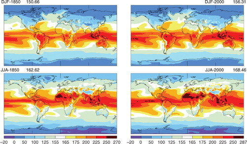
There is more to the greenhouse effect than its global-mean strength and component attribution. Because the greenhouse effect is simply the flux difference between emission by the ground surface and TOA outgoing flux, it is easily calculated from climate model output and displayed in seasonal maps, as shown in Fig. 1. These maps show the space–time variability of greenhouse effect strength, and also provide an opportunity for comparison to observational data.

Fig. 1 Global maps and seasonal change of the greenhouse effect for 1850 (left panels) and 2000 (right panels). The magnitude of the greenhouse effect has increased by about 6 W m⁻² since 1850, but the geographical patterns are largely unchanged. The seasonal change in greenhouse strength (12 W m⁻²) also remains invariant, but it is twice as large as the secular trend. The seasonal change in greenhouse strength is largest over land areas, and it is affected by changes in surface temperature and seasonal shifts in water vapour and cloud distributions. The greenhouse strength is near zero in the Polar Regions, with negative values occurring over Antarctica during the winter season due to large temperature inversions.

Direct comparisons of model-generated greenhouse maps to observational data pose some operational difficulties. There are uncertainties and biases in the available ground-based and microwave sounder unit measurements of surface temperatures (e.g., Trenberth et al., 1992), as well as in the TOA ERBE and CERES flux determinations (Wielicki et al., 1996), and the LW TOA flux reconstructions derived from the ISCCP data analysis (Zhang et al., 2004). Moreover, aside from measurement uncertainties and biases, there are sampling issues and the lack of simultaneity of flux determinations at both TOA and BOA. Nevertheless, the space–time changes in greenhouse strength are quite large, making it practical for useful comparisons with observational data.

The seasonal changes in greenhouse effect strength are driven by the changing solar illumination with latitude. Water vapour and clouds (and atmospheric dynamics) respond rapidly to the changes in solar radiative forcing. Locally, the seasonal changes in the greenhouse strength can exceed 100 W m⁻², with the global-mean G_F increasing by about 12 W m⁻² between the NH winter (DJF) and summer (JJA) months, driven primarily by the large NH continental temperature changes, compared to the less variable SH ocean temperatures.

Compared to the large seasonal changes in greenhouse strength, Fig. 1 also shows the relatively modest changes in greenhouse strength patterns in response to the changes in GHG radiative forcings between 1850 and 2000. This is because the GHG forcing exhibits little change with latitude (e.g., Lacis and Rind, 2013), and also because the GHG forcing is also much smaller than the latitudinal change in solar forcing caused by the seasonally shifting solar illumination.

In regard to the long-term trend, the top-left panel (1850 NH winter with G_F=150.66 W m⁻²) and top-right panel (2000 NH winter with G_F=156.31 W m⁻²), show that the global-mean greenhouse strength increased by 5.65 W m⁻², driven by the 3.1 W m⁻² of radiative forcings coming from non-condensing GHG changes, which are partially counterbalanced by −0.9 W m⁻² of cumulative aerosol forcing over the same time period. By comparison, the corresponding NH summer global-mean greenhouse strength increased by 5.84 W m⁻².

Locally, the greenhouse strength is seen to vary from near-zero values in the polar regions to more than 250 W m⁻² in the tropical convectively active regions. The largest greenhouse strengths are found in those regions with the highest surface temperatures flux (e.g., the Saharan and Australian deserts), and those locations with frequent upper level cloudiness and thus greatly reduced TOA LW flux (e.g., Indonesia). The seasonal and latitudinal changes in greenhouse strength, including their spatial patterns, are prominent features that characterize the changing atmospheric structure in response to the seasonal changes in solar forcing.

The spatial patterns of the greenhouse variability can also serve as important diagnostics of GCM performance. Rather than compare separately maps of surface temperature, water vapour, clouds and TOA LW fluxes (which can cause important correlations and anti-correlations to become obliterated), the greenhouse strength patterns represent an integrated aspect of the radiative and structural effects of the climate variables in a physically self-consistent fashion. The greenhouse strength is in principle an observable quantity – being the difference between the LW flux emitted by the ground and the outgoing LW flux at the top of the atmosphere.

The space–time maps of greenhouse strength in Fig. 1 were obtained from a 5-run ensemble average computed using the GISS 40-layer 2°×2.5° ModelE coupled atmosphere–ocean model with a 32-layer 1°×1.25° ocean model that exhibits El Nino-like variability, and with the full set of radiative forcings from 1850 to 2010. This ModelE version was also used in the CMIP5, Coupled Model Inter-comparison Project.

The global-mean trend in greenhouse strength from 1850 to 2010 shown in Fig. 2 is also from the same 5-run ensemble generated by the coupled 40-layer GISS ModelE. Evident in this trend is the model's ‘natural’ variability due to El Nino-like events, and the clearly identifiable signatures of six major volcanic eruptions from this time period, denoted by the heavy black arrows. These large volcanic eruptions are important climate-forcing experiments that provide important empirical confirmation of the fast-feedback nature of the water vapour and cloud response to radiative forcing changes.

Fig. 2 Time trend of the terrestrial greenhouse effect from 1850 to 2010 from a 5-run ensemble average using the GISS 40-layer 2°×2.5° ModelE coupled atmosphere-ocean model. The 3-D 26-layer ocean model generates El Nino-like inter-annual variability. Also evident are the effects of major volcanic eruptions. These are denoted by the heavy black arrows for the major volcanoes (Shiveluch, Krakatoa, Santa Maria, Agung, El Chichon, Pinatubo). The shape of the greenhouse trend has a strong resemblance to the time trend of the non-condensing greenhouse gases for the same time period.

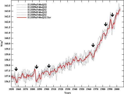
The pronounced global cooling associated with volcanic eruptions is followed by a return to normal after the radiative forcing is gone. This has been noted and analysed by Hansen et al. (1992), Hansen et al. (1996) and Soden et al. (2002), among others. Also of considerable interest is the general shape of the greenhouse strength secular trend and its resemblance to the non-condensing GHG radiative forcing over the same time period.

The LW optical depth of volcanic aerosols, although small in magnitude (Lacis et al., 1992), should act to increase the strength of the greenhouse effect G_F by reducing the outgoing LW flux. However, this increase in greenhouse strength is not observed in Fig. 2. Instead, there are marked reductions in G_F following major volcanic eruptions. This happens because the solar albedo effect of the volcanic aerosol is far stronger than its greenhouse-warming component, causing a decrease in the global temperature and reduction in atmospheric water vapour. This produces dips in global greenhouse strength by as much as 1 W m⁻² following these major volcanic eruptions, providing confirmation of the fast water vapour feedback response.

3. The fast-feedback climate response

The principal source of energy to the climate system of Earth is the Sun (1360.8 W m⁻², Kopp and Lean, 2011). Exhibiting only a ~1 W m⁻² variability over the 11-yr sunspot cycle, solar illumination has been effectively constant over the three decades of precise solar irradiance monitoring. This produces the nominal 240 W m⁻² of solar heating (for a 0.3 planetary albedo), which (all by itself) is sufficient to support a 255K global-mean surface temperature that can sustain a weak water vapour greenhouse effect (as demonstrated in Lacis et al., 2010) commensurate with a snowball Earth climate.

Upon adding the non-condensing GHG greenhouse effect contribution, the energy level at the ground surface is thereby increased by about 38 Wm⁻² (25% of the total greenhouse effect from Table 2). Leveraging this additional heat energy on top of the solar energy enables the Clausius-Clapeyron exponential dependence to bring water vapor and clouds to current-climate levels, which, with a ground level energy at~390 Wm⁻², can sustain the global-mean surface temperature at 288K.

The above is, of course, an oversimplification since energy transactions are not defined at the ground level but rather involve the entire atmosphere. The complexity of the basic processes that are relevant to atmospheric relative humidity structure has been described in Pierrehumbert et al. (2006). What is needed is to determine how, and how fast, the fast-feedback impact takes place within the climate system.

To more clearly illustrate this key point and the nature of the water vapour feedback complexity, we performed two extreme climate-forcing experiments with the GISS ModelE coupled atmosphere–ocean model. In one model run, the water vapour distribution was instantaneously doubled, then allowed to evolve to see if, and how quickly, it would return to its normal equilibrium state.

In the second experiment, GCM's entire the entire water vapor field of the GCM was instantaneously zeroed out, and the model was again allowed to evolve normally. (Actually in this case, we had to settle for reducing the model water vapour by a factor of 1000 to sidestep a divide-check that zero water vapour caused in this version of the model.) However, the net effect was essentially the same, the effective elimination of the radiative forcing due to water vapour at model initialisation.

It can be seen from these ‘water vapour’ experiments that water vapour and clouds are indeed the fast-feedback effects of the climate system. The Clausius–Clapeyron relation sets the equilibrium level for the atmospheric water vapour distribution via the atmospheric temperature structure as defined by solar heating and thermal cooling due to all contributors. Within ~10 d only, water vapour and clouds are back to their normal equilibrium distribution. This is a clear illustration of the fast feedback nature of water vapor and clouds acting as magnifiers of climate change perturbations, but having no lasting impact on the trend direction set by the non-condensing GHGs.

Because water vapour is a strong absorber of thermal radiation, zeroing out the water vapour generates a large initial radiative forcing (from Table 2, a 59.8 W m⁻² cooling effect). Yet within a month of run time, there was no sign of any lasting impact on global climate, with both runs becoming indistinguishable from the control run. In these experiments, because of their large heat capacity, the ocean, land and atmosphere, all retained their equilibrium temperatures. As a result, in the first model time step, water vapour was rapidly evaporating from the ocean to replenish the bone-dry atmosphere. Exhibiting an e-folding time of scarcely more than a couple of days (see bottom-left panel of Fig. 3), water vapour in the lower layers quickly returns to the control run equilibrium distribution. It takes only a little longer for the upper atmospheric levels to reach equilibrium, having to rely on the vertical mixing efficiency of atmospheric dynamics (top-left panel, Fig. 3).

Fig. 3 Hourly model diagnostic results for the ‘virtual’ forcing of climate by instantaneous water vapour changes. There is rapid convergence to equilibrium following instantaneous doubling and zeroing of atmospheric water vapour. The left-hand panels show global-mean water vapour at 299 and 974 mb level converging to control run equilibrium values. The right-hand panels show the upwelling longwave (LW) flux at the top (TOA) and the bottom (BOA) of the atmosphere. Diurnal oscillations in the global-mean LW flux arise from the diurnal surface temperature change over land areas. Red curves depict the model response to doubled water vapour amounts. The green curves refer to the model response to zeroed water vapour. The blue curves are for the control run water vapour reference results. Water vapour changes in the left-hand panels have been normalised relative to the control run results.

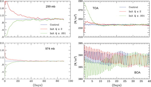
In the complimentary doubling the water vapour experiment, we see an even more rapid return to control run equilibrium, particularly within the lower layers, demonstrating again that the Clausius–Clapeyron equation does not tolerate atmospheric relative humidity in excess of 100% for very long. As water vapour undergoes its rapid transition towards its control run equilibrium, it is affecting the real-time radiative heating and cooling of the atmosphere. The upper-right panel of Fig. 3 shows the changes in the outgoing TOA flux relative to the reference control flux (blue curve). The zeroed water vapour run (green) shows an initial jump (to ~290 W m⁻²) in the outgoing flux because much of the LW thermal opacity was eliminated. As atmospheric water vapour is rapidly replenished, the TOA LW fluxes return to their normal control run level within only a week. There is a small diurnal ripple evident in the TOA LW flux as it converges to its equilibrium value at just less than 240 W m⁻².

The doubled water vapour experiment run exhibits an even sharper response echoing the Clausius–Clapeyron intolerance for relative humidity greater than 100%. Following the initial drop of the TOA LW flux to 220 W m⁻², there is a sharp jump to ~245 W m⁻² that appears to be an over-reaction, very likely related to excess rain-out that caused the TOA LW flux to temporarily exceed the equilibrium level, followed by a more gradual return to equilibrium. The longer period fluctuations of small amplitude appear to be unforced model variability.

The lower right-hand panel of Fig. 3 shows the changes in radiative flux at the bottom-of-the-atmosphere (BOA) due to surface temperature changes in response to the water vapour forcings. Featured prominently is the diurnal cycle of global surface temperature generated by the longitudinal asymmetry in land–ocean distribution. This arises because the land areas are responding to the diurnal shift in solar warming while the Pacific Ocean undergoes only a negligible change in diurnal temperature. Also visible more clearly in the expanded scale, are the uncorrelated natural variability oscillations in BOA LW flux, present in both the control and experiment model runs.

Figure 4 shows the time trend evolution of the greenhouse strength given by the LW flux difference between the BOA and TOA fluxes from Fig. 3. This summarises conclusively the rapid return of global greenhouse strength to equilibrium. There is a sharp drop in greenhouse strength for doubled water vapour from its initial G_F=170 W m⁻² to its equilibrium value of G_F=150 W m⁻². This is to be expected since the doubling of water vapour put many tropospheric grid-boxes above 100% relative humidity, well past the Clausius–Clapeyron saturation limit, causing rapid condensation and rain-out. The large heat capacity of the established thermal structure ensures rapid and unequivocal return to the reference water vapour distribution.

Fig. 4 Hourly model diagnostics of the globally averaged greenhouse effect convergence to equilibrium following the instantaneous doubling (red) and zeroing (green) of atmospheric water vapour. Diurnal oscillations in the globally averaged greenhouse strength result from land-ocean differences in diurnal surface temperature changes. Convergence to equilibrium is fastest for the doubled water vapour experiment since relative humidity above 100% leads to rapid condensation and rain-out. The Clausius–Clapeyron relation is basic to establishing the equilibrium atmospheric water vapour distribution. The reference atmosphere of the time scale zero point is 1 December 1949, which is comparable to the DJF 1850 greenhouse strength in Fig. 1.

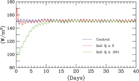
For zeroed water vapor, return to equilibrium is quite fast, but the delay due to the atmospheric transport of water vapor by the dynamic processes is clearly recognizable. Radiative effects of excess or deficit water vapor relative to equilibrium distribution, while real enough, are ‘virtual’ forcings that keep their effect only as long as deviations from equilibrium persist (while the Clausius-Clapeyron constraints act to return water vapor and clouds to their equilibrium level). This describes a climate system that has a well-established equilibrium.

Over-reactions by water vapour and cloud feedbacks will produce ‘virtual’ forcings and unforced variability about the climate system's equilibrium reference point. This may be a contributing factor to the high-frequency ‘weather noise’ of the climate system. On longer time scales, similar fluctuations in ocean circulation will produce ‘virtual’ forcings to which the faster water vapor and cloud feedbacks must also respond. The bottom line is that water vapor and clouds are only within ~10 days from their (temperature based) equilibrium point.

Analysis of the atmospheric relative humidity distribution (Peixoto and Oort, 1996) shows a globally complex but stably structured water vapour field, shaped by atmospheric dynamics and temperature distribution. Water vapour is always striving to reach saturation equilibrium, only to be sharply constrained by rapid condensation when the temperature of atmospheric air parcels exceeds the saturation limit set by the Clausius–Clapeyron equation. Climate change under constant relative humidity was deemed a realistic description of the terrestrial climate system by Manabe and Wetherald (1967). This too is very supportive of the fast-feedback nature of water vapour and clouds, as is exemplified also by the large seasonal changes in greenhouse strength in Fig. 1, and by the diurnal fluctuations in Fig. 4. Radiative modelling aspects of these atmospheric changes are examined in Section 4.

4. Radiative aspects of the greenhouse effect

Modelling thermal radiation is a classical topic that dates back more than a century (e.g., Arrhenius, 1896). Our approach differs from the textbook approach that typically begins with the equation of transfer. We start with Kirchhoff's law and the isothermal cavity concept, which, as illustrated in Fig. 5, leads directly to the expressions for transmission, absorption and emission of LW radiation. These basic formulas are then generalised to model in-layer temperature gradients as shown in Fig. 6. They are then applied to the full atmosphere, which operates basically under conditions of local thermodynamic equilibrium (LTE), as schematically illustrated in Fig. 7.

Fig. 5 Basic principles for transmission, absorption and emission of thermal radiation: Kirchhoff's law of thermal radiation.

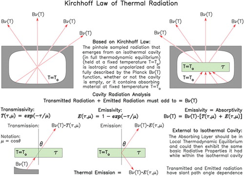
Fig. 6 Thermal emission from homogeneous layer with linear-in-Planck temperature gradient.

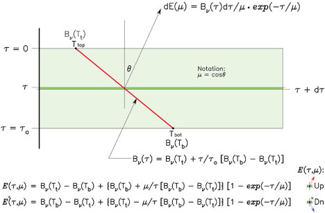
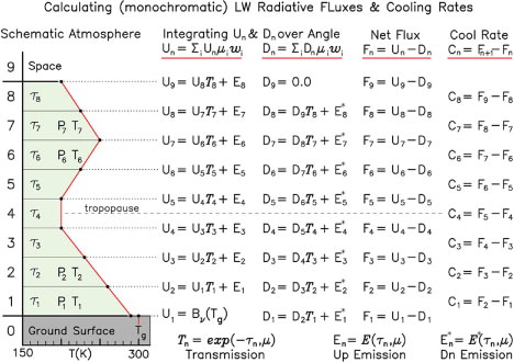
Fig. 7 Schematic outline for computation of monochromatic longwave (LW) fluxes and cooling rates.

Rigorous modelling of thermal radiation involves line-by-line (LBL) methodology, outlined by McClatchey et al. (1972), and used in our radiative transfer modelling, e.g., Lacis and Oinas (1991). The first step is to define the optical depth for each atmosphere layer (the product of the number of absorbing molecules times the absorption cross section per molecule) at each model wavelength, for each molecular absorption line, where the line strength, line width, line energy level and the associated line intensity partition functions are taken from the HITRAN line parameter compilation (Rothman et al., 2009). Here, illustrative calculations are performed using a 40-layer atmosphere with local pressure and temperature dependence for the spectral-line intensity, and with pressure and Doppler (Voigt profile) broadening of spectral-line shape using up to 10⁻⁴ cm⁻¹ spectral resolution. The calculations are made for a clear-sky atmosphere with 1980 level of CO₂, set at 338 ppm.

In our current atmosphere, it is the minor gases, CO₂ (400 ppm) and water vapour (a variable few thousand ppm) that account for the bulk of the atmospheric radiative heating and cooling. Typical lifetimes of LW radiative transitions are of order 10⁻³ s, while typical collision times between atmospheric molecules are of order 10⁻⁷ s. Thus, collisions of air molecules with water vapour and CO₂ molecules exchange heat energy and also serve to establish the LTE population of energy states for water vapour and CO₂ spectral transitions. That is the physical basis for the determination of the spectral absorption cross sections for all the gaseous absorption lines within the HITRAN spectral-line database for the specified atmospheric pressures and temperatures.

The upward and downward directed spectral radiances are calculated as functions of height. Radiances are then integrated over an emission angle to obtain spectral fluxes. Integration over wavelength yields the upward and downward fluxes, which can be differenced to obtain the radiative cooling rate profiles. Radiation is calculated at each grid-box and physics time-step to determine the GCM temperature changes for that time-step.

Discrete layers with linear-in-Planck temperature gradient (Fig. 6) yield analytic expressions for the emitted radiances that are consistent with local thermodynamic equilibrium and the Kirchhoff's law isothermal layer emissivity formulation. This requires far fewer layers to represent the atmospheric temperature profile in calculating the upward and downward directed spectral fluxes (Fig. 7). First, the upward spectral radiances, starting at the ground, are calculated by specifying the Planck spectral intensity for the ground temperature T_g. Model layers are then added, one by one, summing the layer emission plus transmission from below, thus computing the upwelling radiances. Similarly, starting at top, layer emission plus the transmission from above are added layer by layer to obtain the spectral radiances that are incident on the ground.

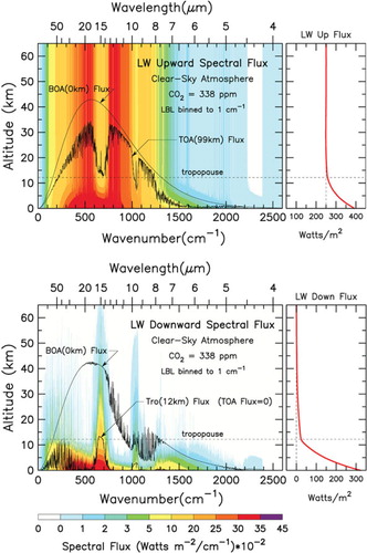
The column spectral radiances are integrated over emission angles using a five-point Gaussian quadrature (Lacis and Oinas, 1991) to obtain the upward and downward directed spectral fluxes, which are depicted in Fig. 8 with colour-proxy height dependence. The radiative fluxes are calculated at layer edges, while the cooling rates apply to the entire layer. LBL results are calculated at 10⁻⁴ cm⁻¹ spectral resolution, and they are binned to 1 cm⁻¹ spectral resolution. The line plots (top panel) depict the Planck spectral flux emitted by the ground, BOA (0 km), and the outgoing flux, TOA (99 km). The bottom panel shows spectral downwelling flux at the tropopause level, Tro (12 km), and the incident spectral flux at the ground level, BOA (0 km). The height dependence of the spectrally integrated upward and downward LW fluxes is shown in the right-hand panels of Figs. 7 and 8. Note that both outgoing TOA and downwelling BOA fluxes originate primarily from within the troposphere. The prominent spectral features that appear in the outgoing TOA flux are the 15 µm CO₂ and the 9.6 µm O₃ bands.

Fig. 8 Upward (top) and downward (bottom) spectral fluxes in clear-sky standard atmosphere.

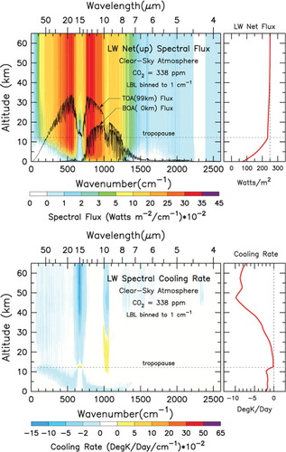
Figure 9 (top panel) shows the spectral net flux for clear-sky standard atmosphere conditions. The top-panel line plots show the net flux at TOA (99 km), and at the ground, BOA (0 km). Notably, virtually all of the cooling by the ground takes place in the LW spectral window. Differencing the net flux yields the LW cooling rate as shown in the bottom panel. Note that most of the stratospheric cooling occurs within the 15 µm CO₂ band, with substantial contributions also from the 9.6 µm O₃ band and the water vapour rotational band. In the troposphere, it is water vapour that is the principal radiative cooling agent.

Fig. 9 Clear-sky case spectral net flux (top panel) and spectral cooling rate (bottom panel).

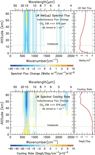
Figure 10 (top panel) shows the instantaneous spectral net flux change for doubled CO₂ (338–676 ppm). The right-hand panel depicts the spectrally integrated instantaneous net flux change with height (the negative of the instantaneous radiative forcing), which for the clear-sky case, is about 5 W m⁻² at the tropopause. The instantaneous spectral cooling rate due to doubled CO₂ is shown in the bottom panel. Note the strong upper stratospheric cooling in the 15 µm band, with smaller contributions from lesser CO₂ bands. A small warming in the troposphere is also contributed by the 15 µm CO₂ band.

Fig. 10 Spectral net flux change (top) and spectral cooling (bottom) for doubled CO₂.

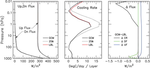
LBL calculations are the standard against which radiative modelling results are compared. Although computer capabilities have increased greatly over past decades, LBL calculations remain too costly for climate GCM applications. Nevertheless, much of the LBL numerical precision can be reproduced in GCM-type radiation models by utilising the correlated k-distribution approach (Lacis and Oinas, 1991) to model the gaseous absorption in vertically inhomogeneous atmospheres. Figure 11 shows illustrative comparisons between LBL-calculated results and the GISS ModelE radiation code, which reproduces the LBL accuracy to within ~0.1% under typical current climate atmospheric conditions.

Fig. 11 Line-by-line (LBL) and 3-D general circulation climate model (GCM) radiative flux and cooling rate comparisons for Mid-Latitude Atmosphere calculations. Reference LBL calculations are depicted in red. GISS ModelE calculations using the correlated k-distribution methodology are plotted in black (on top of the red lines). Left-hand panel shows virtual agreement for the downwelling and upwelling fluxes. Cooling rates are shown in the middle panel, with flux differences plotted at right. The 33 spectrally non-contiguous correlated k-distribution intervals in the GCM radiation model are able to closely reproduce the LBL calculation results that utilise over 10⁷ spectral points. For comparison, the dotted lines depict the corresponding results for the vintage 25-k interval GCM radiation model from Hansen et al. (1988), which is used in the climate-forcing calculations for extreme CO₂ amounts described in Section 6.

Radiation is the key process within the climate system that regulates the energy balance of the Earth, implying detailed balance between solar and thermal radiative fluxes. While the focus in this study is on the treatment of thermal LW radiation, evaluating LW radiation effects must be done in conjunction with the solar SW radiative effects arising from water vapour, clouds, aerosols, ozone and other absorbing atmospheric gases. The accuracy for treatment of solar SW radiation in ModelE is comparable to the treatment for thermal radiation (Hansen et al., 1983; Schmidt et al., 2006). This is achieved by adapting the doubling-adding method for modelling multiple scattering (Lacis and Hansen, 1974), and by adapting the correlated k-distribution methodology to model SW gaseous absorption.

To adequately incorporate the role of clouds in climate, it is necessary to have a physically self-consistent treatment of cloud radiative properties over both the SW and LW spectral regions. To this end, accurate modelling of cloud and aerosol radiative effects makes full use of spectrally dependent (and spectrally resolved) Mie scattering cloud (and aerosol) radiative parameters across the entire SW and LW spectral regions.

Thermal LW radiation determines how the greenhouse effect keeps the surface temperature of the Earth some 33K warmer than it would otherwise be if there was no thermal opacity in the Earth's atmosphere. The basic principle of the terrestrial greenhouse effect is that the non-condensing GHGs (utilising absorbed solar radiation) provide the temperature structure that sustains the water vapour and cloud distributions in the atmosphere under the control of the Clausius–Clapeyron equation. For current climate, water vapour and clouds account for ~75% of the total greenhouse strength but are acting as temperature-dependent feedback contributors. Accordingly, water vapour and clouds can only magnify the radiative effect of the non-condensing GHGs. This reality makes CO₂ the principal control knob that actually governs the global surface temperature of Earth, even though CO₂ by itself accounts for only about 20% of the total greenhouse strength.

The controlling role of atmospheric CO₂ is demonstrated further in the next section in the context of the geological ice-core record (Fig. 12) where changes in CO₂ (and CH₄) are seen to occur in lock-step with global ice-age events. The intrinsic control-knob nature of atmospheric CO₂ is made more telling in Fig. 13, as CO₂ is varied from near zero to large extremes.

Fig. 12 Geological record of climate forcings, temperature, sea level and surface albedo response. (a) CO₂ and CH₄ data are derived from the Antarctic Dome C ice-core analysis, sea-level record based on analysis of Bintanja et al. (2005). (b) Greenhouse gas and surface albedo forcing are from GCM modelling studies, with ice sheet area inferred from sea-level changes. (c) Dome-C-derived temperature change has been divided by two to represent global-mean temperature change. The calculated temperature change is based on a fast-feedback climate sensitivity of 0.75°C per W m⁻², as per 3°C for doubled CO₂. (after Hansen et al., 2008)

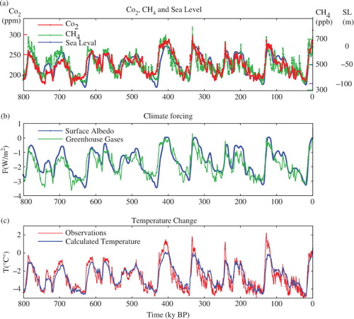
Fig. 13 Global energy balance analysis using global equilibrium surface temperature comparisons over an extended range of CO₂ radiative forcing. At the left is the energy input scale (W m⁻²) with red arrows designating solar energy input. Heavy blue arrows represent outgoing energy [reflected solar, and longwave (LW) TOA flux to space]. The temperature scale in the figure interior gives the surface temperature (°C). The right-hand scale is for effective temperature (K). The pink region, covering the range of successive CO₂ doublings, is the absorbed solar radiation (W m⁻²). The green region represents the radiative forcing caused by the successive CO₂ doublings. The yellow region depicts the water vapour and cloud fast-feedback contribution (W m⁻²) to the total greenhouse strength. At bottom right, minor non-solar sources of energy input to the global climate system are shown in equivalent effective temperature units. The heavy red arrow angling towards figure top depicts a possible ‘runaway’ danger zone where positive CO₂ feedbacks from existing CO₂ reservoirs have the potential to exceed human capacity to maintain control over global climate change. Model results were calculated using the Russell et al. (2013) 27-layer, 4°×3° coupled fast atmosphere-ocean model (FAOM). Based on attribution analysis, the feedback contribution to the greenhouse strength (yellow) is subdivided into its water vapour and cloud components. Similarly, the radiative forcing contribution to the greenhouse strength (green) is subdivided into CO₂ and other GHG contributions. Similarly, the absorbed solar radiation (pink) is subdivided into portions that are absorbed within the atmosphere and solar radiation that is absorbed by the ground surface. The Effective Temperature and Surface Energy scales coincide numerically at zero, and also at the common point where 260.3 K=260.3 W/m², connected otherwise by slanted lines.

5. Geological perspective and context

In Fig. 12, the geological comparisons over 800000 yr of the ice-core data record provide an independent check on the fast-feedback climate sensitivity and confirm the basic self-consistency of a climate sensitivity of 3°C for doubled CO₂ over a broad range of CO₂ concentrations, albeit not for the much higher levels of CO₂ that are currently encountered in the atmosphere or are being anticipated in the years to come.

As described in Hansen et al. (2008), the sources and sinks of CO₂ on geological time scales are not generally in balance at any given time. The principal source of atmospheric CO₂ is volcanic activity, while chemical weathering of rocks is the principal sink, slow processes that redistribute CO₂ at a rate of about 10⁻⁴ ppm yr⁻¹, compared to present human-driven rate of approximately 2 ppm yr⁻¹. During glacial-interglacial periods shown in Fig. 12, the typical rates of CO₂ change are within the range of 10⁻² to 10⁻³ ppm yr⁻¹, due to still poorly understood biological and ocean chemistry processes that are ultimately driven by the slow changes in the Earth's orbital parameters. These slow CO₂ changes on geologic time scales are effectively an imposed climate forcing, while the glacial–interglacial CO₂ oscillations are a slow feedback response to climate changes forced by orbital changes. In both cases, the CO₂ changes are the key radiative forcings that drive further water vapour and cloud feedbacks. In this way, CO₂ controls the global temperature over geological time scales. Radiatively, CO₂ and CH₄ are similar, but CH₄ is less important because its principal LW spectral band is much narrower than that of CO₂, and its atmospheric residence time is only about a decade.

A fast-feedback sensitivity of about 3°C for doubled CO₂ is implied by the interglacial temperature variation. There is an additional 3°C climate sensitivity for the slow (ice sheet) surface albedo feedback processes. This is consistent with the fast-feedback sensitivity in current climate GCM simulations for doubled CO₂, and which is also inferred and supported by the greenhouse flux attribution analysis. Still, as noted by Aires and Rossow (2003), climate feedback sensitivity in non-linear systems is state dependent, and not some fixed constant of the climate system. The 3°C sensitivity for doubled CO₂ fits both current climate and the geological record in a broadly general sense. Evidence that climate sensitivity does undergo change with changing climate is demonstrated in the next section.

6. How CO₂ controls global climate change

The pivotal role of CO₂ as the LW control knob of global climate is demonstrated in Fig. 13 by varying atmospheric CO₂ from 1/8 to 256 times the nominal 310 ppm 1950 CO₂ amount, causing the terrestrial climate to change from a frozen snowball Earth to life-intolerable hot-house conditions, all derived from climate GCM simulations. The left-hand surface energy scale depicts the thermal heat energy that is available at the ground surface to drive atmospheric winds and weather events and to sustain water vapour and clouds distributions, which actually are by far the largest contributors to the strength of the terrestrial greenhouse effect. The global-mean surface temperature is the one physical parameter that characterises best the habitability prospects of the biosphere over the extreme range of global climate change seen in Fig. 13. The surface temperature (°C) scale near figure centre is linearly aligned with the right-hand (°K) effective temperature scale, and it is connected by the slanted lines to the corresponding surface energy scale (W m⁻²) values on the left. The objective is to depict clearly the σT⁴ dependence between energy and temperature.

It is the temperature dependence of the Clausius–Clapeyron equation that acts to both sustain and constrain the water vapour distribution in the atmosphere, leading to cloud formation and precipitation whenever relative humidity exceeds 100%. The energy that is available to the climate system consists of the absorbed solar energy (the light and darker pink areas), the greenhouse effect thermal energy (yellow and green areas), as well as several sources of non-solar energy (i.e., geothermal, tidal, and waste heat) that are of negligible magnitude when compared to the solar and greenhouse thermal energies, and are too small to be visible on the energy scale. There is also a large store of latent heat potential energy (not shown) that can energize extreme weather events when released. Its averaged effect acts to maintain the atmospheric temperature structure.

Figure 13 summarises the response of the SW and LW energy components of the terrestrial climate system to large changes in radiative forcing, showing how the incident solar radiation is partitioned between reflected and absorbed components, and how this partitioning changes under different climate regimes. Of special note is the growing strength of the greenhouse effect as atmospheric CO₂ changes from near-zero to extreme values, highlighting the controlling nature of CO₂ forcing.

6.1. Solar energy input to climate system

The solar energy available to the terrestrial climate system is 341.5 W m⁻² (in FAOM runs, S₀=1366 W m⁻²). The Sun has been a very stable source of energy, exhibiting only about a 0.1% oscillation over the 11-yr solar sunspot cycle. In the geological context, solar luminosity has gradually increased from its initial 240 W m⁻² of incident solar energy 4.5 billion yr ago (dashed red arrow at left in Fig. 13) – as a result of hydrogen conversion to heavier elements in the solar interior (Sackmann et al., 1993). Of the incident solar radiation, about 106 W m⁻² are reflected back out to space by clouds, ground surface and by molecular scattering by air, leaving 235 W m⁻² as the (global-mean) external input of solar energy to the climate system (for the FAOM planetary albedo of 0.31).

6.2. Non-solar energy input to climate system

The principal sources of non-solar energy input are shown at the bottom right of Fig. 13. These are geothermal, waste heat (e.g., nuclear, fossil fuel combustion) and tidal energy. Globally averaged, geothermal energy, at 0.092 W m⁻², is the largest of the non-solar energy sources. Waste heat generated by nuclear energy and the burning of fossil fuel contributes 0.028 W m⁻², while tidal energy contributes a mere 0.006 W m⁻². Although they can be significant as local-level sources of heat energy, they are negligible when compared to the uncertainty in the 235 W m⁻² of global solar radiation input. If the Earth had no energy source of its own, its surface temperature would be in equilibrium with the 3K cosmic background temperature. If the Earth was limited to only its non-solar energy sources, the Earth could muster a surface temperature of about 38.6K, which is colder than the 44K surface temperature on Pluto. Because of their miniscule magnitude and limited variability, these non-solar energy sources are typically not included in climate simulations. Their presence becomes noticeable only when compared as an effective temperature relative to absolute zero (0K), as shown in the lower right corner of Fig. 13.

6.3. Global energy balance/surface temperature

All by itself, the 235 W m⁻² of absorbed solar energy (for the FAOM 0.31 planetary albedo) is sufficient energy to sustain a global-mean surface temperature of the Earth of about 254K (−19°C). However, this amount of heat is still far too cold for the Clausius–Clapeyron relation to support more than a small amount of water vapour in the atmosphere (about 10% of the current climate value, which is incapable of raising the global surface temperature above freezing). Therefore, an additional source of heat energy is required within the climate system (such as the increased warming generated by the greenhouse effect due to the non-condensing GHGs) – one that can support atmospheric water vapour at a level where the additional water vapour thermal opacity can contribute toward maintaining the temperature structure needed to sustain the biosphere.

Solar energy is of course being absorbed both at the ground surface and throughout the entire atmosphere. But given that the strength of the greenhouse effect (G_F) is defined as the LW flux difference between the flux emitted by the ground surface (F_GS) and outgoing TOA flux (F_LW), it is convenient to think of F_GS (a proxy for the surface temperature) as being composed of the greenhouse strength term plus the absorbed solar energy, because F_SWa is equal to F_LW when the Earth is in radiative energy balance (i.e., F_GS=G_F+F_SWa). Since the temperature at the ground surface is also the point of maximum temperature within the biosphere, this can serve additionally as a useful indicator of global habitability conditions.

Given that the Earth's global energy balance at TOA is characterised by radiative transfer means only, detailed radiative attribution analysis can be performed on the model-generated global temperature, water vapour and cloud distributions. The effects of dynamical heat transport, energy conversion, as well as land–ocean–atmosphere heat capacity interactions get fully incorporated within the model-generated temperature–absorber distributions. Therefore, the global surface temperature dependence on changes in atmospheric absorber distribution can be inferred from radiative modelling analysis of the changes in the SW and LW global energy balance.

6.4. Control run setup

The GCM climate change simulations in this study utilise the 27-layer, 4°×3° fast atmospheric–ocean model (FAOM) with a 100-m ocean (Russell et al., 2013) using the Arakawa and Lamb (1977) C-grid numerical scheme, and a step-mountain technique to improve model performance (Russell, 2007). The treatment of model dynamics, moist convective and radiative processes is similar to those in the GISS ModelE (Schmidt et al., 2006), though not identical, particularly the treatment of clouds, which is more simplified here than in ModelE.

In general, FAOM clouds are set when local temperature and the water vapour distribution exceed the relative humidity condensation criteria (as dictated by the Clausius–Clapeyron relation). The cloud treatment is basic in the sense that cloud optical depth is set to be proportional to the condensable water amount, with the cloud particle size held fixed at an effective radius of 10 µm. If the local temperature is less than 0°C, ice clouds are formed with an (equivalent sphere) effective radius of 25 µm. The cloud optical depth proportionality coefficient and effective relative humidity condensation point are model parameters that cannot be determined from first principles. These model parameters are ‘empirically’ adjusted so as to reproduce the observed current climate conditions. In this way, the FAOM has a global planetary albedo of 0.31, global-mean surface temperature near 15°C, with sea-ice extent, water vapour and cloud distributions that are closely representative of current climate conditions. FAOM uses 1366 W m⁻² for S₀. The 100-m ocean underestimates ocean heat transport, but it does permit rapid global temperature and energy convergence to equilibrium in less than a century (Russell et al., 2013).

6.5. Radiative forcing

The radiative forcing in Fig. 13 is specified by the change in atmospheric CO₂ expressed as 2^N×CO₂, where N ranges from −3 to 8, or from 1/8 to 256 times the 1950 CO₂ amount. The incremental CO₂ change is specified in ppm, which is then converted to W m⁻² by the GCM radiation model. Radiative fluxes are calculated in the context of the local atmospheric temperature, water vapour and cloud distributions to obtain the atmospheric heating and cooling rates that drive atmospheric motions. This radiative forcing produces a temporary global energy imbalance at TOA, which also makes it an effective indicator of the magnitude of the radiative forcing that drives the climate system towards its new equilibrium.

The formula derived in Hansen et al. (1988) provides an estimate of ~4 W m⁻² for the initial radiative forcing at the tropopause for each doubling of CO₂. As the climate warms (or cools) in response to the applied initial radiative forcing, the radiative flux imbalance diminishes as feedback processes interact to bring the atmospheric distribution of water vapour, clouds and temperatures to their new equilibrium distribution. As has been pointed out by Aires and Rossow (2003), in a non-linear climate system, not only the feedbacks, but also the radiative forcings are state dependent. They evolve gradually as the climate system changes. Additional perspective on the evolving relationship between radiative forcing, feedback and climate sensitivity emerges from the greenhouse attribution analysis described in Section 2 (and illustrated in Fig. 13) for model runs with specified CO₂ concentrations, where each of the 12 FAOM-modelled CO₂ radiative forcing experiment runs are individually time-marched to global equilibrium.

6.6. Forcing and feedback attribution

Attribution quantifies the relative importance of the different atmospheric constituent contributions to the greenhouse effect. The non-condensing GHGs (CO₂, CH₄, N₂O, O₃, CFCs) are readily identified as the ‘radiative forcings’ of the climate system. This is because once they have been injected into the atmosphere, they remain there for decades (or centuries, as is the case for CO₂ and CFCs), subject only to slow chemical removal processes. However, water vapour and clouds are ‘feedback effects’ since their equilibrium distributions are directly dependent on local atmospheric temperature structure (as demonstrated in Section 3). Hence, (at least on time scales that are relevant to current climate) there is a clear distinction as to which climate constituents act as climate system forcings (the non-condensing species), and those that behave as climate feedbacks (water vapour and clouds).

The term ‘radiative forcing’ typically refers to the radiative flux imbalance at the tropopause caused by a change in some radiative forcing constituent. The greenhouse flux attribution gives a different perspective that takes into account the entire atmospheric thermal structure. For current climate conditions, this structural radiative effect is summarised in Table 3. It shows non-condensing greenhouse gases accounting for ~23% of the greenhouse effect (~18% for CO₂ and ~5% for CH₄, N₂O, O₃, CFCs combined). Water vapour and clouds account for ~77% of the greenhouse effect, implying a ‘structural feedback’ sensitivity, f=4.4 Attribution numbers for snowball Earth conditions (1/8×CO₂) are: ~76% feedback and ~24% forcing, with f=4.15. For 256×CO₂, the greenhouse strength attributions produce: ~86% feedback and ~14% forcing, with f=7.14. The corresponding changes in the greenhouse flux, G_F, are 42 W m⁻² for 1/8×CO₂, 156 W m⁻² for 1×CO₂ and 440 W m⁻² for 256×CO₂, respectively.

Table 3. LW greenhouse effect (G_F) fractional attribution

Component	1/8×CO2	1×CO2	256×CO2
Water vapour	0.409	0.548	0.701
Cloud	0.350	0.224	0.159
CO2	0.221	0.179	0.106
Other GHGs	0.020	0.049	0.034
Total GF (W m^−2)	42.25	156.44	439.61

GHG, greenhouse gas; LW, longwave.

The attributed changes in water vapour and cloud feedback are represented by the yellow coloured area in Fig. 13, with the dotted line separating the water vapour and cloud contributions. Similarly, the radiative forcing caused by the non-condensing GHGs is depicted by the green coloured area that is subdivided into the CO₂ and other GHG fractions, which are delineated by the light dotted line. The magnitude of forcing by the minor GHGs (CH₄, N₂O, O₃, CFCs, denoted as GH_x) increases slowly from left to right in Fig. 13 because of changing atmospheric temperature structure, even though the atmospheric concentration of these gases is kept constant. Because of this, as seen from Table 3, the GHx relative fractional contributions to the greenhouse strength show some variability, as seen from Table 3. The CO₂ structural forcing also increases steadily from left to right in Fig. 13, but not at the incremental ~4 W m⁻² rate of the initial radiative forcing expected for each CO₂ doubling. This is because of the ever-changing atmospheric temperature–absorber distribution, and also because of the strong spectral overlap of H₂O and CO₂ absorption, where the rapidly increasing water vapour opacity overwhelms the more saturated CO₂ forcing.

Table 4 lists the fractional attributions for the reflected and absorbed components of solar radiation. Though the reflected SW components are not explicitly quantified as such in Fig. 13, they are contained within the light blue area, which is blocked in part by the green and yellow greenhouse effect components. It is located between the heavy dashed 341.5 W m⁻² incident solar radiation line and the heavy red speckled line that defines the total solar SW radiation absorbed by Earth. This depicts the full conservation of energy for the incident solar radiation – delineating the fraction reflected and the fraction absorbed, specifying also where the solar radiation is absorbed.

Table 4. SW solar reflected/absorbed fractional attribution

Reflected SW	1/8×CO2	1×CO2	256×CO2
Cloud	0.229	0.595	0.575
Rayleigh	0.062	0.140	0.195
Surface	0.709	0.265	0.230
SW refl (W m^−2)	180.43	106.02	79.83
SW refl (%)	52.83	31.05	23.38
Absorbed SW
Water vapour	0.091	0.185	0.206
Gases and clouds	0.215	0.111	0.076
Surface	0.694	0.704	0.718
FSW (W m^−2)	161.07	235.48	261.67
SW abs (%)	47.17	68.95	76.62

SW, shortwave.

In Table 4, the SW solar radiation reflected by the Earth (planetary albedo) is 53%, 31%, 23% for 1/8×CO₂, 1×CO₂, 256×CO₂, respectively. As expected, for the snowball Earth conditions, most of the reflected radiation (71%) is reflected by snow/ice of the ground surface. For current climate 1×CO₂ conditions, clouds are responsible for approximately 60% of the reflected radiation, with decreasing cloud contributions towards both warmer and colder climates. Rayleigh scattering is effectively an invariant radiative scattering constituent, but its relative fractional importance is seen to change substantially as the result of shifting competition with snow/ice and cloud scattering effects.

Attribution of the absorbed solar SW radiation is shown in Fig. 13 by the pink areas. The darker pink region depicts the fraction of the incident solar radiation absorbed by the ground surface, while the lighter pink area depicts the fraction that is absorbed within the atmosphere. Notably, relative partitioning (30% vs. 70%) between the atmosphere and ground absorption appears not to vary significantly over the entire range of CO₂ forcing. Except under snowball Earth conditions (when ozone absorption dominates), water vapour is the dominant absorber of SW solar radiation, becoming increasingly more dominant as climate continues to get hotter.

With the current climate atmosphere as the reference point, the implied ‘structural feedback’ sensitivity, f=4.4, is defined by the ratio (yellow+green)/green, or the sum of water vapour, cloud and non-condensing GHG fluxes divided by the non-condensing GHG radiative forcing. In principle, this is a quantity that is empirically verifiable. If the model-generated water vapour, cloud and temperature distributions are a close match to observational data, performing flux attribution on model-generated and observed data should yield similar values for the climate feedback sensitivity - ones based on the overall temperature–absorber structure of the climate system. As noted in Section 2, since flux attribution is performed for a fixed temperature structure, the structural feedback sensitivity does not include the negative lapse rate contribution that would be a part of the climate feedback sensitivity for perturbations that are made relative to current climate such as doubled CO₂.

In a somewhat broader perspective, the climate system's overall ‘forcing-feedback efficacy’ factor f can be defined as6

where F_GS is the global-mean LW flux emitted by the ground surface (proxy for surface temperature via ), and where F_SWi=S₀/4 is the global average annual-mean incident solar flux. Analogous to the analysis of Hansen et al. (1984), the LW surface flux can be expressed as7

where (via attribution) and ΔF_GHG are the greenhouse fluxes due to CO₂ and other non-condensing GHGs (the green coloured ‘forcing’ areas), where and ΔF_CLD are the greenhouse fluxes due to water vapour and clouds (the yellow coloured ‘feedback’ areas), and where ΔF_ALB is the solar radiation that is reflected back to space. Dividing eq. (7) by F_GS and substituting for F_SWi/F_GS from (6) yields8

where the flux ratios (e.g., /F_GS, ΔF_GHG/F_GS) are the relative feedback efficacy gain factors for the specified climate system processes. The specific flux contributions for each component are found via the flux attribution analysis as outlined in Section 2. The term ΔF_ALB/F_GS is negative since it takes energy out of the climate system by reflecting it back to space. In this perspective, it is solar energy (which has been remarkably constant over past decades) that is the ultimate external forcing of the climate system. All else is Planck and dynamical response to internally imposed forcings (e.g., non-condensing GHGs and volcanic aerosols) and internally induced feedbacks (water vapor and clouds) that generate the radiative impetus to drive the climate system toward a new energy balance equilibrium.

Changes to the LW flux emitted by the ground surface, F_GS, stem from the Planck response to the absorbed solar radiation and from the changes in greenhouse structure initiated by the changes in radiative forcing constituents. In this perspective, the only thing that differentiates radiative forcings from the radiative feedbacks as to their contributions to the greenhouse effect and to the global surface temperature is only the happenstance that the non-condensing GHG distributions do not depend on temperature, while both water vapor and cloud distributions are interactively dependent on the local temperature.

In comparing two equilibrium climate states, for example, current climate and doubled CO₂, differencing of eq. (7) would yield the radiative forcing term and the feedback terms and δF_CLD. There would also be the albedo term δF_ALB incorporating cloud albedo and surface albedo contributions, and a small change in δF_GHG (due to atmospheric structural changes, even though the GHG amounts remain unchanged), as well as a negative feedback term due to temperature lapse rate change between the two equilibrium climate states.

Overall, the radiative flux attributions can be rigorously calculated for all contributors (see Section 4). From this it follows that the imposed radiative forcings will be robustly quantified since the changes in non-condensing GHGs are accurately known, and are not affected by transient changes in climate. Water vapour and cloud feedback terms, however, are subject to more uncertainty since the distribution of atmospheric water vapour is strongly affected by stochastic changes in atmospheric dynamics even though the Clausius–Clapeyron constraint itself is sufficiently precise. Meanwhile, the cloud feedback terms are subject to even larger uncertainty since in addition to local atmospheric dynamics effects, cloud properties such as optical depth, particle size and cloud cover are also uncertain, and are in need of improved physical models.

The climate system's ‘forcing-feedback efficacy' factor f (G_F from Table 3+F_SW from Table 4, divided by 341.5 W m⁻²) varies from f=0.6 for snowball Earth conditions, to f=1.15 for current climate Earth, to f=2.05 for the 256×CO₂ extreme. For reference, f=1 for a completely absorbing planet without a greenhouse effect, while f=0 for a completely reflecting planet. Thus, f is simply the efficacy coefficient that defines how effectively incident solar energy heats the ground surface. It describes the greenhouse effect response to the non-condensing GHGs, magnified by feedback changes in water vapour and cloud, and counterbalanced by the cloud, surface and Rayleigh scattering effects. Although not specifically identified as an energy term in Fig. 13, the latent heat energy generated by the increase in water vapour is a potent form of potential energy that is released when water vapour condenses. This additional available energy provides more fuel for increased frequency and/or severity of weather extremes with continued global warming.

6.7. Water vapour feedback response

The atmospheric distribution of water vapour is subject to the exponential Clausius–Clapeyron temperature dependence that effectively doubles the water vapour amounts for every 10°C increase in temperature. However, the other factors that affect the atmospheric water vapour distribution are more complex. These include the energy that is available at the ground surface for evaporation, the dependence of evaporation on wind speed, near-surface turbulence, transport though the boundary layer, as well as vertical and horizontal transports in the atmosphere with condensation, precipitation and re-evaporation all taking place along the way. All of these factors need to be explicitly modelled in GCM simulations, comprising a likely source of uncertainty - but one where model performance can be verified by comparing seasonal and regional-model-generated water vapour distributions against observational data.

Despite the complexity, there is convincing evidence that the relative humidity tends to remain relatively constant as climate changes (e.g., Held and Soden, 2000). There is also evidence for enhanced upper tropospheric humidification in a warming climate, as described in the early climate feedback sensitivity studies (Hansen et al. 1984). Efficacy of water vapour as a GHG becomes greater with height, peaking in the 15–20 km altitude region (e.g., Rind and Lacis, 1993), which is one important aspect of the growing water vapour feedback contribution to the growing greenhouse effect. There is also a large negative feedback component associated with changing water vapour. This is the moist adiabatic lapse rate feedback that is negative in the tropics and becomes positive in the polar regions.

It is expected that some of the effects of the exponential increase in water vapour might be compensated by logarithmic saturation. While some parts of the water vapour spectrum are indeed logarithmically saturated, water vapour has numerous weak lines across the spectrum that are far from saturation and would tend to absorb linearly. Also, the self-broadened water vapour continuum absorption in the LW spectral window region increases as the square of the water vapour density (Baranov et al., 2008).

One reason for the growing strength of the water vapour greenhouse efficiency is the increase in the upper tropospheric relative humidity. This tendency is propagated upward into the stratosphere (Russell et al., 2013) where local heating by the additional water vapour tends to eliminate the tropopause cold trap (evident at 8×CO₂), which opens the door for more water vapour to be transported into the stratosphere.

Water vapour is the strongest greenhouse contributor of the climate system feedback process, and its dependence on the well-established Clausius–Clapeyron relationship commands a considerable robustness. Still, the uncertainties associated with parameterisations of the vertical and horizontal water vapour transport, evaporation and rain-out may induce biases in the overall strength of the water vapour feedback effect. This may account for the FAOM fractional water vapour greenhouse contribution obtained for 1×CO₂ in Table 3 being larger than the GISS ModelE result in Table 2.

6.8. Cloud feedback response

Similar to water vapour, clouds are also closely constrained by the Clausius–Clapeyron relation but with greater cause for uncertainty. With no cloud microphysical model available to calculate cloud properties from first principles, the modelling approach is to set the cloud optical depth in proportion to the condensable water amount. This way, the cloud optical depth coefficient and the effective relative humidity condensation point can serve effectively as model ‘tuning’ parameters that can be ‘empirically’ adjusted to reproduce the current climate conditions, namely, a global planetary albedo near 0.30, global-mean surface temperature near 15°C, including the observed sea-ice extent and water vapour and cloud distributions.

In this study, there is greater climate feedback sensitivity in going towards both colder and warmer climate, a characteristic that was found earlier by Hansen et al. (2005). In going towards colder climate, there is a tendency for the low cloud cover to increase, as might be expected from the Clausius–Clapeyron temperature response. This cloud cooling effect is amplified by the Clausius–Clapeyron constrained decrease in atmospheric water vapour, and by the strengthening of the snow/ice albedo feedback, especially when global climate is heading towards snowball Earth conditions. The effect of increased low clouds going towards a colder climate causes reflected solar radiation to increase, while reflection by the middle and high clouds tends to decrease. But, in approaching snowball Earth climate conditions, the rapid increase in snow/ice cover overwhelms the cloud contribution to the planetary albedo.

In going towards a warmer climate, the increased surface heating tends to diminish the low cloud cover (e.g., Hansen et al., 1997). Also, there is a growing tendency for clouds to form at higher altitude as the climate warms, which has the effect of increasing their greenhouse efficacy because of the growing temperature differential between the cloud radiating-to-space level and ground. In going from current climate (66% cloud cover) to 256×CO₂ (30% cloud cover), there is also a shift of clouds moving towards higher latitudes, making the clouds less efficient in reflecting solar radiation since most of the solar radiation falls on tropical latitudes. This is corroborated by the steady increase in absorbed solar radiation (the heavy red speckled line in Fig. 13) as CO₂ increases from 1/4 to 8×CO₂.

Noticeable transitions occur in the cloud feedback effect. A sharp transition is encountered from 1/4 to 1/8×CO₂ as the snow/ice feedback becomes dominant. A subtle shift in slope occurs at 8×CO₂ when the tropopause becomes obliterated by increasing water vapour opacity, allowing transport of more water vapour into the stratosphere. At 32×CO₂, there is an apparent flattening of the absorbed solar radiation slope, and a decrease at 256×CO₂. In all these cases, there is a continued decrease in cloud cover with a partially compensating increase in cloud optical depth, one which is not sufficient to produce an increase in planetary albedo, except for 256×CO₂ where a large increase in low cloud optical depth occurs. However, in this case, the ‘low’ clouds now occur at altitudes above 10 km.

Overall, the global cloud changes that occur as CO₂ forcing is varied from snowball Earth to hot-house conditions, appear plausible, given the water vapour, temperature and dynamical changes that take place. However, with no microphysical cloud model against which to evaluate the cloud changes, the cloud changes so incurred could well be artefacts of parameterisation, able to simulate current climate conditions, but not have the predictive capability for large departures from current climate. Nevertheless, even though the cloud feedback treatment might be suspect, this has little impact on the overall CO₂ greenhouse effect analysis because to a large extent the cloud SW albedo and LW greenhouse effects counteract each other (see Fig. 13). Although the precise degree of cancellation remains a key research question for current climate feedback sensitivity, the net effect is that water vapour changes (which are more strongly constrained by the Clausius–Clapeyron relation) will dwarf the uncertainties that may arise from poor cloud treatment.

Still, given the 2% decrease in cloud cover for doubled CO₂, it is likely that the FAOM cloud treatment supports cloud feedback that is too strongly positive. Coupled with the larger snow/ice feedback that is incurred by using the 100 m ocean, this could account for the FAOM sensitivity to doubled CO₂ of 4.9°C being at the high end of the nominal IPCC range for doubled CO₂ equilibrium response of 3.2±1.2°C (Meehl et al. 2007). Meanwhile, as partial compensation, the FAOM tends to underestimate the strength of the greenhouse effect by several W m⁻² because FAOM uses the older 25-k interval radiation model instead of the 33-k ModelE version (Oinas et al. 2001). As shown in Section 4, the 33-k interval treatment reproduces stratospheric radiative transfer more accurately.

6.9. Geophysical perspective and relevance

The heavy red arrow angling upward toward the top of Fig. 13 describes a potentially catastrophic climate calamity that lurks within the realm of future climate scenarios, a looming threat menacing the habitability of Earth. The extreme atmospheric CO₂ amount that is represented by the 256×CO₂ example is far in excess of the carbon that is available as fossil fuel. But approaching 4×CO₂ is a prospect that is within reach if the current rate of fossil fuel use continues into the next century.

The problem of concern is that there are large reservoirs of CO₂ – the ocean, permafrost, biosphere and soil, including also the large, but uncertain, amounts of CH₄ that reside in methane clathrates. Because these large reservoirs of carbon are temperature dependent, and because global temperature is being driven ever higher by the continued burning of fossil fuel, there is increasing risk that these carbon reservoirs may start to emit significant amounts of CO₂ into the environment (as a positive CO₂ feedback effect).

If at some point, the combined rate of CO₂ emission into the atmosphere due to continued fossil fuel burning and CO₂ reservoir outgassing (including a reduced or reversed ocean uptake of CO₂) begins to exceed the human capacity to control the input of CO₂ into the atmosphere, then an insidious form of runaway greenhouse effect will have occurred, with no means to reverse this foreboding global climate disaster that can only get worse as time goes on. At that point in time, the Earth will have become the good ship Titanic, except this time around, lifeboats will not be an option. For the case of 256×CO₂, the equilibrium global-mean surface temperature exceeds 60°C, with mid-continental areas running well in excess of 100°C. The model reaches full energy balance equilibrium, but with no sign of the classical runaway greenhouse that is believed to have boiled away the primordial oceans on Venus. However, that is only of academic interest, beyond current concerns.

A big part of the difficulty in understanding global climate change is that there is a natural variability component (random-looking temperature changes about a zero reference point) that is superimposed on the steadily increasing global warming trend (the increased greenhouse strength by non-condensing GHGs). Given the large statistical variability of the climate record, it is problematic to extract convincing cause-and-effect relationships by statistical means alone. Instead, the approach taken here has been to construct a physics-based foundation elucidating the basic cause-and-effect relationship whereby non-condensing GHGs intensify the greenhouse effect, causing further water vapour and cloud feedback magnification.

The climate system's contact to the large cold-temperature reservoir (deep ocean) was not explicitly modelled in this study. This largely episodic contact with the deep ocean is intimately involved in generating the random-looking natural variability fluctuations that tend to confuse the statistical interpretation of the available global temperature record. While not altering the ultimate equilibrium-state conclusions presented here, deep ocean (and polar icecap) interactions will of course affect the time scale of the climate system’s approach to equilibrium.

As an afterthought, if the non-condensing GHGs were to be suddenly removed from the 256×CO₂ hot-house, the climate will revert rapidly to snowball Earth conditions, since contrary to suggestions promoted by Lindzen (1991), a water vapour based greenhouse cannot sustain itself under the existing solar luminosity limitations. Hence, CO₂ is the LW control knob.

For added perspective, there is in Fig. 13, a narrow purple connecting link between the energy scale on the left, and the surface temperature scale. It is remarkable that climate states that are considered extreme relative to the accustomed human habitability zone, lie just one tic mark apart (15±5°C) on the temperature scale, spanning ice-age conditions (1/2×CO₂) and an uncertain future climate extreme in the opposite direction (2×CO₂). This leaves a narrow optimum habitability zone on a continuum scale of CO₂ change with certain climate disaster looming on both ends. Re-emphasising the point, the optimum range of atmospheric CO₂ that is commensurate with global climate as we know it, is remarkably narrow. Global climate change has reached the point where active human intervention, namely: reduction of CO₂ emissions, and/or removing existing CO₂, is absolutely necessary to maintain atmospheric CO₂ at a level that is compatible with continued human civilisation.

7. Concluding remarks

Atmospheric CO₂ is identified as the principal control knob of global climate change because CO₂ is the strongest of the non-condensing GHGs that sustain the terrestrial greenhouse effect. Together, water vapour and clouds account for ~75% of the strength of Earth's greenhouse effect, but they are the fast-feedback effects that converge rapidly to the prevailing thermal environment, subject to Clausius–Clapeyron constraints.

Leveraged by solar radiation, the non-condensing GHGs sustain the greenhouse effect of the Earth at its equilibrium level. If these GHGs change, global climate will also change. The basic physics on this point are clear and compelling, showing that CO₂ is the causative factor in this cause-and-effect relationship, as was first shown by Svante Arrhenius in 1896. Bert Bolin (2007) understood this fact very clearly. Prompted by precise measurements by Charles Keeling (1960) that atmospheric CO₂ continues to rise unabated, Bert Bolin initiated the Intergovernmental Panel on Climate Change (IPCC) to fully examine all aspects of this impending global climate crisis.

As it is, humans continue to extract the equivalent of about 10 km³ of coal from the Earth on a yearly basis. All of this extracted fuel gets burned to produce the necessary heat and energy to sustain the various activities of human civilisation. In so doing, the waste products of this fossil fuel burning are injected into the atmosphere where each cubic kilometre burned converts into about 0.5 ppm of atmospheric CO₂. Approximately half of this CO₂ is absorbed by the ocean and biosphere within a few decades, but a substantial fraction remains in the air for millennia. Accordingly, human industrial activity keeps raising the atmospheric CO₂ level by as much as 2.5 ppm year⁻¹. Atmospheric CO₂ stands now near 400 ppm, but because of the large ocean heat capacity, the full brunt of this extreme level of atmospheric CO₂ on the global environment and sea level is yet to be fully realised. But, the results so ordered are on their way. So far, weather extremes have intensified. But it is the full impact of the deeds of the doers on future generations that is most worrisome and unjust. Bert Bolin would have wanted humans to have reacted in time to avert disaster, and to be in full control of their climate destiny.

8. Acknowledgements

The authors are grateful to the Royal Swedish Academy of Sciences for the invitation to take part in the Symposium on natural and man-made climate change honouring Bert Bolin. They also express their thanks to NASA Earth Science Research Division, managed by J. Kaye and D. Considine, for support. They acknowledge funding support from the NASA Modeling, Analysis and Prediction (MAP) Program, and thank J. Garvin for the support for two of us (AL and GR) as part of the Goddard Space Flight Center's Science Innovation Fund (SIF) Program. The authors also thank reviewers L. Bengtsson and R. Pierrehumbert for their valuable comments that have greatly improved the clarity of this presentation.

Notes

This paper is part of a Thematic Cluster in honor of the late Professor Bert Bolin for his outstanding contributions to climate science.

References

- Aires F , Rossow W. B . Inferring instantaneous, multivariate and nonlinear sensitivities for the analysis of feedback processes in a dynamical system: Lorenz model case study. Q. J. Roy. Meteorol. Soc. 2003; 129: 239–275.
- Arakawa A , Lamb V. R . Computational design of the basic dynamical processes of the UCLA general circulation model. Meth. Comput. Phy. 1997; 17: 173–265.
- Arrhenius S . On the influence of carbonic acid in the air upon the temperature on the ground. Philos. Mag. 1896; 41: 237–276.
- Baranov Y. I , Lafferty W. J , Ma Q , Tipping R. H . Water-vapor continuum absorption in the 800–1250 cm−1 spectral region at temperatures from 311 to 363 K. J. Quant. Spectrosc. Radiat. Transfer. 2008; 109: 2291–2302.
- Bintanja R , van de Wal R. S. W , Oerlemans J . Modeled atmospheric temperatures and global sea levels over the past million years. Nature. 2005; 437: 125–128.
- Bolin B . A History of the Science and Politics of Climate Change: The Role of the Intergovernmental Panel on Climate Change. 2007; Cambridge, UK: Cambridge University Press. 277.
- Fleming J. R . T. C. Chamberlin and H2O climate feedbacks: a voice from the past. Eos. Transac. Am. Geophys. Union. 1992; 73: 505–512.
- Fourier J . General comments on the temperatures of the Earth and planets. Annales de Chemie et de Physique. 1824; 27: 136–167.
- Hansen J , Fung I , Lacis A , Rind D , Lebedeff S , co-authors . Global climate changes as forecast by Goddard Institute for Space Studies three-dimensional model. Res. 1988; 93: 9341–9364.
- Hansen J , Lacis A , Rind D , Russell G , Stone P , co-authors . Climate sensitivity: analysis of feedback mechanisms. 1984; Washington, DC: American Geophysical Union. 130–163. Climate Processes and Climate Sensitivity, AGU Geophysical Monograph 29, (eds. J. E. Hansen, and T. Takahashi).
- Hansen J , Lacis A , Ruedy R , Sato M . Potential climate impact of Mount Pinatubo eruption. Geophys. Res. Lett. 1992; 19: 215–218.
- Hansen J , Russell G , Rind D , Stone P , Lacis A , co-authors . Efficient three-dimensional global models for climate studies: Model I and II. Mon. Weather Rev. 1983; 111: 609–662.
- Hansen J , Sato M , Kharecha P , Beerling D , Berner R , co-authors . Target atmospheric CO2: where should humanity aim?. Open Atmos. Sci. J. 2008; 2: 217–231.
- Hansen J , Sato M , Ruedy R . Radiative forcing and climate response. J. Geophys. Res. 1997; 102: 6831–6864.
- Hansen J , Sato M , Ruedy R , Lacis A , Asamoah K , co-authors . Fiocco G , Fuà D , Visconi G . A Pinatubo climate modeling investigation. The Mount Pinatubo Eruption: Effects on the Atmosphere and Climate. 1996; , Berlin: Springer-Verlag. 233–272. NATO ASI Series Vol. I 42 .
- Hansen J , Sato M , Ruedy R , Nazarenko L , Lacis A , co-authors . Efficacy of climate forcing. J. Geophys. Res. 2005; 110: D18104.
- Held I. M , Soden B. J . Water vapor feedback and global warming. Annu. Rev. Energy Environ. 2000; 25: 441–475.
- Keeling C. D . The concentration of isotopic abundances of carbon dioxide in the atmosphere. Tellus. 1960; 12: 200–203.
- Kopp G , Lean J. L . A new, lower value of total solar irradiance: evidence and climate significance. Geophys. Res. Lett. 2011; 38: L01706.
- Lacis A , Hansen J , Sato M . Climate forcing by stratospheric aerosols. Geophys. Res. Lett. 1992; 19: 1607–1610.
- Lacis A. A . Cloud structure and heating rates in the atmosphere of Venus. J. Atmos. Sci. 1975; 32: 1107–1124.
- Lacis A. A , Hansen J. E . A parameterization for the absorption of solar radiation in the earth's atmosphere. J. Atmos. Sci. 1974; 31: 118–133.
- Lacis A. A , Oinas V . A description of the correlated k distribution method for modeling nongrey gaseous absorption, thermal emission, and multiple scattering in vertically inhomogeneous atmospheres. J. Geophys. Res. 1991; 96: 9027–9063.
- Lacis A. A , Rind D . Quantifying the nature of the climate feedback response of water vapor, cloud, surface albedo, and advected energy, in response to changes in radiative forcing by atmospheric CO2 and solar irradiance. Tellus. 2013. in preparation.
- Lacis A. A , Schmidt G. A , Rind D , Ruedy R. A . Atmospheric CO2: principal control knob governing earth's temperature. Science. 2010; 330: 356–359.
- Langley S. P . The temperature of the moon. Mem. Natl. Acad. Sci. 1889; 4: 107–212. Part II.
- Lindzen R. S . Review: climate change: the IPCC scientific assessment. Q. J. Roy. Meteorol. Soc. 1991; 117: 651–652.
- Manabe S , Möller F . On the radiative equilibrium and heat balance of the atmosphere. J. Atmos. Sci. 1961; 21: 503–532.
- Manabe S , Strickler R. F . Thermal equilibrium of the atmosphere with a convective adjustment. Mon. Weather Rev. 1964; 89: 361–376.
- Manabe S , Wetherald R. T . Thermal equilibrium of the atmosphere with a given distribution of relative humidity. J. Atmos. Sci. 1967; 24: 241–259.
- McClatchey R. A , Fenn R. W , Selby J. E. A , Volz F. E , Garing J. S . Optical properties of the atmosphere. Environ. Res. Pap. 1972; 411 Bedford, MA: Air Force Cambridge Res. Lab.. 108.
- Meehl G. A , Stocker T. F , Collins W. D , Friedlingstein P , Gaye A. T , co-authors . Solomon S , Qin D , Manning M , Chen Z , Marquis M , co-authors . Global climate change projections. Climate Change 2007: The Physical Science Basis. Contribution of Working Group I to the Fourth Assessment Report of the Intergovernmental Panel on Climate Change (IPCC). 2007; Cambridge, UK: Cambridge University Press. 747–845.
- Oinas V , Lacis A. A , Rind D , Shindell D , Hansen J. E . Radiative cooling by stratospheric water vapor: big differences in GCM results. Geophys. Res. Lett. 2001; 28: 2791–2794.
- Peixoto J. P , Oort A. H . The climatology of relative humidity in the atmosphere. J. Clim. 1996; 9: 3443–3463.
- Pierrehumbert R. T , Brogniez H , Roca R , Schneider T , Sobel A . On the relative humidity of the earth's atmosphere. The Global Circulation of the Atmosphere. 2006; Princeton, New Jersey USA: Princeton University Press. 143–185.
- Ramanathan V , Vogelmann A. M , Rodhe H , Charlson R . Greenhouse effect, atmospheric solar absorption and the Earth's radiation budget: from the Arrhenius–Langley era to 1990s. The Legacy of Svante Arrhenius Understanding the Greenhouse Effect. 1997; Royal Swedish Academy of Sciences, Stockholm University, Stockholm, Sweden,. 85–103.
- Rind D , Lacis A. A . The role of the stratosphere in climate change. Surv. Geophys. 1993; 14: 133–165.
- Rothman L. S , Gordon I. E , Barbe A , Benner D. C , Bernath P. F , co-authors . The HITRAN 2008 molecular spectroscopic database. J. Quant. Spectrosc. Radiat. Trans. 2009; 110: 533–572.
- Russell G. L . Step-mountain technique applied to an atmospheric C-grid model, or how to improve precipitation near mountains. Mon. Weather Rev. 2007; 135: 4060–4076.
- Russell G. L , Rind D. H , Colose C , Lacis A. A , Opstbaum R. F . Fast atmosphere–ocean model run with large changes in CO2 . Geophys. Res. Lett. 2013. 40, DOI: 10.1002/2013GL056755..
- Sackmann I.-J , Boothroyd A. I , Kraemer K. E . Our sun. III. Present and future. Astrophys. J. 1993; 418: 457–468.
- Schmidt G. A , Ruedy R , Hansen J. E , Aleinov I , Bell N , co-authors . Present day atmospheric simulations using GISS ModelE: comparison to in-situ, satellite and reanalysis data. J. Clim. 2006; 19: 153–192.
- Schmidt G. A , Ruedy R , Miller R. L , Lacis A. A . The attribution of the present-day total greenhouse effect. J. Geophys. Res. 2010; 115: D20106.
- Soden B. J , Wetherald R. T , Stenchikov G. L , Robock A . Global cooling after the eruption of Mount Pinatubo: a test of climate feedback by water vapor. Science. 2002; 296: 727–729.
- Trenberth K. E , Christy J. R , Hurrell J. W . Monitoring global monthly mean surface temperatures. J. Clim. 1992; 5: 1405–1423.
- Tyndall J . On the absorption and radiation of heat by gases and vapours, and on the physical connexion of radiation, absorption, and conduction. – The Bakerian Lecture. Philos. Mag. 1861; 22: 273–285.
- Wielicki B. A , Barkstrom B. R , Harrison E. F , Lee R. B , Smith G. L , co-authors . Clouds and the Earth's Radiant Energy System (CERES): an earth observing system experiment. Bull. Am. Meteorol. Soc. 1996; 77: 853–868.
- Zhang Y.-C , Rossow W. B , Lacis A. A , Oinas V , Mishchenko M. I . Calculation of radiative fluxes from the surface to top of atmosphere based on ISCCP and other global data sets: refinements of radiative transfer model and input data. J. Geophys. Res. 2004; 109: D19105.